The Influences of Climate Change on the Runoff of Gharehsoo River Watershed

http://dx.doi.org/10.4236/ajcc.2013.24030

The Influences of Climate Change on the Runoff of

Gharehsoo River Watershed

Kazem Javan, Farzin Nasiri Saleh, Hamid Taheri Shahraiyni

Faculty of Civil and Environmental Engineering, Tarbiat Modares University, Tehran, Iran Email: kazem.javan.tmu@gmail.com

Received October 1, 2013; revised November 2, 2013; accepted November 29, 2013

Copyright © 2013 Kazem Javan etal. This is an open access article distributed under the Creative Commons Attribution License,

which permits unrestricted use, distribution, and reproduction in any medium, provided the original work is properly cited.

ABSTRACT

The purpose of this study is to survey the impact of climate change on the runoff of Gharehsoo River in northwest of Iran. In this research the outputs of monthly precipitation and temperature data of PRECIS model, which is a regional climate model with 50 × 50 km resolution on the basis of B2 scenario, have been utilized for base (1961-1990) and fu-ture (2071-2100) periods. The output results of PRECIS model show that the average temperafu-ture of watershed in-creased up to 2˚C - 5˚C. In addition, future precipitation is more than the base precipitation on January, February, March, September and December. The observed data of 1996-2002 used for calibration of HSPF model and the data of 2003-2004 were used for HSPF validation. The present monthly patterns for precipitation and temperature were esti-mated using the geostatistical techniques and the future monthly patterns were retrieved by the combination of future monthly PRECIS data and monthly patterns of precipitation and temperature. Then, the base and future precipitation and temperature patterns were introduced to validate HSPF model for the simulation of monthly runoff in the base and future periods. The results show that in the future, the discharge of Gharehsoo River watershed decreases in all of the months. In addition, the peak discharge in the future period happens one month earlier, in April, because of increase of temperature and earlier beginning of snow melting season. Finally the sensitivity analysis was performed on the monthly runoff. The results showed that monthly discharge increases 0.3% - 35.6% and decreases 0.3% - 32.6% due to 20% increase and decrease of precipitation, respectively. In addition, 1˚C and 2˚C increase of temperature leads to 0% - 8% and 0.1% - 15% decrease of average monthly discharge, respectively.

Keywords: Climate Change; HSPF Model; Regional Climate Model; Gharehsoo River

1. Introduction

Climate change can influence the ecosystems, envi- ronment and water resources. One of the most important impacts of climate change is the changes of regional and local available water. Different studies have been per- formed on the impact of climate change on the water resources [1-5]. Recently, some studies have been per- formed on the impacts of climate change on water re- sources in Asia. Chen et al. [6] analyzed the climate

change in the Danjiangkou reservoir that is a source of water in China. The results for period 2021-2050 showed that runoff and precipitation of Danjiangkou reservoir will increase in all of the seasons. Sensitivity analysis in their study revealed that 1˚C and 2˚C increases in tem- perature reduce the mean annual runoff about 3.5% and 7%, respectively and 10% and 20% decrease/increase of mean monthly precipitation decreases/increases the mean

annual runoff about 15% and 30%, respectively. Akhtar

etal. [7] showed that estimates of runoff changes in three

river basins in the Hindukush-Karakorum-Himalaya re- gion are related to the climate change. In this study, PRECIS Regional Climate Model was utilized for the simulation of future climate. The results showed that the temperature and precipitation will increase at the end of 21st _{century. Vicuna}

etal. [8] studied on the impacts of

climate change scenarios in the north-central Chile in the first half of the 21st _{century. Their results showed an in-}

crease in temperature of about 3˚C - 4˚C and a reduction in precipitation of 10% - 30% during the first half of 21st

century. Zarghami et al. [9] used General Circulation

this century.

In this study, the impacts of climate change on the Gharehsoo River runoff were investigated. A new method was developed for reasonable prediction of spatial pat- terns of precipitation and temperature. This method uses the results of a Regional Climate Model (PRECIS model) coupled with the appropriate spatial modeling techniques. HSPF model was used to simulate the future runoff of Gharehsoo River. Different studies demonstrated the abi- lity of HSPF for runoff simulation [10-14].

2. The Study Area

The present study was conducted for the watershed of Ardebil province in North-western Iran, which lies be- tween latitude 37˚ to 38˚N and longitude 47˚ to 48˚E (Fig- ure 1). The geographical information and the mean ob-

served climate data for the main synoptic stations of the province for the baseline years between 1996 and 2004 are presented in Table 1. The mean annual precipitation

in this watershed (stations are presented in Table 1) is

very little in comparison with world average of 800 mm. In recent years, the water shortage in Ardebil city (the capital of the province) for the reason that used in excess of water resource in agricultural province and industry consumptions has become change into a serious problem for this province.

There are very strict conflicts on using its recharge sources and new water transfers are limited. The water providing to the cities is now more vulnerable, and the Ardebil Regional Water Company needs to notice the future trend lines of the climate and their impacts on the water resources. This data aids them to understand the extents of the uncertainties and the real threats they will face in future years. The purpose of this research is there- fore to predict the climate change and its impacts on the water resources in this regional.

3. Methodology

This algorithm of this study is presented in Figure 2. It

has two important steps: First, it prepares the future me-

Figure 1.Gharehsoo River watershed and its location in Iran with its topography, drainage network and meteorological sta- tions.

Table 1. The positions and the averages of the temperature and precipitation of seven synoptic stations.

Stations

Ardebil Bile Foladloo Jafarloo Namin Nir Koloor Ardebil

Latitude (˚E) 38.25 38.02 38.12 37.92 38.42 38.03 38.20

Longitude (˚N) 48.28 48.60 48.48 48.35 48.45 47.98 48.08

Elavation (m) 1332 1680 1490 1680 1500 1450 1581

Available data (years) 1951-2007 1975-2007 1994-2007 1969-2007 1960-2007 1960-2007 1975-2007

Mean precipitation (mm) 445 480 334 359 360 376 458

teorological data for region under a scenario, and second, it assesses the impacts of climate change on Gharehsoo River watershed by using the HSPF model.

3.1. Climate Change Data by PRECIS and Preparation

Despite the important increase in the resolution of Gen- eral Circulation Models (GCMs), they cannot yet predict meteorological outputs for small scales. Different dy- namic and statistical models have developed to down- scale the GCM outputs. The PRECIS (Providing Regional Climates for Impacts Studies) model is a RCM (Regional Climate Model) that it was developed by the Hadley center on the basis of the atmospheric of HadCM3 [15] to generate high resolation climate change scenarios as described in Jones et al. 2004 [16]. The PRECIS simu-

lated region with a horizontal resolution of 50 × 50 km. The base climate (1961-1990) and future climate SRES B2 scenario (2071-2100), have been selected. Compari- son between observed data and PRECIS Model simulated data of the base period (1961-1990) demonstrated that there is an appropriate similarity between these two data

Figure 2. The algorithm of study.

series; so that, the base data series of PRECIS model could be used for the runoff simulation using HSPF dur- ing the base period. Statistical analysis of precipitation and temperature data series (observed and output data of PRECIS model) shows that these two time series have approximately the same mean and standard deviation. In the study, we have applied a new method for preparing future data that the algorithm of calculation is as below. In the study, we have applied a new method for preparing future data that the algorithm of calculation is as below.

First, it’s necessary to have a series of precipitation and temperature unit patterns in producing of these pat- terns in monthly periods in future. This series of maps are generated using the precipitation and temperature patterns of present data. For this work, we use of inter- polation methods for preparation these patterns. Utilizing interpolation methods to estimate hydrological parame- ters can increase the accuracy of rainfall-runoff calcula- tions [17]. These methods are including of Inverse Dis- tance Weighting (IDW), Global Polynomial, Local Poly- nomial, Radial Basis Functions (RBF), Ordinary Kriging and Simple Kriging. The cross validation technique is utilized for identification of the best interpolation tech- nique for each month. Then, precipitation and tempera- ture unit patterns by the algorithm of calculation are as follows. Figure 3 shows use of the new approach for

preparation precipitation unit pattern in future.

Using of algorithm Figure 3, the appropriate present

unit patterns (maps) are determined for each month and in the other word, 12 monthly present unit patterns (maps) are generated. Then, the future patterns are calculated using the following formula:





i i i i

fmp  pmp  fh ph (1)





i i i i

fmt  pmt  ft pt (2)

Where, fmpi and fmti are future patterns of precipita-

tion (mm) and temperature (˚C) in month i-th (i = 1···12),

respectively. pmpi and pmti are present unit patterns of

precipitation (mm) and temperature (˚C) in month i-th,

respectively and are calculated using interpolation tech- niques as explained above. fhi and fti are future mean

precipitation (mm) and temperature (˚C), respectively and are calculated using the PRECIS model. phi and pti

are present mean precipitation (mm) and temperature (˚C), and are calculated by averaging of pmpi and pmti

patterns, respectively.

3.2. HSPF Hydrological Model

In this study, we use of Hydrological Simulation Pro- gram FORTRAN (HSPF) for simulation outlet discharge of Gharehsoo River watershed. HSPF is a set of com- puter codes, developed by the US Environmental Pro- tection Agency. It is based on the Stanford Watershed Model IV [18]. HSPF has been generated by the combi- nation of Stanford Watershed Model IV with Agricul- tural Runoff Management Model (ARM) [19], Non-point Source Runoff Model (NPS) [20], and Hydrological Simulation Program (HSP) [21-23]. This model can simu- late the hydrologic processes on permeable and imper- meable land surfaces and streams [24]. It has been widely used in Asian and other parts of the world in the climate change studies [13,14,25].

HSPF is a semi distributed deterministic, continuous and physically based model. The PERLND, IMPLND, and RCHRES modules are three main modules of HSPF which help to simulate permeable land segments, im- permeable land segments, and free-flow reaches, respec- tively. Detailed information about these modules can be found in the literatures [20,24,26,27]. HSPF model uses a Storage Routing technique to route water in each reach. Infiltration in permeable land is calculated based on Rich- ard’s equation [24]. Actual evapotranspiration (ET) is calculated by Penman or Jensen formulas. Table 2 shows

key HSPF parameters. These parameters should be cali- brated during the calibration process. LZSN is the most important parameter in infiltration capacity which is called

in HSPF with the INFILT parameter. AGWRC is de- pended on topography, climate, soil properties and land use. UZSN is influenced of LZSN [11]. Other parameters that they have not presented in Table 2 are estimated

using the BASINS software based on topographic, soil properties and land use data. Then the estimated papram- eters are introduced to HSPF. The data from 1996 to 2002 were utilized for HSPF model calibration and the data from 2003-2004 were used as validation dataset.

4. Results and Discussion

4.1. Calibration and Validation of HSPF Model

7-year daily average discharge data of Gharehsoo River of 1996-2002 are used for calibration of HSPF model in the simulation of daily discharge in the hydrometric out- let station of Samian. Two years (2003-2004) are used for the model validation. Table 3 shows the values of

calibrated parameters in this study. For example, LZSN in Table 3 is an average value 38.1 mm/h that has been

estimated according to the Linsley equation [29]. Linsley equation for the LZSN estimation is LZSN = 100 + 0.25 × (Yearly mean precipitation). For estimation of the other parameters, BASINS Technical Note 6 [28] has been util- ized.

Figures 4 and 5 show the observed and simulated hy-

drographs for calibration and validation periods, respec- tively. These figures present good agreement between ob- served and simulated daily runoff in the calibration and validation periods. The correlation coefficients for cali- bration and validation periods are 0.814 and 0.806, re- spectively. It implies that HSPF simulation is acceptable. Moreover, Nash-Sutcliff coefficient (model efficiency) is 0.87 in calibration period and 0.76 in validation period. Nash-Sutcliffe efficiency coefficient value less than 0.5 are considered as unacceptable, while values greater than 0.6 are considered as good and greater than 0.8 are con- sidered excellent results. Therefore, HSPF has been pre- sented good daily runoff simulation. Results show that HSPF simulation of watershed discharge is acceptable in calibration period and can be used in this research.

Table 2. The parameters of HSPF model in simulation process [28].

Possible range Parameter Definition Units

MIN MAX INFILT AGWRC LZSN UZSN DEEPFR INTFW IRC BASETP LZETP

Index of infiltration capacity Base groundwater recession Lower zone nominal soil moisture storage Upper zone nominal soil moisture storage Fraction of groundwater inflow to deep recharge

Interflow inflow parameter Interflow recession parameter Fraction of remaining ET from base flow

Lower zone ET parameter

4.2. Future Changes of Temperature and Precipitation

Figure 6 shows the average of 30-years monthly tem-

perature in Ardabil station for the base (solid line) and future (dash line) periods. As it is shown, this scenario forecasts that temperature will increase in Ardabil station in all of the seasons. Temperature increases 2˚C - 4˚C in winter, 2˚C - 5˚C in spring, 3˚C - 5˚C in summer and 2˚C - 4˚C in autumn. Maximum temperature will happen in July and the Minimum temperature will take place in January. Figure 7 shows the average of 30-year monthly

precipitation in Ardabil station for the base and future

Table 3. Values of parameters, used in simulation.

Parameter Value

INFILT 0.35 mm/h

AGWRC 0.977

LZSN 38.1 mm

UZSN 22.86 mm

DEEPFR 0.2 INTFW 2

IRC 0.9 BASETP 0.1

LZETP 0.7

periods. Future precipitation is more than the base pre- cipitation on January, February, March, September and December.

PRECIS model forecasts that maximum precipitation happens on February and the minimum on July. It is con- cluded that climate change impacts on climate variables such as temperature and precipitation of Gharehsoo river watershed in the future; although according to Figures 6

and 7, the impact of climate change on temperature would

be more than precipitation. Comparison between observed data and PRECIS Model simulated data of the base pe- riod (1961-1990) demonstrated that there is an appropri- ate similarity between these two data series; so that, the base data series of PRECIS model could be used for the runoff simulation using HSPF during the base period. Statistical analysis of precipitation and temperature data series (observed and output data of PRECIS model) shows that these two time series have approximately the same mean and standard deviation.

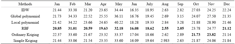
In order to prepare base monthly precipitation and temperature patterns, different geostatistical methods are compared to each other using cross validation technique.

Tables 4 and 5, show RMSE (Root Mean Square Error)

values of the six interpolation methods for precipitation and temperature data, respectively. Results show that RBF and IDW methods can be utilized for preparation of

0 10 20 30 40 50 60

0 100 200 300 400 500 600 700

Q(

m

3/s

)

Time(days) Observed

Predicted

Figure 5. Simulated and observed hydrographs for validation period during 2003-2004.

Figure 6. Mean of temperature in Ardabil station for the base (1961-1990) and future (2070-2100) period.

precipitation and temperature patterns. Therefore, pre- cipitation and temperature patterns are prepared for all months using these methods. Future monthly precipita- tion and temperature patterns are retrieved using the ex- plained method in Section 3.1.3. The samples of precipi- tation and temperature patterns in January of 2100 are shown in Figures 8 and 9.

4.3. Future Discharge Results

After calibration and validation of HSPF model to the

Figure 7. Mean of precipitation in Ardabil station for the base (1961-1990) and future (2070-2100) period.

watershed, PRECIS model base and future data series is used as the input to HSPF model. Table 6 shows the dif-

Table 4. RMSE values of the six interpolation methods for precipitation data.

Methods Jan Feb Mar Apr May Jun July Aug Sep Oct Nov Dec

IDW 21.44 33.38 21.20 23.65 34.44 16.35 18.95 2.63 2.82 27.03 24.25 22.24

Global polynomial 21.73 34.33 22.52 25.55 36.11 16.76 19.45 2.69 3.15 24.07 27.50 21.35 Local polynomial 21.42 34.22 23.66 24.65 40.22 18.28 19.33 2.84 3.28 21.88 28.90 21.46 RBF 20.85 31.01 20.59 19.63 32.18 16.08 18.62 2.55 2.05 23.78 24.77 21.12 Ordinary Kriging 22.37 33.60 21.67 23.32 33.37 17.04 18.66 2.62 2.89 21.73 23.82 21.14 Simple Kriging 21.44 33.06 21.54 23.35 33.60 16.09 19.64 2.983 2.63 21.87 24.06 21.84

Table 5. RMSE values of the six interpolation methods for temperature data.

Method Jan Feb Mar Apr May Jun July Aug Sep Oct Nov Dec

IDW 4.88 2.81 4.22 2.34 2.56 3.39 3.49 4.72 4.37 6.13 6.33 3.95 Global polynomial 6.16 3.64 5.91 2.36 3.35 4.18 4.50 5.82 5.56 7.97 9.04 5.54

Local polynomial 6.45 3.88 6.26 2.34 3.16 4.30 4.59 5.96 5.72 8.16 9.45 5.88

RBF 5.15 2.78 4.13 2.24 2.42 3.51 3.62 4.99 4.63 5.96 6.07 4.08

Ordinary Kriging 4.96 2.62 3.78 2.20 2.32 3.50 3.76 4.81 4.99 6.45 6.55 4.23

Simple Kriging 5.07 2.93 3.86 2.45 2.38 3.64 3.82 4.92 4.86 6.21 6.30 3.38

Figure 8. Precipitation pattern on January of 2100.

Figure 9. Temperature pattern on January of 2100.

takes place on April (Table 6).

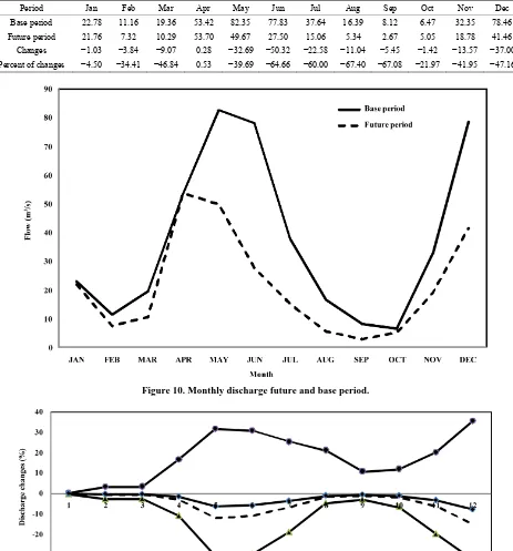
Figure 10 shows monthly discharge in the future and

base periods. This figure demonstrates that the peak dis- charge in the future period would happen one month ear- lier. It is because of increasing temperature and earlier beginning of snow melting. Generally, results show that in the future, the discharge of Gharehsoo River water- shed would decrease in the all of months. It might make problem for agriculture of studied region; because, Gharehsoo watershed is one of the most important re- gions for production of crops in Iran and plays an impor- tant role in economic growth and food of this country.

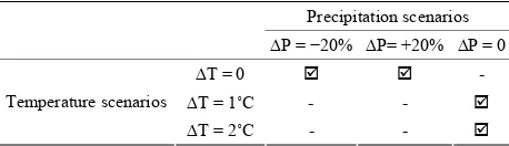
4.4. Sensitivity Analysis

In this section, the sensitivity of precipitation and tem- perature to runoff is investigated. Sensitivity analysis is performed in four hypothetical scenarios for future cli- mate (Table 7). In two hypothetical scenarios, the pre-

cipitation is increased and decreased 20 percent. In the other scenarios, the temperature is increased 1˚C and 2˚C. Results of sensitivity analysis are exhibited in Figure 11.

It is obvious that 1˚C and 2˚C increase of temperature lead to 0% - 8% and 0.1% - 15% decrease of average monthly discharge, respectively. In addition, Figure 11

exhibits that monthly discharge increases 0.3 - 35.6 per- cent due to 20% increase of precipitation. Similarly, monthly discharge decreases 0.3 - 32.6 percent due to 20% decrease of precipitation.

5. Conclusions

Table 6. Difference between monthly discharges in the base and future periods.

Period Jan Feb Mar Apr May Jun Jul Aug Sep Oct Nov Dec

Base period 22.78 11.16 19.36 53.42 82.35 77.83 37.64 16.39 8.12 6.47 32.35 78.46

Future period 21.76 7.32 10.29 53.70 49.67 27.50 15.06 5.34 2.67 5.05 18.78 41.46

Changes −1.03 −3.84 −9.07 0.28 −32.69 −50.32 −22.58 −11.04 −5.45 −1.42 −13.57 −37.00 Percent of changes −4.50 −34.41 −46.84 0.53 −39.69 −64.66 −60.00 −67.40 −67.08 −21.97 −41.95 −47.16

Figure 10. Monthly discharge future and base period.

Figure 11. Results of sensitivity analysis of mean monthly runoff to the precipitation and temperature in the Gharehsoo River watershed.

Gharehsoo River. In this study, the different geostatisti- cal methods were utilized for the estimation of present monthly patterns of precipitation and temperature. The cross validation technique was utilized for evaluation of

Table 7. Hypothetical scenarios of future climate.

Precipitation scenarios

∆P = 0

∆P= +20%

∆P = −20%

-

 

∆T = 0



- -

∆T = 1˚C



- -

∆T = 2˚C Temperature scenarios

duce climate data of base (1960-1990) and future (2070- 2100) periods based on B2 scenario with 50 × 50 km resolution. In addition, by combination of base and future precipitation and temperature data with the extracted precent patterns for precipitation and temperature, the future patterns for monthly precipitation and temperature were extracted. The comparison between base and future monthly precipitation and temperature showed that future precipitation is more than the base precipitation on Janu- ary, February, March, September and December and fu- ture temperature increases 2˚C - 4˚C in winter, 2˚C - 5˚C in spring, 3˚C - 5˚C in summer and 2˚C - 4˚C in autumn.

The base and future precipitation and temperature pat- terns were introduced to validated HSPF model for the simulation of monthly runoff in the base and future peri- ods. The results show that in the future, the discharge of Gharehsoo River watershed decreases in all of the months. In addition, the peak discharge in the future period hap- pens one month earlier, because of increase of tempera- ture and earlier beginning of snow melting season. Fi- nally, the sensitivity of precipitation and temperature to runoff was investigated and the results showed that 1˚C and 2˚C increase of temperature leads to 0% - 8% and 0.1% - 15% decrease of average monthly discharge, re- spectively. In addition, monthly discharge increases 0.3% - 35.6% and decreases 0.3% - 32.6% due to 20% increase and decrease of precipitation, respectively.

REFERENCES

[1] L. Nash and P. Gleick, “The Sensitivity of Streamflow in the Colorado Basin to Climatic Changes,” Journal of Hy- drology, Vol. 125, No. 3, 1991, pp. 221-241.

[2] R. L. Wilby, L. E. Hay and G. H. Leavesley, “A Com- parison of Downscaled and Raw GCM Output: Implica- tions for Climate Change Scenarios in the San Juan River Basin, Colorado,” Journal of Hydrology, Vol. 225, No. 1,

1999, pp. 67-91.

[3] W. Arnell, “Climate Change and Global Water Resources,”

Journal of Global Environmental Change, Vol. 9, No. 1,

1999, pp. 31-49.

[4] P. S. Yu, T. C. Yang and C. K. Wu, “Impact of Climate Change on Water Resources in Southern Taiwan,” Jour- nal of Hydrology, Vol. 260, No. 1, 2002, pp. 161-175. [5] T. G. Huntington, “Climate Warming Could Reduce

Run-off Significantly in New England, USA,” Journal of Ag- ricultural and Forest Meteorology, Vol. 117, No. 3-4, 2003, pp. 193-201.

[6] H. Chen, S. Guo, C. Y. Xu and V. P. Singh, “Historical Temporal Trends of Hydro-Climatic Variables and Run-off Response to Climate Variability and Their Relevance in Water Resource Management in the Hanjiang Basin,”

Journal of Hydrology, Vol. 344, No. 3-4, 2007, pp. 171-

[7] M. Akhtar, N. Ahmad and M. J. Booij, “The Impact of Climate Change on the Water Resources of Hindukush- Karakorum-Himalaya Region under Different Glacier Co- verage Scenarios,” Journal of Hydrology, Vol. 355, No. 1, 2008, pp. 148-163.

[8] S. Vicune, R. D. Garreaud and J. McPhee, “Climate Change Impacts on the Hydrology of a Snowmelt Driven Basin in Semiarid Chile,” Journal of Climatic Change, Vol. 105, No. 3, 2011, pp. 469-488.

[9] M. Zarghami, A. Abdi, I. Babaeian, Y. Hassanzadeh and R. Kanani, “Impacts of Climate Change on Runoffs in East Azerbaijan, Iran,” Journal of Global and Planetary Change, Vol. 78, No. 3-4, 2011, pp. 137-146.

[10] V. M. F. Jacomino and E. D. Fields, “A Critical Ap- proach to the Calibration of a Watershed Model,” Journal of American Water Resource Association, Vol. 33, No. 1, 1997, pp. 143-154.

[11] M. Albek, U. Ogutveren and E. Albek, “Hydrological Modeling of Seydi Suyu Watershed (Turkey) with HSPF,”

Journal of Hydrology, Vol. 285, No. 1, 2004, pp. 260-271.

[12] J. C. Imhoff, J. L. Kittle, M. R. Gray and T. E. Johnson, “Using the Climate Assessment Tool (CAT) in US EPA BASINS Integrated Modeling System to Assess Water- shed Vulnerability to Climate Change,” Journal of Water Science & Technology, Vol. 56, No. 8, 2007, pp. 49-56.

[13] N. Al-Abed and M. Al-Sharif, “Hydrological Modeling of Zarqa River Basin—Jordan Using the Hydrological Si- mulation Program—FORTRAN (HSPF) Model,” Water Resources Management, Vol. 22, No. 9, 2008, pp. 1203-

1220.

[14] F. Abdulla, T. Eshtawi and H. Assaf, “Assessment of the Impact of Potential Climate Change on the Water Balance of a Semi-Arid Watershed,” Water Resources Manage- ment, Vol. 23, No. 10, 2009, pp. 2051-2068.

[15] C. C. Gordon, R. Cooper, C. A. Senior, H. Banks, J. M. Gregory, T. C. Johns, J. F. B. Mitchell and R. A. Wood, “The Simulation of SST, Sea Ice Extents and Ocean Heat Transports in a Version of the Hadley Centre Coupled Model without Flux Adjustments,” Climate Dynamics,

Vol. 16, No. 2-3, 2000, pp. 147-168.

Wilson, G. J. Jenkins and J. F. B. Mitchell, “Generating High Resolution Climate Change Scenarios Using PRE- CIS,” Met Office Hadley Centre, Exeter, 2004.

[17] K. Johnston, J. M. VerHoef, K. Krivoruchko and N. Lu- cas, “Using ArcGIS Geostatistical Analyst,” ESRI Press, Redlands, 2001.

[18] H. H. Crawford and R. K. Linsley, “Simulation in Hy- drology: Stanford Watershed Model IV,” Technical Re- port No. 39, Stanford University, Stanford, 1966.

[19] A. S. Donigian and H. H. Davis, “User’s Manual for Ag- ricultural Runoff Management (ARM) Model,” USEPA, Athens, 1978.

[20] A. S. Donigian and N. H. Crawford, “Modelling Non- point Pollution from the Land Surface,” Environmental Research Laboratory, Athens, 1976.

[21] A. S. Donigian and W. C. Huber, “Modeling of Nonpoint Source Water Quality in Urban and Non-Urban Areas,” USEPA, Athens, 1991.

[22] A. S. Donigian, B. R. Bicknell and J. C. Imhoff, “Hydro- logical Simulation Program—FORTRAN (HSPF),” In: V. P. Singh, Ed., Computer Models of Watershed Hydrology,

Water Resources Pubs, Highlands Ranch, 1995, pp. 395- 442.

[23] Hydrocomp Inc., “Hydrocomp Water Quality Operations Manual,” Hydrocomp, Inc., Palo Alto, 1997.

[24] B. R. Bicknell, J. C. Imhoff, J. L. Kittle, T. H. Jobes and A. S. Donigian, “Hydrological Simulation Program For- tran: User’s Manual for Release 12.2. US EPA Ecosystem Research Division, Athens, GA and US,” 2005.

[25] E. S. Chung, K. Park and K. S. Lee, “The Relative Im- pacts of Climate Change and Urbanization on the Hydro- logical Response of a Korean Urban Watershed,” Journal of Hydrological Processes, Vol. 25, No. 4, 2011, pp. 544-

[26] B. R. Bicknell, J. C. Imhoff, J. L. Kittle, R. C. Johanson and A. S. Donigian, “Hydrological Simulation Program- Fortran User’s Manual for Release 10,” Environmental Research Laboratory Office of Research and Develop- ment US Environmental Protection Agency, Athens, 1993. [27] A. S. Donigian, B. R. Bicknell, J. C. Imhoff and J. L.

Kittle, “Application Guide for Hydrological Simulation Program-Fortran (HSPF),” Prepared for US EPA, EPA- 600/3-84-065, Environmental Research Laboratory, Ath- ens, GA, 1984.

[28] EPA, “BASINS Technical Note 6,” Estimating Hydrol- ogy and Hydraulic Parameters for HSPF, 2001.