Munich Personal RePEc Archive
Mean-Reverting Stochastic Processes,
Evaluation of Forward Prices and
Interest Rates
Makhankov, V. G. and Aguero-Granados, M. A.
Universidad Autonoma del Estado de Mexico, Toluca, Mexico, Bussiness Math, Santa Fe, NM USA, Los Alamos National Laboratory
15 November 2009
Mean-Reverting Stochastic Processes,
Evaluation of Forward Prices
and Interest Rates
Vladimir G. Makhankov
1, Maximo A. Aguero-Granados
21)
BusinessMath, Santa Fe NM, USA
2)
Facultad de Ciencias, Universidad Autonoma del Estado de Mexico, Instituto Literario 100, Toluca 50000, Mexico
.
Key words: Stochastic Differential Geometry, Mean-Reverting Stochastic Processes and Term Structure of Specific (Some) Economic/Finance Instruments.
Address correspondence to V. Makhankov: 4148 Chaparron Pl. Santa Fe, NM 87507 USA, E-mail: [email protected]
2)
2 ABSTRACT
We consider mean-reverting stochastic processes and build self-consistent models for forward price dynamics and some applications in power industries. These models are built using the ideas and equations of stochastic differential geometry in order to close the system of equations for the forward prices and their volatility. Some analytical solutions are presented in the one factor case and for specific regular forward price/interest rates volatility. Those models will also play a role of initial conditions for a stochastic process describing forward price and interest rates volatility.
Subsequently, the curved manifold of the internal space i.e. a discrete version of the bond term space (the space of bond maturing) is constructed. The dynamics of the point of this internal space that correspond to a portfolio of different bonds is studied. The analysis of the discount bond forward rate dynamics, for which we employed the Stratonovich approach, permitted us to calculate analytically the regular and the stochastic volatilities. We compare our results with those known from the literature.
I. INTRODUCTION
In this paper we give a self-consistent framework for describing and analyzing (evaluating) two different economic instruments that play a fundamental role in evaluating corresponding derivatives and hence in the risk management. Both have the term structure (mature at a definite time) and the first, discount bond interest rates, is going at finance market, the second, forward prices, at the commodity one. On the basis of stochastic differential geometry (DSG) equations that describe spot price/interest rate dynamics and long term dynamics (entire forward prices/interest rates curves) we construct mathematical models which turn out to be very similar.
1998, Clewlow and Strickland 1999 to mention a few. Later we give more detailed references in due places.
The paper is organized as follows: In section II we give a very short introduction to the stochastic differential geometry, i.e. Brownian motion on curved manifolds (e.g., sphere), Makhankov 1995 and 1997, that allows us to take into account stochastic behavior of the forward prices/interest rates volatility and to close the system of equations. Section III presents the study of forward price dynamics and possible solutions for the forward price curve, its mean and volatility. Section IV is devoted to study of interest rates dynamics and some solutions. Finally, section V contains our conclusions.
II.
STOCHASTIC DIFFERENTIAL GEOMETRYRecent development in physics shows that all types of interactions admit geometrization. In the most transparent form it can be seen in the theory of the so-called (1+1) dimensional integrable systems, where in a consistent manner the relationship is established between geometry of the internal (isotopic) space and the type of interaction, see, e.g. Makhankov and Pashaev 1992.
In general discrete form the stochastic equation governing forward prices/rates dynamics (instruments with an internal space) is as follows:
1
( ) ( ) ( ) ( )
n
i i i
p p
dX t f t
σ
t dW t=
= +
∑
(II-1)where i( )
f t is the price/rate drift, i( )
p t
σ is the price/rate volatility and the index i spans the internal space (details will be discussed later on).
From the other hand the equations of stochastic differential geometry that describe the Brownian motion (diffusion) on a curved space (manifold) in terms of Stratonovich differentials (see Stratonovich 1968) read, Kendal 1987, Makhankov 1997:
1
, 1
( )
( )
n
i i q
q q m
i i j k
q jk q
j k
dX
t
dW
t
d
dX
=
=
=
Σ
Σ = −
Γ Σ
∑
∑
(II-2)
Where
X
i is an m-dim. vector (a point in an m-dim curved space), i q4
a natural frame on a patch of the bundle and i jk
Γ are conexion coefficients (Christoffel’s symbols) through which a curvature of the space is given. The first equation describes an elementary shock a Brownian particle undergoes due to a collision with the stochastic background.
If we assume the state space to be a Riemannian manifold, then the inverse of the Riemannian metric is given by
ij qi qj q
g =
∑
σ σ (II-3) such thatg gij jk =δik Here we face two cases:
1) the conexion is compatible with the metric,
2) the conexion is “arbitrary”, and can be determined, e.g. by matching some Ito process governing the system.
In the first case the conexion is expressed in terms of the Riemannian Γ metric gij, Dubrovin et al, 1984 and we come to a closed system of stochastic differential equations describing a stochastic path on a Riemannian manifold.
In the second case
1
( )
2
i i i i i q
q q q
q
dX = dσ +σ ≡ f dt +
∑
σ dW, in order to close our system of equations we match the drift term of the Ito process for the forward price/interest rates (II-1) with the drift term in SDG eqns. (II-2). Then the SDG equations will describe the forward price/interest rates dynamics as a Brownian motion in a curved space with the curvature defined by their drift. Rewriting eq. (II-2) in Ito representation one obtains
(II-4)
with the drift term due to the second eq. (II-2) being
, , ,
1 1
2 2
i k i j i k j
q k j q k j
j k q k j
f = −
∑
σ Γ σ = −∑
Γ g (II-5)In order to use SDG equations (II-2), equations (II-4) and (II-1) have to be identical, i.e. i i, i i
q q
f = f σ =σ whence
,
1 ( )
2
i i k j
k j k j
f t = −
∑
Γ g (II-5a)i 2 i( )
k j g f tk j m
Γ − (II-6)
This gives us the relationship between the conexion Γ, the drift i( )
f t of the
forward price/interest rate and the volatility structure i q
σ through the space metric i j
g .
If the drift only depends on the geometrical part
i( ) ( i)
q
f t = f σ
the system of stochastic differential equations (II-2) becomes closed and self-consistent.
It is well known from differential geometry that one of the most important characteristics of a manifold is its conexion curvature tensor
−Rijkl = ∂ Γ − ∂ Γ + Γ Γ − Γ Γk ijl l ijk ipk jlp ipl pjk
Namely this tensor defines invariant geometrical properties of a manifold and vanishes in the Euclidean case: Rijkl =0. A nonzero conexion yet does not imply a curved space (it could be related to fictitious-inertial forces) and a nonzero curvature tensor surely does, implying essential drift presence in the system studied. Sometimes instead of the curvature tensor i
jkl
R it is easier to
calculate the so-called scalar curvature
, ,
il i jil i j l
R=
∑
g Rthat gives us a clear understanding of the state space nature as well. More comprehensive review on these issues is given in Annex 1.
III.
FORWARD PRICES AND THEIR MODELINGDefinition1. A forward contract is a particularly simple derivative and is an agreement to buy (a long position) or to sell (a short one) an asset at a certain future time (maturity date T) for a certain price (the delivery price
K).
At time the contract is initiated the delivery price should be such that the contract value for both parties is zero. The contract is obligatory.
6
The forward price and the delivery price are equal at the time the contract is entered into. As time passes, they go apart since pre-specified initially delivery price is constant. Therefore we can think of the forward price as the delivery price at current time t.
There is a very well-known formula relating the forward price and the spot price, Hull 1993
F t T
( , )
=
S t e
( )
(r u y T t+ − )( − )(III-1)
where r is a risk-less interest rate, u is a storage rate and y a convenience yield. Both the storage rate and especially the convenience yield are usually unknown functions and the convenience yield can be a stochastic process.
Following Cortazar & Schwartz 1994, we will describe the dynamics of the forward price by the equation
1 ( , )
( , ) ( )
n
p p
p
dF t T
t T dW t
F =
=
∑
Σ (III-2)where Σp( , )t T is the volatility corresponding to a p-th random factor described
by the Wiener generator p( )
dW t . So model (III-2) describes the n-factor
dynamics of the forward curve F
(
t,T
).
We assume that interest rates are deterministic and future prices are equal to forward prices (see, e.g. Hull 1993). In (III-2) we have n independent sources of uncertainty
2
0 0
1
1
( , ) (0, ) ex p ( , ) ( , ) ( ) 2
n t t
i
i i
i
F t T F T τ T dτ τ T dW τ
=
= − Σ + Σ
∑
∫
∫
that drive the evolution of the forward curve F(t,T). By integrating (III-2) we have (using Ito’s lemma)
(III-3)
Then for the spot price by definition, S(t) = F(t,t), and we have by setting T = t
2
0 0
1
1
( ) (0, ) ex p ( , ) ( , ) ( ) 2
n t t
i
i i
i
S t F t τ t dτ τ t dW τ
=
= − Σ + Σ
∑
∫
∫
(III-4)By differentiating (III-4) over t we have got the stochastic differential equation for the spot price
1 0 0
1
( , ) ( , )
( ) ln (0, )
( , ) ( ) ( ) ( , ) ( ) t t n i i i i i n i i i t t
dS t F t
t d dW dt
S t t t t
t t dW t
τ τ
τ τ τ
=
=
∂ ∂Σ ∂Σ
= − Σ −
∂ ∂ ∂ + Σ
∑ ∫
∫
∑
(III-5)The term in the curled parentheses can be interpreted as an equivalent to the sum of the deterministic risk-less rate of interest r
(
t
)
and a convenience yieldy
(
t
)
which in general should be stochastic. Many well-known models are special cases of this general approach.Now it’s well known that the volatilities in (III-2) are stochastic processes themselves. What kind of stochastic processes they could be? To answer this question we resort to the stochastic differential geometry, Makhankov 1995, 1997 described above. As a result, we obtain a self-consistent model described by the system of stochastic equations. To solve them we have to specify initial conditions:F(0, ), (0)T S and Σi(0, )T .
Ergo, the dynamics of the forward price logarithm is given by the equation
2
1 1
1
ln ( ( , )) ( , ) ( , ) ( )
2
n n
q
q q
q q
d F t T t T d t t T d W t
= =
= −
∑
Σ +∑
Σ (III-6)in
Ito differentials. If we assume the internal term space of the model being
discrete (what is true in reality) we have gotF t T( , ) = F t kT( , ) =F tk( ) Now denoting
k
( ) ln
k( )
X
t
=
F t
(III-7) we come to the equation2
1 1
1
( )
( )
( ),
(1,..., )
2
n n
i i i q
q q
q q
dX t
t dt
dW
t
i
m
= =
= −
∑
Σ
+
∑
Σ
∈
(III-8)written in Ito differentials.
2 2
1 0 1 0
1
ln (( )) {ln ( (0, )) ( , ) }, ( , ) } 2
T T
n n
i i
i i
S T N F T τ T dτ τ T dτ
= =
≈ − Σ Σ
8
If we wish that the dynamical model of forward price should correspond to the pure Brownian motion in the curved manifold we have to equate eq. (III-7) to the first equation of system (II-1) also written in the Ito differentials
1 , , 1
1
1
( )
(
)
( )
( )
2
2
n n
i i i q i k j i q
q q jk q q q
q j k q q
dX t
d
dW
t
dt
dW
t
= =
=
∑
Σ + Σ
= −
∑
Γ Σ Σ
+
∑
Σ
(III-9) Then we have the equation for self-consistency of the model
2
1 ,
( )
n n m
i i k j
q jk q q
q q j k
t dt dt
=
Σ = Γ Σ Σ
∑
∑∑
(III-10)Resolving this equation with respect to
,
i i j
k q j k q
A
= Γ Σ
we obtain
,
i i i
k q q k
A
= Σ
δ
Substituting this equation into the second one of (II-1) we come to the equation
1
( )
( )
n
i i i q
p p q
q
d
t
dW
t
=
Σ
= −Σ
∑
Σ
(III-11)
Now our system is closed and self-consistent since the curvature of the term space is defined by the “force term” (the trend) in the equation for the price dynamics.
So we have to solve the following system of equations
1 1
( ) ( )
( ) ( )
n
i i q
q q
n
i i i q
p p q
k
dX t dW t
d t dW t
=
=
= Σ
Σ = −Σ Σ
∑
∑
2
1 1
2
1
( ) ( ) ( )
2
= ( )
n n
i i i q
q q
q q
n n
i i i i i p
q q p q p
p p
dX t t dt dW t
d dt dW
= =
= − Σ + Σ
Σ Σ Σ − Σ Σ
∑
∑
∑
∑
(III-12)
From the first equation of (III-12) we infer that
X has a Gaussian distribution.
What about the volatility?III.1 ONE - FACTOR REDUCTIONS OF THE MODEL.
Let us consider a one-factor reduction of the model. It makes sense since as is well-known some, may be even many power markets as well as financial ones show almost one-factor behavior: principal component analysis gives from 80% to even 90% of the total contribution to the main component according to Clewlow & Strickland (1999), Wilmott (2001).
So, one factor:
dW
p=
dW
andΣ =
iY
then
dY
=
Y dt Y dW
3−
2(III-13)
and the Fokker-Planck (FP) equation for the transition probability ρ reads
(
31
4)
2
t
ρ
yy
yy
ρ
∂ = ∂ − + ∂
(III-14)Let us consider stationary solutions of (III-14). Then we have
3 1 4
( ) =0
2
y y yy ρ
∂ − + ∂
with a solution
cy 3a
y
ρ
= + (III-15)Let us consider the related Stratonovich process
n
i i i p
q q p
p
d
Σ = − Σ
∑
Σ
dW
or for a single-factor, single-term process i
Z = Σ we have
dZ
= −
Z dW
2(III-16)
10
2 2 1
( )
2
t
ρ
z z zzρ
∂ = ∂ ∂
and stationary solutions
a3
z
ρ
= (III-17)Then we see that both processes have similar distributions if y is sufficiently small
a y
c
<<
It was the Stratonovich process. For the Ito process we have eq. (III-8). The mean can be estimated from the trend term by the following reasoning: taking average of the equation we have for Σ =< Σ > +s and < >=s 0
3 3
3
2 3d
s
s
< Σ >=< Σ >=< + < Σ >> = <
>< Σ > + < Σ >
Where the variance
<
s
2> ≈ < Σ >
t
4and the first term in the equation can be neglected. Now since < Σ > = < Σ − Σ > = < Σ >d t+1 t d we come tod < Σ > = < Σ >3 dt
with the solution
2
2
1 2
1
(1+ )
1 t t
σ σ σ
σ
< Σ > = ≈
−
Armed with the above knowledge we can calculate the forward price curve. In order to obtain analytical estimate we restrict ourselves to “short time” horizons:
2
1 t
σ << (III-18)
and consider only first two initial terms in the asymptotic expansion.
Earlier, we consider the statistical properties of the model and its short time horizons. In what follows we study the dynamics of the model in more detail.
Let us consider the single factor version of model (III-2). Then for F(t,T) we have
( , ) ( , ) ( ) and ( , ) ( ) ( , )
dF t T
t T dW t F t t S t
F t T = Σ = (III-19)
or using Ito’s lemma
2
1
ln ( , ) ( , ) ( , ) ( )
2
Integrating once we obtain
or
2
0 0
1
( , ) (0, ) ex p { ( , ) ( , ) ( )} 2
t t
F t T = F T −
∫
Σ u T du+ Σ∫
u T dW u (III-20)This solution is defined so far accurate to an arbitrary function F(0,T). To restrict this freedom we can specify a random process for the spot price S(t). Now since S(t)= F(t,t), knowing the equation for S(t) gives us the equation for F(0,T) through the parameters involved in the equation for S(t).
Let us consider a mean-reverting process for S(t), viz.
dS ( ln )S dt ( )t dW t( )
S =
α µ
− +σ
(III-21)This kind of processes is very popular in econometrics since, for example, forward prices as well as interest rates appear over time to be pulled back to some long average level. This phenomenon is known as mean reversion, see Hull 1993, p388. Also Schwartz’s 1997 model for the commodity price dynamics used a single factor mean-reverting process. In fact, equation of type (III-21) appeared in physics long ago and was assumed to describe the so-called Ornstein-Uhlenbeck process, see appendix for more detail.
From the other hand, eqn. (III-20) gives
2
0 0
1
( ) (0, ) ex p { ( , ) ( , ) ( )}
2
t t
S t = F t −
∫
Σ u t du + Σ∫
u t dW u (III-22)
i.e. lnS is normally distributed with
the mean = 2
0
1
ln ( , ) 2
t
F −
∫
Σ u T duthe dispersion = Σ( , )t t
Also from eqn. (III-22) taking the log we have
2
0 0
1
ln ( ) ln (0, ) ( , ) ( , ) ( )
2
t t
S t = F t −
∫
Σ u t du+ Σ∫
u t dW u (III-23)
Then by differentiating over t one has 2
0 0
( , )
1
ln
( , )
( , )
( )
(0, )
2
t t
F t T
u T du
u T dW u
12
Easy to check out that from Ito’s lemma follows that
2
1
ln ( )
( , )
2
dS
d
S t
t t dt
S
+ Σ
=
Therefore
0 0
( ) ln (0, )
[ ( , ) ( , ) ( , ) ( )]
( )
( , ) ( )
t t
t t
dS t F t
u t u t du u t dW u dt
S t t
t t dW t
∂
= − Σ Σ + Σ
∂ +Σ
∫
∫
(III-24)
Now if the spot process underlying the forward price dynamics is defined by eqn. (III-21) we have the self-consistent system of equations:
σ
( )
t
= Σ
( , )
t t
(III-25a)0 0
ln (0, )
( ln ) t ( , ) ( , )t t t( , ) ( )
F t
S u t u t d u u t d W u
t
α µ
− = ∂ − Σ Σ + Σ∂
∫
∫
(III-25b)
Rewrite eqn. (III-23) in the form
2
0 0
1
( , )
( ) {ln ( ) ln (0, )}
( , )
2
t t
u t dW u
S t
F
t
u t du
Σ
=
−
+
Σ
∫
∫
(III-26)
We can easily solve the system of equations (III-24), (III-25) and (III-26) if
1) The first group of models
∂ Σ
t 1( , )
u t
= − Σ
α
1( , )
u t
(III-27)Or in more general case
2) The second group of models
∂ Σ
t 2( , )
u t
= − Σ
α
2( , )
u t
+
f t
( )
(III-28)
2
0
0
ln (0, )
1
ln ( ) [
( , )
( , ) ( , )
2
( , )
( )]
( , )
( )
t
t t
t
F
t
d
S t
t t
u t
u t d u
t
u t dW u dt
t t dW t
∂
=
− Σ
− Σ
Σ
∂
+ Σ
+ Σ
where f(t) is a known function of t. Those conditions allow canceling stochastic integrals in the equations (akin to the risk-less condition) and are necessary for solvability of the whole problem. They look very plausible for they mean that the volatility of the forward price decays from one level to another or zero.
For the first group of models if we substitute eqn (III-27) into (III-25) and use (III-26) we come to
2 1
1 0 1 1
ln (0, ) 1
ln (0, ) ( , ) ( )
2 t
F t
F t u t du t
t α α µ
∂ + = − Σ ≡ Φ
∂
∫
(III-29)In general case (III-28) we have
2
2 0 2 0 2 0
1
( ) ( , ) ( , ) ( ) ( ) ( )
2
t t t
t α µ u t du u t f u du f u dW u
Φ = − Σ + Σ −
∫
∫
∫
(III-30)Equation (III-29) along with (III-30) can be readily solved, providedwe know the forward price volatility Σ( , ).t T
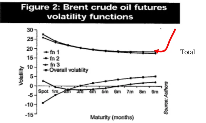
Below we give the graphs of modeled volatility curves and real ones.
2 4 6 8 10
0.1 0.2 0.3 0.4
14
2 4 6 8 10
[image:15.612.139.483.384.589.2]0.1 0.2 0.3 0.4 0.5
Fig 1. Zero maturity asymptotic of the. Fig. 2. Nonzero maturity asymptotic.
In reality we have the situation very close to the second curve, see Clewlow & Strickland 1999.
(0, ) S T = 0.2Exp(-0.5 ) 0.1T +
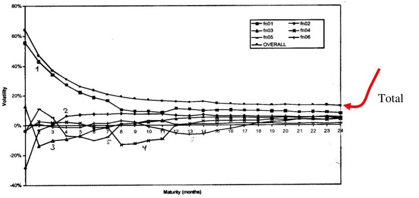
Fig. 4. Principal component analysis for Natural gas.
The solution of (III-29) (obtained by the variation of constant method) is
0
ln (0, )
t{
t u( )
}
i i
F
t
=
e
−α∫
e
αΦ
u du
+
const
Since at t = 0 lnFi(0, 0) ln (0)= Si then
0
ln
(0, )
t{
t u( )
ln (0)}
i i i
F
t
=
e
−α∫
e
αΦ
u du
+
S
(III-31) We see µ not necessarily be a constant. It can be a function of time.For example: if the forward price process volatility
1) is a regular function of time, e.g. a first class three-parameter exponential model
1( , ) 1 ( )
T t
t T
σ
e−α −Σ = (III-32a)
and
2) ( ) 1
t
t eκ
µ =µ (a constant κ can be both negative or positive)
Total
[image:16.612.130.543.139.335.2]16
Then the integral is exactly evaluated as
2
2
1 1
1(0, ) exp{ ln (0)1 ( ) (1 ) }
4
T T T T
F T e α S αµ eκ e α σ e α
α κ α
− − −
= + − − −
+ (III-33)
Now by setting κ =0 we come to the well-known result, Clewlow and Strickland 1997:
2
2 1
1 (0, ) exp ln 1(0) 1(1 ) (1 )
4
T T T
R
F T e α S µ e α σ e α
α
− − −
= + − − −
(III-34)
It’s easily seen that in this case the forward price curve is regular with zero volatility.
A bit more tedious calculations are needed to get the forward price curve for the second class four-parameter model:
2( , ) 1 ( ) 0
T t
t T
σ
e−α −σ
Σ = + (III-32b)
In this case we have got
2 2 2
2 2 1 0
1
ln (0, ) (0) (1 ) (1 ) 2 ( 1 )
4
T T T T
R
F T e α S µ e α σ e α σ αT e α
α
− − − −
< >= + − − − − − +
(III-35)
and
[
]
02 2 2 2 2 22
ln (0, ) 2 (1 ) (2 )
2
T T
R
Var F T
σ
e αα
Tα
T e αα
Tα
− −
= − + − + (III-36)
I.e. in the second case, even for regular volatility of the forward price process
( , )t T
Σ the forward price curve itself F2R( , )t T becomes stochastic with nonzero
volatility (III-36).
Even more tedious calculations needed to take into account the stochasticity of the forward price process volatility Σ( , )t T . For that we should solve the second equation of the stochastic differential geometry (III-12). This equation is self-consistent and can be separately analyzed.
Under the same assumption (single-factor model) for Stratonovich process it reads,
1 ( , ) ( 1 ) ( , )2 ( )
str str
St St
dΣ t T = − Σ t T d W t (III-37)
3 2
1
(
1)
(
1)
i i i
St St St
d
Σ = Σ
dt
− Σ
dW
(III-38)for the Ito process.
From eqns. (III-15) and (III-17) one can see that the solutions to both FP equations are identical if c<<a or, e.g. when c = a. It means that in our case the Stratonovich process distributions are a subclass of the more general Ito’s distributions.
Since for Stratonovich processes we have the conventional calculus, we get
1
(0, ) ( , )
1 (0, ) ( )
str St t t t W
σ
τ
σ
τ
Σ = + or 1(0, )
( , )
1
(0, ) ( )
str St
T
t T
T W t
σ
σ
Σ
=
+
(III-39)and
1 2
(0, )
( , )
(1
(0, ) ( ))
str t t St
t
t
t W
σ
τ
σ
τ
∂ Σ
=
+
In eq. (III-39) W(t) is a standard Wiener process with mean-less and unity-variance Gaussian distribution. So we can express W(t) as a function of Σi
( ) 1 1 ( ) (0)
str str
W t
t
= −
Σ Σ (III-40)
Also it is easy to calculate the mean and variance of i( , )
t T
Σ for small t (short horizons)
2
4 2
[ ( , )] (0, ){1 (0, ) }
[ ( , )] (0, ) {1 6 (0, ) }
i i i
i i i
E t T T t T
Va t Tr t T t T
σ σ
σ σ
Σ ≈ +
Σ ≈ +
18
Now for the Stratonovich process we can go even further. Due to (III-40) we calculate the distribution for str( , )
t T
Σ by means of the formula
( )
(1/
str)
str(
str)
strstr
dw
w dW
d
d
d
ρ
=
ρ
Σ
Σ ≡
ρ
Σ
Σ
Σ
And for ( )
ρ
w is a Gaussian distribution we have
2 0
2
(1/ 1/ )
1
( ) exp
2 ( )
2
str str str
str str d t t
ρ
π
Σ − Σ Σ
Σ = − Σ
a distribution for a reciprocal of W(t).
Let us now continue discussing the dynamic properties of the forward curves.
In the first case, i.e. (0, ) 1
t
t e α
σ =σ − , we have
1 2 1
( , ) (0, )
( , )
(1 (0, ) ( )) (1 (0, ) ( ))
str str St t St t t t
t W t W
α
τ
σ
τ
α
σ
τ
σ
τ
Σ
∂ Σ = − = −
+ + (III-41)
Assume also that
σ(0, ) ( )T W T <<1 (III-42)
The last condition is very essential for the evaluations. This is because
( )
1 1 1 1
(0, ) ( ) T ( ) t T t ( ) T t t ( ) t
T W t e α W t e αW t e α e α W t e α t
σ =σ − ⇒≤ σ − − − ≤σ − ≈σ −
Here are two cases:
1) αT <<1 then σ12T <<1 and
2) αT >>1 σ12T is arbitrary
Now we have
1 1 2 1 1
( , ) ( )
( ) ( ) (0, )[1 2 (0, ) ( )]
t St St u t f u
f u W u t t W u
α
α
σ
σ
∂ Σ = − Σ +
= − (III-43)
And
3 2 2 4 2
1
0 0
1 1 9
( ) 2 (0, ) ( ) (0, ) ( ) (0, ) ( )
2 2
u u
u µ σ u W τ τd σ u W u σ u W u d u
Finally, we can solve eqns. (III-29) and (III-44) together to obtain ln (0, )F T as a stochastic process with the mean and volatility
2 1 1 4 2 3 1 2 1
ln (0, ) (1 ) ln (0) [1 (1 ) ] 2
1
[1 (1 3 (3 ) ) ]
6 2
{
}
T T T
St
T
F T e e S T e
T T e
α α α
α
µ σ α
α
σ α α
α
− − −
−
< >= − + − − +
− − + + (III-45)
and
{
}
2 6 2 2 ( )
1 1 0 0 0 0
6
4 2 2 2 2 2
1 2
[ln (0, )] 4 ( ) ( )
3 2 (3 6 4 )
12
T T u z
T u z
St
T T
Var F T e e du dz W d W t dt
Te T e T T
α α
α α
α σ τ τ
σ α α α
α
− − +
− −
= < >
= − + + + +
∫
∫ ∫
∫
(III-46)
In what follows we will compare our result with the conventional case
const
µ = and ( )
1 ( , ) 1
T t
R t T e
α
σ − −
Σ = with 2 2 2 1 1 1
ln (0, ) (1 ) ln (0) (1 ) 4
T T T
R
F T µ e α e α S σ e α
α
− − −
= − + − −
for specific values of the parameters involved.
By looking at (II-22) and (II-24) we see that the means differ by the terms proportional to some power ofσ1.
Underline again that the volatility of the spot price process S(t) is defined as
( )t ( , )t t
σ = Σ therefore
1
1 1 1 1
1
( ) [1 ( )]
1 ( )
t
t t t
t
e
t e e W t e
e W t
α
α α α
α
σ
σ
σ
σ
σ
σ
−
− − −
−
= ≈ − ≈
+ (III-47)
Then for the second class four-parameter model:
2 (0, ) ( 2 (0, ) 0), i.e. (0, ) 1 0
t
t St t St t t e
α
σ σ
α σ = − σ
∂ Σ = − Σ + + (III-48)
and
2 0 0
at
( ) , 1
1 ( )
t T W t σ σ α σ ≈ >> +
20
f u1( )=αW u( )σ2(0, )[1 2 (0, ) ( )]t − σ t W u
we have
2 0 0 0
3
( ) (0, ) ( )[ (0, ) 2 2 (0, )( (0, ) ) ( )] 2
f u =ασ +ασ t W u σ t − σ − σ t σ t − σ W u
and
2 2
2 0 0 0
0
(0, )
( ) {( 2 ) 2 (2 3 ) ( ) 3 (3 4 ) ( )}
2
t t
t α µ ασ σ σ σ σ σ W u σ σ σ W u du
Φ = −
∫
− − − + −Then up to the lowest orders terms with respect to W t( ) we obtain
2 2
2 2 1 0
2 2 2
1 0
1
ln[ (0, )] ln (0) (1 ) {( )
2 [ (1 ) (1 )]}
T T T
St
T
F T e S e e
T e T
α α α
α
µ σ σ
α
σ α σ α
− − −
−
< >= + − + −
− + − − (III-49)
and
2 2 0 2
[ln (0, )] { (4 1) (2 3)}
2
T T
St
Var F T σ e α e α αT
α
− −
= − + − (III-50)
The term structures of all these models, viz. F1R,F1St,F2R and F2St for specific
values of parameters: α µ σ σ, , 0, 1 and various S(0) are given at Figs. 5 – 8.
2 4 6 8 10
1.05 1.1 1.15 1.2 1.25
1.3 (0, )
i
F T
Fig. 5. Plots of Fi(0, )T as functions of the maturity T. The lowest (red) stands
for F1R, the next from it up (green) stands for F1St, one more up (blue) for F2R,
and the uppers (magenta) for F2St, whereas S(0) = 1.
2 4 6 8 10
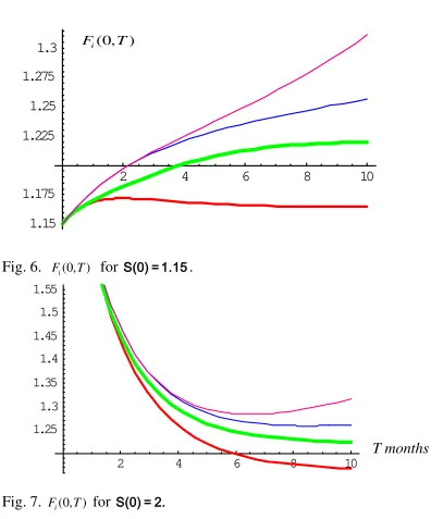
[image:22.612.88.495.142.619.2]1.15 1.175 1.225 1.25 1.275 1.3
Fig. 6. Fi(0, )T for S(0) = 1.15.
2 4 6 8 10
1.25 1.3 1.35 1.4 1.45 1.5 1.55
Fig. 7. Fi(0, )T for S(0) = 2.
In all calculations we put α =0.5, µ =0.2, σ1=0.14, σ0 =0.17. what is very
close to the values at the NYMEX Crude Oil market.
We see that for the short terms (around during two months) and out of the vicinity of S(0) 1.15= all four curves look very close to each other and then they
start do disperse about 7-10 % at the end of a year. The vicinity of the point
(0, )
i
F T
22
(0) 1.15
S = is the specific one. The function F1R( )T has a humped shape there, and
quite essentially differs from the other three curves that have no humps.
For the first exponential model the variances for both regular and stochastic variants are negligible. For the second model plots of the stochastic variance (yellow or the top curve), the “regular” one (red or the middle curve) and the difference between them (magenta, the bottom curve) are as follows.
2 4 6 8 10
0.025 0.05 0.075 0.1 0.125
0.15 0.175
Fig. 8.Variances for the second stochastic and regular models and their difference.
IV.
DISCOUNT BOND INTEREST RATES DYNAMICS.
Definitions. P(t,T) is the zero coupon (discount) bond price at time t with principle P(T,T)= $1, maturing at t = T.
r(t) is the short term interest rate.
( , ) p t T
ν is the volatility of P(t,T) corresponding to the p-th component of a n-dimensional vector Wiener process: 1
{ ,..., n}.
dW = dW dW
R(t,T) is the rate of in interest:
R t T( , ) ln ( , )P t T , 0 t T
T t
= − < ≤
− (IV-1)
such that
( , )( )
( , ) R t T T t
P t T =e− − (IV-2)
and R(t0 ,T) is a yield curve.
F(t,T) is the instantaneous forward rates (t≤T)defined bythe equation
[ln i(0, )]
Var F T
F t T( , ) ln ( , )P t T , 0 t T T
∂
= − < ≤
∂ (IV-3)
and finally
F t T( , ) R t T( , ) (T t) R t T( , )
T
∂
= + −
∂ (IV-4)
with the boundary condition at t = T :
F t t( , )= R t t( , )=r t( ) (IV-5)
Due to the weak market efficiency, P(t,T) along with the other variables are supposed to follow certain Markov processes. The most general of them is
1
( , ) ( , )[ ( , ) ( , ) ], 1,. . . ,
n
p p
p
d Pt T P t T µ t T d t ν t T d W p n
=
= +
∑
= (IV-6)This process is determined by (n+1) unknown functions µ( , )t T and νp( , )t T . In
the arbitrage-free case, Hull 1993 this equation rewritten for F(t,T) was shown to be reduced to a simpler equation only containing the unknown functions
( , ) p t T
ν :
1
( , ) { ( , ) ( , ) ( , ) p}
p p p
p
d Ft T σ t T ν t T d t σ t T d W
=
=
∑
− + (IV-7)where
( , ) p( , ) p
t T t T
T
ν
σ = −∂
∂ (IV-8)
The internal space or the system state space is a discrete version of the bond term space (the space of bond maturing). This space is an N-dimensional vector space with the metric E A t B t[ ( ) ( )] and is created by the vectors
X t( ) {= X t1( ),...,XN( )} { ( , ),..., ( ,t ≡ F t T1 F t TN)}
A point X t( ) {= X t1( ),...,XN( )}t
in this space corresponds to a portfolio (a set) of different bonds, and portfolio dynamics is a movement of the corresponding point in the state space which can be a curved manifold, R≠0.
This movement is governed by the stochastic differential equations and to solve the pricing problem we have to specify initial and boundary conditions:
(0, ), ( , 0)
24
So we have the following scheme of logic steps:
1) The weak efficiency of market defines SDE (IV-6) with the freedom defined by unknown functions µ( , ) t T and νp( , )t T of two variables.
2) The arbitrage freedom reduces this freedom by one function µ( , )t T and gives the drift term expressed through volatility as
1
( , ) ( , ) ( , )
n
p p
p
f t T d t σ t T ν t T d t
=
= −
∑
(IV-9)Such that we have N unknown functions, viz. the volatility vector σp( , )t T .
1) The “fair game” rule (in fact related to the previous) allows one to write down equations of SDE to find the discrete version of σp( , )t T . What is
important that the drift term (IV-9), as we have seen, determines the geometric structure of the state space, namely i
jk
Γ , see eq. (II-6).
2) The initial and boundary conditions make the problem completely defined, and the freedom left is the two functions of one variable F(t,0) and F(t,TN), and the set of parameters F(0,Ti).
As a result, we obtain the closed problem to find F(t,Ti) and σp( , )t Ti with
i = 1,…, N. Notice that the term axis T is in fact always discrete since bonds are issued by lumps rather than continuously. Also we have to underline that due to the fair game rule the state space structure does not depend on time: specifying
( , ) p t T
σ at some moment t defines this structure, i.e. i , , ,
jk gij Rijkl
Γ and R in the future. This is why the stochastic processes with an internal space, in other words the portfolios, can be classified by conexion curvature of this space:
1. A zero curvature means a trivial market: no correlations among bonds of different terms. Bonds with various T live independently and their behavior corresponds to pure diffusion on a plane.
2. A nonzero curvature implies a rich dynamics and the structure of the bond market is with drifts, correlations and so forth.
Now the equations of the stochastic differential geometry for the bond forward rates dynamics are
1
( ) ( ) ( )
n
i i p
s p
p
d X t σ t d W t
=
=
∑
(IV-10)
1 1
( ) 2 ( ) ( ) ( )
q n
i i i r
s q p r
p r
d σ t σ t σ t dW t
= =
=
∑
∑
(IV-11)equations can be derived in a special case of a single factor model and continuous form.
IV.1 REGULAR VOLATILITY
First we study solutions for the system in the case of one factor model and regular volatilities σp( , )t T . Moreover as we did earlier for forward price
dynamics we suggest that spot interest rates follow a mean reverting process of the type (III-21)
dr t( )= a b r dt( − ) +s t dW( ) (IV-12)
Again we consider for the volatility in (IV-12) two different approaches (III-27) and (III-28) or more precisely (III-32a) and (III-32b). It turns out that, like in the case of forward price dynamics, equations (III-27) and (III-28) are sufficient in order for stochastic integrals to cancel each other. In the first approach
1( , ) 1 ( )
a T t
t T e
σ
=σ
− −we come to the so-called Vasicek econometric solvable model, 1997 and instead of (IV-10), (IV-11) we have
d Ft T( , )= −σ( , ) ( , )t T ν t T +σ( , )t T d W
dσ( , )t T = −aσ( , )t T and
( , ) ( , ) T 2( , )
t
F t T
aF t T ab t d
t σ τ τ
∂ + = −
∂
∫
Such that
F t T( , ) e a T t( )r t( ) b(1 e a T t( )) 1 ( , ) ( , )t T t T
aσ ν
− − − −
= + − −
Now since
( , ) ( , ) ( , )( )
T
t F t d R t T T t
P t T =e−∫ τ τ ≡e− −
we finally have Vasicek’s result:
P t T
( , )
=
A t T e
( , )
−B t T r( , )26
1
2 2 2 2
( , ) 1 1
1 2
( )
( ( , ) ( ))( / 2) ( , ) ( , ) exp
4 1
( , ) (1 ) | ( )
C t T
a T t
t T
B t T T t a b B t T
A t T e
a a
B t T e T t
a σ σ − − → − − − = ≡ − = − ≈ −
More cumbersome calculations allow one to derive analogous but longer formulae in the second case
( )
1 0
( , ) a T t
t T e
σ =σ − − +σ
In addition to Vasicek’s result we now have terms proportional to σ σ0 1 and 2 1
σ . Also a tiny volatility of the forward rate arises as it was in the case of the forward price dynamics, see (III-50).
2( , )
2( , )
C t T
A t T =e
2
( ) 3
0 1 1
2( , ) 1( , ) 2 ( 2 ( , ) ( )(2 ( )) ( )
2 6
a T t
C t T C t T B t T T t e a T t T t
a
σ σ − − σ
= + − + − + − + −
IV.2. STOCHASTIC VOLATILITY
Let us come back to the self-consistent case of stochastic volatility. We can derive some solutions if we proceed to the continual form of 10) and (IV-11), viz.
(
1)
1
( , ) ( , )
( , ) 2 ( , ) ( , )
n p s p p n T r
s q q r
t
r
d F t T t T d W
d t T t d t T d W
σ
σ σ τ τ σ
= = = =
∑
∑
∫
(IV-12)In a single factor model this system admits exact solutions in terms of stochastic integrals. We put
p pi, i
dW =dWδ σ =σ
then
(
)
( , ) 2 ( , ) ( , ) ( )
( , ) ( , ) ( )
T t
d t T t d t T d W t
dF t T t T dW t
σ
σ τ τ σ
σ
==
∫
(IV-13)
( , ) ( , ) ( )
( , ) ( , ) ( ), ( 1, )
j j
F t T F t j T F t
t T t j T t t j j T
σ
σ
σ
= ∆ ≡
= ∆ ≡ ∈ − ∆
Now we substitute the smooth functions with their step-wise approximation. In the first interval 0≤ ≤ ∆t T we have
1
2
( ) 2 ( ) ( ) ( ) ( )
( ) ( )
i
i j i
j
i i
d t T y t T t t dW
dF t t dW
σ σ σ σ
σ
=
= ∆ − + ∆
=
∑
(IV-14)
Wherefrom for σ1( )t we have the equation
2
1( ) 2 ( ) 1( ) , (0, ]
d
σ
t = ∆ −T tσ
t dW t∈ ∆Twith the solution
1
1 1 1
1 0
(0)
( ) , (0) ( 0)
1 2 (0) (t ) ( )
t t
T dW
σ
σ σ σ
σ τ τ
= = =
−
∫
∆ − (IV-15)This solution is defined by the following Stratonovich integral
1( ) 0( ) ( )
t
I t =
∫
∆ −Tτ
dWτ
(IV-16)in the denominator of the r.h.s. of (IV-15). This integral is easy estimated giving
1
2 2 2 2
1 1 1 0
[ ] 0
[ ] [ ] [ ] ( ) ( 3 ( ))
3
t
E I
t
VAR I E I E I T τ dτ t T T t
=
≡ − =
∫
∆ − = + ∆ ∆ −therefore
3 max
1
| ( ) ( )
3
VAR =VAR t = ∆T = ∆T
and the standard deviation
3/ 2 max
1
( ) 3
S D = ∆T (IV-17)
28 1 1 2 1(0) 1 0
d = − σ I >
or
3/ 2 1
2
(0)( ) 1
3 T
κ σ ∆ < (IV-18)
For estimations, the numerical factor κ in this equation may be taken less than three.
If this condition breaks down the solution becomes singular, and the market loses stability. It is interesting to notice that the stability condition (IV-18) along with the initial volatility σ1(0) contains the term structure step ∆T and the
less this step the stable the market.
After the time t = ∆T the first bond matures and dies, such that the second one becomes the first, the third the second and so on. This process repeats periodically with ∆T.
The equation for σ2( )t is
{
}
2( ) 2 ( ) ( )1 2( ) 2( )
d
σ
t = ∆ −T tσ
t + ∆Tσ
tσ
t dW (IV-19)or
2 2
2( ) 2, 2
d
t dt T dW
dt
σ =α +σ = ∆
with the solution
{
}
{
}
2 0 2
2
2 0 0 2
(0) exp 2 ( , ( )) ( )
( ) , 0
1 2 (0) ( ) exp 2 ( , ( )) ( )
t
t x
T W dW
t t T
T dW x T W dW
σ α τ τ τ
σ
σ α τ τ τ
∆
= < ≤ ∆
− ∆ ∆
∫
∫
∫
(IV-20)and
2( ) 1( )
T t
t t
T
α = ∆ − σ
∆
This solution may be easily generalized for the arbitrary σi( )t by the
substitution 2→i and
1 2 1
( , ) ( , ) ( , ) . . . ( , )
i i
T t
t W t W t W t W
T
α = ∆ − σ +σ + +σ −
∆ (IV-21)
less than ∆T are absent. Mathematically this means the trivial (zero) boundary condition at the left end of the interval, t=0. Actually, at the market there
always are short-term bonds (e.g. overnight bonds) which effect can be modeled by a non-trivial boundary condition at the left end. Then the formula (IV-20) is still valid and eq. (IV-21) is changed as follows:
0
1 2 1
( ) ( , ) ( , ) ( , ) . . . ( , )
i i
t
T t
t W t W t W t W
T T
ν
α = ∆ − σ +σ + +σ − +
∆ ∆
where ν0( )t is the specified volatility of the short bond price. In such a way we
define the boundary condition at the left end of the bond maturity chain.
Now we can solve the whole problem by first integrating the equation for the forward rates
( , ) ( , )
s
d F t T =σ t T d W
and then evaluating the integral
1
( , ) T ( , )
t
R t T F t d T t τ τ
=
−
∫
Note that the specific behavior of the system now depends on either initial conditions for short range dynamics or boundary conditions for long range epochs and steady states.
To allow for the long term bond effect we assume that at each jump at a moment j T∆ a new bond with volatility σN is born at the right end of the chain, for instance with
N const
σ = =σ
V. FINAL COMMENTS AND CONCLUSIONS
The important influence that can cause the boundary conditions to stochastic stationary distributions were formulated in the papers Makhankov et al 1995 and Makhankov 1997 accompanied with numerical studies. Their results and the current ones regarding this work, allow us to make the following
conclusions:
1. Boundary conditions and initial conditions must be specified from the market data on the basis of the known methods such as time series, ARCH and GARCH models and so on.
30
i) Explosive instability of the solution that leads to unpredictability of the market behavior.
ii) Various types of stationary solutions for the interest rates/yield curve: monotonic upward shape and monotonic downward shape (see Figs. 9 and 10), well known in the literature, Hull 1993. The curve shape is completely determined by the boundary conditions and especially at the left end of the maturity chain and hence by the economy as a whole.
iii)The monotonic upward slope shape of the curve reflects the normal stable market, and the volatility of short term bonds is substantially greater than that of long term ones.
iv)Instability of the market is predicted to occur if the volatility of forward rates exceeds a certain threshold. Usually this instability follows the development of a monotonic downward slope curve as values of volatilities increase at the boundary.
v) The theory is based on the three cornerstones: the weak efficiency of the bond market, arbitrage freedom and the “fair game” rule.
Normalized Interest Rates and Yields. Down Slope
2.62 2.64 2.66 2.68 2.7 2.72 2.74 2.76 2.78
1 2 3 4 5 6 7 8 9
Normalized Maturity
DS Interest Rates
DS Yield
Figs. 9 and 10 look very plausible, see Hull 1993 Sec 4.1.
Also in the papers cited, the question of what is the dimension of the Wiener process that generates the stochastic behavior at the market was studied. And they stated that a single factor Wiener process may only match short term volatilities of forward rates. If we, following a typical assumption that interest rates volatilities are constant then forward rate dynamics is completely
described by two independent Wiener processes. However, in general case long term dynamics requires more than two Wiener processes since, according to the above theory, volatilities change in time and the solution found gives a simple estimate of the time rate for this changing. So in general, the long term
dynamics is described by multi-dimensional Wiener process. Evidently, this should count at least three not necessarily equal in contribution. However, due to definite degeneration of the market parameters the minimal number of stochastic processes that operate under various market conditions should be extracted from market data. This picture seams being real due to the principal component analysis, see pictures 3 and 4 and also, e.g. Wilmott 2001, Clewlow and Strickland 1999.
Acknowledgments.
MAAG gratefully acknowledges support fromCONACYT under Sabbatical Research Grant 94144.
Figs. 9 and 10. Simulated stationary curves for the interest rates and yields: 1) Up-slope curve: 30 years max-maturity, σ(TN)= −0.7%,ν0 =52%.
32 REFERENCES
Clewlow C., and Ch. Strickland. 1999. “Power Pricing – Making it Perfect”. Internet, Power: Continuing the electricity forward curve debate.
Cortazar, G., and E. Schwartz. 1994. “The Valuation of Commodity Contingent Claims”. The Journal of Derivatives V.1, No 4: 27-39.
Dubrovin B, Fomenko A., and Novikov S. “Modern Geometry. Methods and Applications”. Part I, The Geometry of Surfaces, Transformations Groups, and Fields. Springer, Heidelberg 1984.
Hillard J. and Reis J. 1998. “Valuation of Commodity Futures and Options under Stochastic Convenience Yields, Interest Rates, and Jump Diffusions in the Spot”. Journal of Financial and Quantitative Analysis, 33, #1, pp.61-86.
Hull, J.C. 1993.“Options, Futures, and other Derivative Securities”. Prentice Hall, New Jersey.
Kendal W. 1987. “Stochastic Differential Geometry: an Introduction”. Acta Applicandae Mathematica, 9, pp. 29-60.
Makhankov V., Taranenko Yu., Gomez C., and Jones R.1995. “Geometrical Setting of the Term Structure of Interest Rate”. LA-UR-95-449. Los Alamos National Laboratory, Los Alamos, USA.
Makhankov, V.G.1997. “Stochastic Differential Geometry in Finance Studies”. In “Nonlinear Dynamics, Chaotic and Complex Systems”, Eds. E. Infeld, R. Zelazny and A. Galkowski, Cambridge University Press.
Makhankov V and Pashaev O. 1992. “Integrable Pseudospin Models in Condensed Matter”. Harwood Acad. Publishers GmbH, London.
Schwartz E. 1997. “The Stochastic Behavior of Commodity Prices:
Implications for Pricing and Hedging”. The Journal of Finance, Vol. LII (3), pp. 923-73.
Stratonovich R. 1968. “Conditional Markov Processes and their Application to the Theory of Optimal Control”. Elsevier, N.Y.
Vasicek O. 1977. “An Equilibrium Characterization of the Term Structure”. Journal of Financial Economics, 5, pp. 177-88.
Annex 1.
Equations of Stochastic Differential Geometry.
Let us consider a “pure” Brownian motion on a sphere, and first build a frame bundle on it. Consider a point X1 on
S
2
and a patch of a tangent plane in this point, we denote it as TX1S
2
. It is called a fibre in the point X1. Then we proceed to a neighboring point X2 and, doing the same, we get TX2S
2
. In such a way, we can cover all the sphere with these patches sticking themalong the lines of their intersections like a soccer ball that gives us a polyhedron. So we have an example of the fibre bundle with the sphere being the base of it and the polyhedron a bundle of fibres (in fact, a bundle of frames in our case). We call this polyhedron a “covering” of the sphere. So finally we have got:
a) the sphere which is curved (a manifold), b) the covering which is a Euclidean space.
A pure Wiener process (a martingale) satisfying the equations
q p qp
dW dW δ dt
< >=
occurs in the Euclidean world. The same takes place for semi-martingales (approximately), for only in a Euclidean space it is possible to represent a stochastic process in the semi-martingale form
q q q
dW =α dt+dW
This means that Wiener processes can only appear on the covering while a particle is moving on the sphere. Now we should adjust both phenomena. Let us consider a covering “boiling” with fluctuating forces (Wiener processes) and a particle in the point X1 on the sphere. This point also belongs to the fibre TX1S
2 . Hence the particle undergoes a random shock
1 ˆ1 1
dX =σ dW
jumping into a point X2 on the sphere. In this point it again undergoes a shock
2 ˆ2 2
dX =σ dW