No. 2005–99
TESTING FOR MEAN-COHERENT REGULAR RISK SPANNING
By Bertrand Melenberg, Simon Polbennikov
June 2005
Testing for Mean-Coherent Regular Risk
Spanning
Bertrand Melenberg
a∗and Simon Polbennikov
b†ab CentER, Tilburg University, The Netherlands
First Version: March 2005. This Version: June, 2005.
Abstract
Coherent risk measures have received considerable attention in the recent literature. Coherent regular risk measures form an important subclass: they are empirically identifiable, and, when combined with mean return, they are consistent with second order stochastic domi-nance. As a consequence, these risk measures are natural candidates in a mean-risk trade-off portfolio choice. In this paper we develop a mean-coherent regular risk spanning test and related performance measure. The test and the performance measure can be implemented by means of a simple semi-parametric instrumental variable regres-sion, where instruments have a direct link with the stochastic discount factor. We illustrate applications of the spanning test and the perfor-mance measure for several coherent regular risk measures, including the well known expected shortfall.
Keywords: portfolio choice, coherent risk, spanning test JEL Classification: G11, D81.
∗Corresponding author. Warandelaan 2, P.O. Box 90153, 5000 LE, Tilburg. Tel.:
+31-13-4662730.
†Warandelaan 2, P.O. Box 90153, 5000 LE, Tilburg, Tel.: +31-13-4663426.
1
Introduction
Introduced by Artzner et al. (1999), coherent risk measures received consider-able attention in the recent literature. Indeed, coherent risk measures satisfy a set of properties desirable from the perspective of risk management, mo-tivated by regulatory concerns. With additional requirements considered by Kusuoka (2001), making a risk measure among other things empirically iden-tifiable, we get the class of so-called coherent regular risk (CRR) measures, see Bassett et al. (2004). A particular CRR measure is expected shortfall, which has become especially popular in theoretical and empirical applications due to its computational tractability.1 In parallel with these developments in the risk measure theory, there is also an increasing understanding that risk measures alternative to the industry-standard variance can (and maybe should be) used in asset allocation decisions. Indeed, the variance as risk measure treats overperformance equally as underperformance. Starting with Markowitz (1953), who suggested the use of the semi-variance instead of the variance, many alternative risk measures, treating underperformance differ-ently from overperformance, have been proposed, see, for example, Pedersen and Satchell (1998). In particular, also CRR measures found their way to the optimal portfolio choice theory by means of expected shortfall. Rock-afellar and Uryasev (2000) suggest an efficient numerical method to solve an in-sample analog of the mean-expected shortfall portfolio optimization prob-lem. Bertsimas et al. (2004) elaborate on the method further. Bassett et al. (2004) show that the mean-expected shortfall optimization problem can be seen as a constrained quantile regression, for which very efficient numerical methods have been developed.2 They also suggest a point mass approxi-mation for a general CRR measure and show that the mean-CRR optimal portfolio problem with such an approximation can be solved by quantile re-gression algorithms.
Portfolio choice based on expected utility might be considered as a
bench-1
See, for example, Acerbi and Tasche (2002), Tasche (2002), and Bertsimas et al. (2004) for theoretical properties of expected shortfall; and Bassett et al. (2004), Kerkhof and Melenberg (2004), and Polbennikov and Melenberg (2005) for practical applications.
2
See Barrodale and Roberts (1974), Koenker and D’Orey (1987), and Portnoy and Koenker (1997).
mark to evaluate the choice of risk measure. For instance, the variance as risk measure in a mean-variance portfolio choice corresponds to expected utility with a quadratic utility index or when asset returns jointly follow an elliptically symmetric distribution. But, otherwise, a mean-variance optimal portfolio is not consistent with second order stochastic dominance. On the other hand, CRR measures, when combined with expected return, turn out to be consistent with second order stochastic dominance. Indeed, De Giorgi (2005) introduces portfolio choice based upon a reward-risk tradeoff, isotonic with respect to second order stochastic dominance. This latter isotonicity re-quirement means that for the reward one should take the mean return, while risk measures based upon particular Choquet integrals qualify as appropriate risk measures. Expected shortfall and, more generally, CRR measures are such Choquet integral based risk measures. As a consequence, mean-CRR optimal portfolios are consistent with second order stochastic dominance. For the special case of the mean-expected shortfall trade-off this has already been demonstrated by, for example, Ogryczak and Ruszczy´nski (2002).
As noticed by Bassett et al. (2004), an alternative justification for mean-CRR efficient portfolios can be given from the point of view of an investor who maximizes a Choquet expected utility with a linear utility index and a con-vex distortion of the original probability. This framework is an alternative to the expected utility paradigm developed by Ramsey (1931), von Neumann and Morgenstern (1944), and Savage (1954), see Schmeidler (1989), Yaari (1987), and Quiggin (1982). While in the classical expected utility theory the utility index bears the entire burden of representing the decision maker’s attitude towards risk, Choquet expected utility theory introduces the pos-sibility that preferences may require a distortion of the original probability assessments. The cumulative prospect theory, as developed by Tversky and Kahneman (1992) and Wakker and Tversky (1993), is also closely aligned with the Choquet approach.
Mean-CRR efficient portfolios lead to mean-CRR efficient frontiers. For example, Tasche (1999) calculates expected shortfall based risk contributions and discusses a mean-expected shortfall based capital asset pricing theory (CAPM). See also Kalkbrener (2005) for an axiomatic approach to capital allocation.
Then a natural question to ask is whether analogs of statistical methods, well known in the mean-variance portfolio analysis,3 can be developed in the mean-CRR case. In this paper we develop a simple mean-CRR spanning test, which can be used to check whether the mean-CRR frontier of a set of assets spans the frontier of a larger set of assets. We show that, analo-gous to the mean variance spanning test developed by Huberman and Kandel (1987), the mean-CRR spanning test can be performed as a significance test for the intercept coefficient in a simple linear regression model. The differ-ence, however, is that in case of the mean-CRR spanning a semi-parametric instrumental variable (IV) estimation technique should be applied. The in-strumental variable has a direct link to a corresponding stochastic discount factor. We illustrate applications of this spanning test for several CRR mea-sures, including expected shortfall and the point mass CRR approximation, suggested by Bassett et al. (2004), and compare the results to their mean-variance analogs. Though quite different in approach, our analysis is similar in spirit to the analysis of Gourieroux and Monfort (2005), who analyze sta-tistical properties of efficient portfolios in a constrained parametric expected utility optimization setup. De Giorgi and Post (2004) use a general equi-librium framework to develop a mean-CRR CAPM assuming that all agents have mean-CRR preferences, while we only assume this for the investor under consideration. Moreover, De Giorgi and Post (2004) consider atomic prob-ability distributions of asset returns, while we focus on non-atomic return distributions.
The remainder of this paper is structured as follows. Section 2 briefly describes coherent regular risk (CRR) measures. In section 3 we introduce the mean-CRR problem and derive the risk contributions of a CRR measure. Spanning tests and their limit distributions are presented in section 4. Sec-tion 5 discusses the relaSec-tion between the instrumental variable and a corre-sponding stochastic discount factor and gives a related performance measure applying Chen and Knez (1996). Empirical applications of the mean-CRR spanning test are given in section 6. Section 7 concludes.
3
2
Coherent regular risk (CRR) measures
Artzner et al. (1999) follow the axiomatic approach to define a risk measure coherent from a regulator’s point of view. They relate a risk measure to the regulatory capital requirement and deduce four axioms which should be satisfied by a ”rational” risk measure. We discuss these axioms below. Let X =L∞(Ω,F, P) be a set of (essentially) bounded real valued random
variables.4
Definition 1 A mapping ρ :X →R∪ {+∞} is called a coherent risk mea-sure if it satisfies the following conditions for all real valued random variables
X, Y ∈ X:
• Monotonicity: if X ≤Y, then ρ(X)≥ρ(Y).
• Translation Invariance: if m∈R, then ρ(X+m) =ρ(X)−m. • Positive Homogeneity: if λ≥0, then ρ(λX) =λρ(X).
• Subadditivity: ρ(X+Y)≤ρ(X) +ρ(Y).
These axioms are natural requirements for any risk measure that reflects a capital requirement for a given risk. The monotonicity property, which, for example, is not satisfied by the variance and other risk measures based on second moments, means that the downside risk of a position is reduced if the payoff profile is increased. Translation invariance is motivated by the interpretation of the risk measure ρ(X) as a capital requirement, i.e., ρ(X) is the amount of the capital which should be added to the position to make
X acceptable from the point of view of the regulator. Thus, if the amount m
is added to the position, the capital requirement is reduced by the same amount. Positive homogeneity says that riskiness of a financial position grows in a linear way as the size of the position increases. This assumption is not always realistic as the position size can directly influence risk, for example, a position can be large enough that the time required to liquidate
4
Ω is the set of states, F denotes the σ-algebra, and P is the probability measure. Delbaen (2000) extends the definition of coherent risk measure to the general probability spaceL0(Ω,F, P) of all equivalence classes of real valued random variables.
it depends on its size. Withdrawing the positive homogeneity axiom leads to a family of convex risk measures, see F¨ollmer and Schied (2002).5 The subadditivity property, which is not satisfied by the widely implemented value-at-risk, allows one to decentralize the task of managing the risk arising from a collection of different positions: If separate risk limits are given to different desks, then the risk of the aggregate position is bounded by the sum of the individual risk limits. The subadditivity is also closely related to the concept of risk diversification in a portfolio of risky positions.
Kusuoka (2001) investigates another two conditions for coherent risk mea-sures
• Law Invariance: if P [X ≤t] =P [Y ≤t] ∀t, then ρ(X) =ρ(Y). • Comonotonic Additivity: if f, g : R → R are measurable and
non-decreasing, then ρ(f ◦X+g ◦X) =ρ(f◦X) + ρ(g◦X).
The intuition of the two axioms is simple: the Law of Invariance means that financial positions with the same probability distribution should have the same risk. This property allows identification from an empirical point of view. The second condition of Comonotonic Additivity refines slightly the subadditivity property: subadditivity becomes additivity when two positions are comonotone. In fact, Comonotonic Additivity strengthens the concept of ”perfect dependence” between two random variables. Indeed, if two random variables are monotonic transformations of the same third random variable, the risk of their combination should be equal to the sum of their separate risks. A risk measure that satisfies these two axioms will be referred to as a regular risk measure, see Bassett et al. (2004). Coherent regular risk measures will be abbreviated as CRR measures.
A risk measure that has received considerable attention is expected short-fall,6 defined as sα(X) = −α−1 Z α 0 F−1(t)dt, (1) 5
However, see De Giorgi (2005) on homogenization of risk measures.
6
Here we use the terminology of Acerbi and Tasche (2002). In fact, variants of this risk measure have been suggested under a variety of names, including conditional value-at-risk (CVaR) by Rockafellar and Uryasev (2000) and tail conditional expectation by Artzner et al. (1999).
where F stands for the cumulative distribution function of the random vari-able X. An important characterization result, modifications of which are obtained by Kusuoka (2001) and Tasche (2002), is
Theorem 1 A risk measureρ:X →R∪{+∞}defined onX =L∞(Ω,F, P),
with P non-atomic, is a CRR measure if and only if it has a representation
ρ(X) =
Z 1 0
sα(X)dφ(α), (2)
where φ is a probability measure defined on the interval [0,1].
As it is mentioned by Tasche (2002), the class of spectral measures of risk in-troduced by Acerbi (2002) is equivalent to the class of CRR measures. Notice also, that a coherent regular risk (CRR) measure corresponds to a Choquet expectation over F−1(t) with a concave distortion probability function.7 In-deed, a Choquet expectation over F−1(t) with a distortion probability ν is
ρ(X) =−
Z 1 0
F−1(t)dν(t).
If we substitute expression (1) for expected shortfall into equation (2) the relation between the distortion probability ν and the probability measure φ
in (2) can be found
ν′(t) =
Z 1
t
α−1dφ(α). (3)
We call the function ν′(t) a Choquet distortion probability density function
(pdf). Since φ is a probability measure it follows that ν(t) has to be a concave function. Hence the probability distortion ν acts to increase the likelihood of the least favorable outcomes, and to depress the likelihood of the most favorable ones. This is the reason why, for example, Bassett et al. (2004) call a CRR measure a pessimistic risk measure. Through the Choquet representation, CRR measures can be related to the family of non-additive, or dual, or rank-dependent uncertainty choice theory formulations of Schmeidler (1989), Yaari (1987), and Quiggin (1982).
7
This corresponds to a convex distortion in case the risk measure is defined as Choquet expectation overX, instead ofF−1(t), see Bassett et al. (2004).
A nice way to approximate a CRR measure by a weighted sum of Dirac’s point mass functions8 was suggested by Bassett et al. (2004). The point mass function δτ(α) is defined trough the integral
Rx
−∞δτ(α)dα = I(x ≥ τ). Let
φ(α) = Pmk=1φkδτk(α), with φk ≥ 0,
P
φk = 1, then the CRR measure in
(2) can be rewritten as ρ(X) = m X k=1 φksτk(X). (4)
Clearly, expected shortfall is a particular case of this approximation. We use this approximation in our empirical applications of the mean-CRR spanning test in section 6.
3
Mean-CRR portfolios and risk contributions
In this section we first use the CRR-measures to formulate optimal portfolio choice problems, and then we generalize the risk contribution results for the case of expected shortfall obtained by Bertsimas et al. (2004) and Tasche (1999) to general CRR measures.
Consider a portfolio of p assets whose random returns are described by the random vector R = (R1, . . . , Rp)′ having a joint density with the finite
mean vector µ=E[R]. For simplicity, assume that the joint distribution of
R is continuous. Let θ = (θ1, . . . , θp)′ be portfolio weights, so that the total
random return on the portfolio is Z = R′θ with distribution function Fz.
This allows us to view a CRR measure of a portfolio as a function of portfolio weights ρ(θ) = ρ(R′θ). An optimization problem for a mean-CRR efficient portfolio can now be formulated in full analogy with the mean-variance case
min
θ∈Rpρ(R
′θ) s.t. µ′θ=m, ι′θ= 1 (5)
where m is the required expected portfolio return and ι is a p×1 vector of ones.
The fact that a CRR measure can be written as a Choquet expecta-tion over F−1(t) with a concave distortion functionν (or, equivalently, as a
8
Notice, that such an approximation also corresponds to a piecewise linear approxima-tion of the concave probability distorapproxima-tion funcapproxima-tionν in the Choquet expectation.
Choquet expectation over Z with a convex distortion function), means that the optimization problem (5) is isotonic with second order degree stochastic dominance, see, for instance, De Giorgi (2005). In combination with the empirical identifiability (due to the law invariance condition), makes optimal mean-CRR portfolio choice attractive, both from a theoretical and an em-pirical point of view. Moreover, as explained in Bassett et al. (2004), a CRR measure can be approximated by a finite sum of expected shortfalls. A sam-ple analog of a mean-CRR problem with this finite sum approximation can be reformulated as a linear program and efficiently solved, see Portnoy and Koenker (1997), Rockafellar and Uryasev (2000), and Polbennikov and Me-lenberg (2005), making mean-CRR optimal portfolio choice also practically feasible. In summary, a CRR measure is a natural choice for a risk measure in case of a portfolio choice based on a mean-risk trade-off. In the compan-ion paper, Polbennikov and Melenberg (2005), we also derive the asymptotic distribution of the mean-CRR portfolio weights θ and consider special cases of a point mass approximation of a CRR measure and expected shortfall.
In the remainder of this section, we consider the risk contribution results obtained by Bertsimas et al. (2004) and Tasche (1999) for the case of expected shortfall and generalize them to a general CRR measure. This result, being interesting by itself,9 is needed for the mean-CRR spanning test, which is to follow. An alternative expression for the risk contribution of a CRR measure is obtained by Tasche (2002).
Proposition 1 If the distribution of the returns Rhas a continuous density, then the CRR contributions of assets in R are given by the gradient vector
∇θρ(θ) =−E R Z 1 Fz(Z) α−1dφ(α) . (6)
Proof. See Appendix A.
The second proposition gives the expression for the Hessian of a CRR measure. This result is a generalization of the expression given in Bertsimas et al. (2004) for expected shortfall.
9
One can interpret risk contributions as an amount of required capital for a particular asset in the portfolio.
Proposition 2 If the distribution of the returns Rhas a continuous density, then the Hessian of a CRR measure is given by the matrix
∇2θρ(θ) =E φ′(Fz(Z))fz(Z) F(Z) Cov(R|Z) , (7)
where fz is the probability density function of the portfolio return Z.
Proof. See Appendix B.
Note that (7) implies the convexity of a CRR measure ρ(θ) because the conditional covariance matrix Cov(R|Z) is positive semi-definite and the other terms are positive. This means that the mean-CRR portfolio prob-lem (5) is well defined.
4
Mean-CRR spanning test
In this section we present the mean-CRR-spanning test. First, Tasche (1999) shows that an analog of the two fund separation theorem holds for a τ -homogeneous risk measure satisfying certain regularity conditions. In par-ticular, the differentiability of the risk measure with respect to the asset weights at the optimal point is required, see the discussion in Tasche (1999). A risk measure ρ(X) is called τ-homogeneous if for any t > 0 it satisfies
ρ(tX) = tτρ(X). The CRR measure is a homogeneous risk measure of
de-gree one. Any τ-homogeneous risk-efficient portfolio can be represented as a linear combination of the risk-free asset (assumed to be present) and a risk-market portfolio. The risk-market portfolio Z = R′θ∗ can be characterized by the maximal Sharpe-risk ratio, so that the following relation holds:
µ−ιrf =
µz−rf
τ ρ((R−µ)′θ∗)∇θρ((R−µ) ′θ∗),
where rf is the risk-free rate, µ is the vector of the expected returns, µz
is the expected return of the risk-market portfolio Z, and ι is a vector of ones. Notice, that this relation for the risk-efficient portfolio includes the risk contribution vector ∇θρ((R−µ)′θ∗). Using equation (6) we obtain the
following expression for risk contributions entering the characterization of the risk-market portfolio.
∇θρ((R−µ)′θ∗) = −E (R−µ) Z 1 Fz(Z) α−1dφ(α) =−Cov (R, ν′(F(Z))),
where ν′(F
z(s)) =
R1
Fz(s)α−1dφ(α) is the Choquet distortion probability den-sity function. Thus, the characterization of an efficient portfolio for a CRR measure (2) becomes µ−ιrf = Cov(R, ν′(Fz(Z))) Cov(Z, ν′(F z(Z))) (µz−rf). (8)
This expression says that the expected excess return on any asset in a CRR market portfolio is proportional to the expected excess return of the CRR market portfolio with the coefficient proportional to the covariance between the asset return and the distorted cumulative distribution function of the risk-market portfolio Z. This characterization can be used for a spanning test. For expositional simplicity we derive the spanning test for a single asset, potentially to be included in the portfolio under consideration. The extension to the multiple asset case is straightforward.
Let Y be a random return of an asset for which we want to perform a spanning test. Denote by µy its expected return. Under the spanning
hypothesis this asset is redundant for the portfolio, i.e., its weight in the portfolio is zero. This means that under the spanning hypothesis the CRR-market portfolioZ does not change. Clearly, the characterization (8) should hold. It is straightforward to see that the relation (8) can be reformulated in terms of the semi-parametric instrumental variable (IV) regression
Yie = α+βZie+ǫi, (9)
E[ǫi] = 0, (10) E[Viǫi] = 0, (11)
whereYe
i =Yi−rf, Zie=Zi−rf, andVi =ν′(Fz(Zi)) is the semi-parametric
instrument, which depends on the distributionFz of the optimal portfolio
re-turnZ. The restriction imposed by the spanning hypothesis on the regression (9) is
α= 0,
βCov(Z, V)−Cov(Y, V) = 0.
Thus, the mean-CRR spanning test is a test on significance of the intercept parameter α in the semi-parametric IV regression (9). Denote by Wi =
(1, Vi)′ the two instruments of (9), and byXi = (1, Zie)′ the regressors. Then,
the IV estimator is given by
b γ = " b α b β # = 1 n n X i=1 c WiXi′ !−1 1 n n X i=1 c WiYie. (12)
wherecW stands for a non-parametric estimation of the instrumental variable
W, which depends on the Choquet distortion pdf ν′(Fz(Z)). The estimation
of this functional is straightforward
ν′(Fn(s)) =
Z 1
Fn(s)
α−1dφ(α),
where Fn(s) is a consistent estimator of Fz.10 Notice, that the methods
developed by Newey (1994) to derive the asymptotic variance of a semi-parametric estimator are fully applicable to our semi-semi-parametric IV case. The asymptotic distribution of the parameters can be determined (under appropriate regularity conditions) by
√ n(γb−γ) = 1 n n X i=1 c WiXi′ !−1 1 √ n n X i=1 c Wiǫi+op(1), (13)
We consider two cases. First, we ignore the estimation inaccuracy in the CRR market portfolio weights. This corresponds to the case where we assume a certain traded portfolio to be the CRR market portfolio, for example, the S&P 500 index. Then we consider the case when the estimation inaccuracy in the CRR market portfolio weights is taken into account. This corresponds, for instance, to the case where we want to test whether some chosen portfolio, likely based on estimated mean returns and probably some optimal criterion, is indeed optimal from the point of view of mean-CRR efficiency.
4.1
Spanning for a given CRR efficient portfolio
Suppose that the returns of the CRR market portfolio are observable, i.e, we do not need to take into account estimation inaccuracy in the CRR portfolio
10
For example, the usual empirical distribution function Fn(s) = n−1Pn
i=1I(Zi ≤s)
weights. Applying the Law of Large Numbers and the Central Limit Theorem to (13), we obtain 1 n n X i=1 c WiXi′ →p E[WiXi′] =G, (14) 1 √ n n X i=1 c Wiǫi = 1 √ n n X i=1 ψ(Zi, ǫi) +op(1)→dN(0, E[ψψ′]), (15)
where ψ = (ψ1(Z, ǫ), ψ2(Z, ǫ))′ is a 2×1 vector with the components ψ1 and
ψ2 being the influence functions of the functionals11
φ1(F) = Z ǫdF(Z, ǫ), φ2(F) = Z ǫν′(Fz(Z))dF(Z, ǫ).
The influence function of the first functional φ1(F) is obvious. The influence function of the functional φ2(F) is derived in the Appendix. The results are
ψ1(Z, ǫ) = ǫ, (16) ψ2(Z, ǫ) = χ(Z, ǫ)−E[χ(Z, ǫ)], (17) where χ(Z, ǫ) = Z 1 Fz(Z) ǫ−E[ǫ|Z =Fz−1(α)] α−1dφ(α). (18)
Finally, the asymptotic result for the semi-parametric IV estimator in (13) is
√
n(bγ−γ)→dN 0, G−1E[ψψ′]G′−1
,
with the components of the influence functionψ given in equations (16), (17), and (18). The asymptotic distribution of the intercept α is
√
n(αb−α)→dN 0,
G−1E[ψψ′]G′−111, (19)
where the sub-index 11 stands for the (1,1)-component of the asymptotic covariance matrix of the semi-parametric IV estimator.
11
The mean-CRR spanning test is equivalent to the significance test of the intercept coefficient. Notice, that this result is close in spirit to the mean-variance spanning test developed by Huberman and Kandel (1987). They propose to test the mean-variance spanning by means of a significance test on the intercept coefficient in an OLS regression similar to (9), but with a mean-variance market portfolio excess return Ze instead of the CRR one.
4.1.1 Example: Expected Shortfall
A particular CRR measure which has recently received a lot of attention is expected shortfallsτ(X), defined in (1). It is well known that a sample analog
of a mean-expected shortfall portfolio problem can be reformulated as a linear program and solved efficiently, see Bertsimas et al. (2004) and Bassett et al. (2004). Our results immediately yield the mean-expected shortfall spanning test. We start with the instrumental variable V, which is used to estimate regression (9):
V = ΓF(Z) =τ−1I(Fz(Z)≤τ).
The function χ(Z, ǫ) in (18) becomes
χ(Z, ǫ) = τ−1 ǫ−E[ǫ|Z =Fz−1(τ)]I(Fz(Z)≤τ).
The result for the mean-expected shortfall spanning test is immediately ob-tained by means of equation (19) with
G=E " 1 Ze V ZeV # , (20) and E[ψψ′] = " var(ǫ) cov(ǫ, χ) cov(ǫ, χ) var(χ) # . (21)
An interesting observation is that in case of expected shortfall the com-ponents var(χ) and cov(ǫ, χ) are mainly determined by the usual IV part
τ−1ǫI(Fz(Z) ≤ τ) of the function χ. This is because the non-parametric
adjustment is effectively constant. The shift which appears at the τ quantile brings a negligible correction to the covariance matrix E[ψψ′]. This means that, when performing a usual IV inference without taking into account the non-parametric adjustment, one only makes a very small error.
4.1.2 Example: CRR point mass approximation
As suggested by Bassett et al. (2004), one can approximate a CRR measure (2) by taking a point mass probability distribution on the interval [0,1]. In this case the exogenous probability φ(α) in the definition (2) becomes
φ(α) =
m
X
k=1
φkI(α≥τk),
where the weights φk sum up to one. A point mass approximation (PMA) of
a CRR measure becomes a weighted sum of expected shortfalls
ρ(Z) =
m
X
k=1
φksτk(Z).
As shown in Polbennikov and Melenberg (2005), a sample analog of a the mean-PMA CRR portfolio problem can be reformulated as a linear program and efficiently solved with existing numerical algorithms. The spanning test results of this section are applicable for the mean-PMA CRR spanning as well. The instrumental variable V of regression (9) becomes
V = ΓF(Z) =
m
X
k=1
φkτk−1I(Fz(Z)≤τk).
The function χ(Z, ǫ) in expression (17) for the influence function of the func-tional φ2(F) = E[ǫV] becomes χ(Z, ǫ) = m X k=1 φkτk−1I(Fz(Z)≤τk) ǫ−E[ǫ|Z =Fz−1(τk)] .
The spanning test, equivalent to the significance test of the intercept in the IV regression (9), is performed by means of equation (19) with expressions for G and E[ψψ′] given in (20) and (21), respectively.
4.2
Estimation inaccuracy in market portfolio weights
The Mean-CRR spanning test (19) obtained in subsection (4.1) ignores the potential estimation inaccuracy in the weights of the CRR market portfolio
Asset Pricing Model (CAPM) with a given market index as a CRR market portfolio. Alternatively, one could forma priori believes about the portfolio weights, so that they are not considered as having estimation inaccuracy. In this section we discuss an adjustment required to the limit distribution (19) of the intercept coefficient α of the IV regression (9) in the case one also wants to take into account the error resulting from the estimation of the market portfolio weights. Our setup is quite general, as we consider an investor who wants to test his/her portfolio for CRR optimality, but whose portfolio is determined by solving some (arbitrary) optimization problem.
In principle, an alternative approach to test for mean-CRR spanning would be a straightforward significance test for the weight of the new as-set in the market efficient portfolio. However, to implement this test one needs to re-derive the whole CRR market portfolio with the new asset in-cluded. This approach is similar in spirit to the mean-variance spanning test of Britten-Jones (1999). In this paper, however, we would like to separate the estimation of the market portfolio and the test for mean-CRR spanning for new candidate assets. The advantage is that one does not need to re-derive the market portfolio weights every time a new spanning test needs to be performed. All we need are asset returns and weights of the ”old” market portfolio, which need to be derived only once.
Suppose, that the limit distribution of the market efficient portfolio weights
b
θ resulting from the solution of an optimization problem12 is characterized by an influence function ξ(Re, Z), i.e.,
√ nbθ−θ= √1 n n X i=1 ξ(Rei, Zi) +op(1), Eξ= 0, Eξξ′ <∞,
where Re is a vector of asset returns in excess of the risk free rate rf. The
result (15) has to be adjusted in a straightforward way to take into account the estimation inaccuracy in the portfolio weights
1 √n n X i=1 Wiǫi = 1 √n n X i=1 ψ(Zi, ǫi)+∇θE " ǫ ǫν′(Fz(Z)) # 1 √n n X i=1 ξ(Rei, Zi)+op(1). 12
It is straightforward to show that M ≡ ∇θE " ǫ ǫν′(Fz(Z)) # =−βE " Re′ Re′ν′(Fz(Z)) # .
Given the expressions for the components of the vector ψ(Z, ǫ) provided in (16), (17), and (18) we obtain 1 √n n X i=1 Wiǫi = 1 √n n X i=1 ζ(Rei, Zi, ǫi)+op(1)≡ h I2 M i 1 √n n X i=1 " ψ(Zi, ǫi) ξ(Rei, Zi) # +op(1),
with limit distribution 1 √ n n X i=1 Wiǫi →dN(0, E[ζζ′)]).
Finally, the spanning test result (19) becomes
√
n(αb−α)→dN 0,
G−1E[ζζ′]G′−111. (22)
The last step that remains is to find the influence functionξ(Re, Z) of the estimated market portfolio weights θb. We report the relevant formulas for a mean-CRR market portfolio in the Appendix D, referring for the derivation details to the paper by Polbennikov and Melenberg (2005). The consid-ered cases are mean-CRR, with as special cases mean-expected shortfall, and mean-PMA CRR.
5
Stochastic discount factor, instrumental
vari-ables, and performance measurement
In this section we demonstrate that, if considered as a pricing model, system (9) implies a linear relation between a stochastic discount factor (that can be used to price the assets) and the instrumental variable V. From the perspective of the mean-CRR portfolio this can be interpreted as a model of general equilibrium where the portfolio choices are based on the mean-CRR optimization. In this case the instrumental variable V is given by the Choquet distortion probability density function ν′(F
there could be an investor who makes his/her portfolio choice according to mean-CRR optimization. In this case, the assets in the portfolio should satisfy
Re=βZe+ǫ,
E[ǫ] = 0, E[V ǫ] = 0,
and the stochastic discount factor should be an affine function of the instru-mental variable V, which can then be interpreted as the single risk factor. Notice, however, that this single risk factor is not a return on a portfolio. This means that we cannot construct a simple test of a zero intercept in a linear regression equation of the excess return Re on the (non-existing) ex-cess return ”Ve”. Instead, our spanning test, based on a linear regression but with an instrumental variable, allows one to perform a zero intercept test.
The general statement regarding the stochastic discount factor and the instrumental variable V is as follows.
Proposition 3 Suppose that the asset excess returns satisfy
Re=βZe+ǫ, (23)
E[ǫ] = 0, (24)
E[V ǫ] = 0, (25) where Ze is a global market factor, and V is the global market instrumental variable. Then
m = 1
rfCov(Ze, V)
(E[ZeV]−E[Ze]V) (26) is a valid stochastic discount factor.
Proof. We need to show that for any (relevant) asset return R, the pricing equation E[mR] = 1 is satisfied. Notice that from the stated version of the modified CAPM model it follows that R=rf+βZe+ǫ. Then, substituting
the expression (26) for the stochastic discount factorm, we obtain
E[mR] = rf rfCov(Ze, V) (E[ZeV]−E[Ze]E[V]) + β rfCov(Ze, V) (E[ZeV]E[Ze]−E[Ze]E[V Ze]) = 1
The mean-CRR portfolio model (5) implies a specific choice of the instru-mental variable V in (26), namely
V =
Z 1
Fz(Z)
α−1dφ(α).
As we have shown, the stochastic discount factor m should be an affine function of this instrument. This means that the proposed spanning test (19) can also be viewed as a test for the validity of a model for the stochastic discount factor in (26).
Similar results are obtained by De Giorgi and Post (2004), who show in a general equilibrium framework with only mean-CRR investors and atomic probability distributions of asset returns, that the stochastic discount factor characterizing the equilibrium is a function of the market portfolio return with the exact shape of the stochastic discount factor determined by the probability distortion function.
Given the stochastic discount factor in (26) valid for returns satisfying (23)-(25), we can introduce a performance measure, following Chen and Knez (1996), for returns not yet marketed according to this stochastic discount factor. This performance measure is defined as kE[m(R−Rref)] with R a
non-marketed return, Rref an already marketed return, satisfying conditions
(23)-(25), and k some constant. Straightforward calculations show that, in case one chooses k = rf, the performance measure equals the intercept α
of the IV regression (9)-(11). This yields an alternative interpretation for the spanning test, comparable to Jensen’s α and its relationship with mean-variance spanning tests.
6
Empirical examples
6.1
Testing the world capital index for market
effi-ciency
In this subsection we consider an application of the mean-CRR spanning test to capital market indexes of different countries. In particular, we test
the Morgan Stanley World Capital Index for mean-expected shortfall and mean-point mass approximated (PMA) CRR market efficiency with respect to inclusion of individual country indexes. This exercise is similar in spirit to Cumby and Glen (1990), who test the world index for mean-variance ef-ficiency using the mean-variance spanning test. The data is available from Thomson Datastream. In our analysis we use the Morgan Stanley World Capital Market Index, individual country indexes denominated in local cur-rencies, and currency exchange rates. The countries in the data set are divided into four groups based on geography and development level: Ameri-can developing economies, Asian developing economies, European developing economies, and OECD countries. In the category of American developing countries we consider Argentina (ARG), Brazil (BRA), Chile (CHIL), Peru (PER), Mexico (MEX), and Venezuela (VEN). The group of Asian devel-oping economies includes China (CHI), India (INDIA), Indonesia (INDO), Malaysia (MAL), Pakistan (PAK), Philippines (PHIL), Sri-Lanka (SRIL) and Thailand (THAIL). The Czech Republic (CZE), Hungary (HUN), Poland (POL), Romania (ROM), Russia (RUS), and Turkey (TURK) are the Eu-ropean developing economies. Finally, Australia (AU), Canada (CAN), The Euro zone (EU), Japan (JAP), South Korea (KOR), the United Kingdom (UK) and the United States (US) constitute the OECD group. As we want to exclude the effects of the Asian and Russian crisis (August 1998) on the world capital markets, we consider the time period from January 3, 1999 to May 12, 2005. We use daily US dollar index returns for our analysis. The US one month interbank rate is taken as a risk-free interest rate.
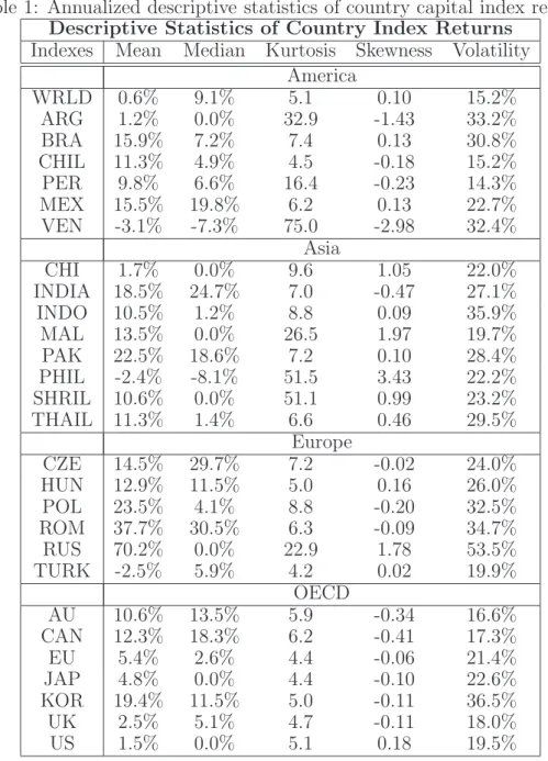
Table 1 shows descriptive sample statistics of the country index returns. The empirical return distributions are typically skewed and fat tailed.
TABLE 1 HERE
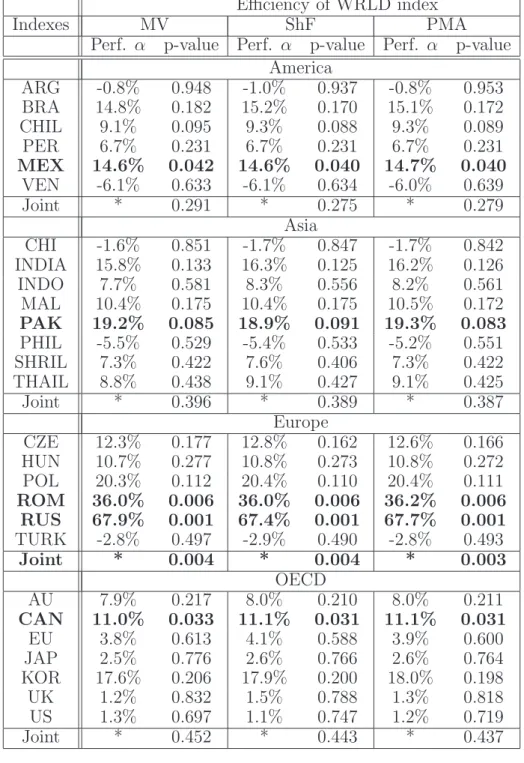
Table 2 shows the result of the world index (WRLD) efficiency tests. The table reports annualized regression intercept coefficients, which can be interpreted as performance measures (see discussion in section 5), and signif-icance levels of the mean-variance (MV), mean-expected shortfall (ShF), and the mean-PMA CRR (PMA) market efficiency tests with respect to inclusion of individual country indexes. The expected shortfall probability threshold
is chosen to be 5%, while probability thresholds for PMA CRR are taken at the levels of 5%, 10%, 15%, 20%, and 25% with equal weights of 20%. Significance levels of joint spanning tests for inclusion of country groups as a whole are reported in the table as well.
TABLE 2 HERE
We see that the market efficiency tests with different risk measures (vari-ance, expected shortfall, and PMA CRR) lead to similar conclusions in terms of both performance measures and significance levels. In most cases the mar-ket efficiency of the WRLD index cannot be rejected at the usual significance levels. A strong rejection of the efficiency hypothesis is observed for Mexico, Romania, Russia, and Canada (5% significance level). The capital indexes of these countries significantly outperform the world market index at the 5% significance level. Indeed, Russian and Romanian markets have shown a significant growth over the past decade. The spanning hypothesis is also rejected for Pakistan at the 10% significance level.
The performanceα’s reported in the table for the mean-variance efficiency tests are, in fact, Jensen’s α’s. The rest of the performance measures (for mean-CRR efficiency) have a similar interpretation. The results of Table 2 indicate that Romanian and Russian capital market indexes outperform the world market index approximately by 36% and 68%, respectively. Moreover, this outperformance is statistically significant at the 1% significance level.
The fact that the mean-CRR spanning tests perform at similar signifi-cance levels with the mean-variance spanning tests is encouraging. It shows that the mean-CRR spanning tests for country indexes work reasonably well. Moreover, for a moderate levels of skewness and kurtosis in the index return distributions the different risk measures are statistically equivalent and can be used interchangeably. This is in line with findings in Polbennikov and Me-lenberg (2005) who perform a systematic comparison of the mean-variance and the mean-CRR approaches in portfolio management. De Giorgi and Post (2004), who test mean-variance and mean-CRR efficiency of the US market index for the beta and momentum portfolios, obtain similar results: the mean-variance and mean-CRR performance measures as well as the test
statistics are comparable.13
6.2
Testing for mean-CRR spanning in portfolios of
credit instruments
Our second example concerns portfolios of credit instruments. In particular, we consider collateralized debt obligations (CDO) as elementary entries of the portfolio. This example is chosen for two reasons. First, since CDO return distributions are not symmetric the mean-variance and mean-CRR market efficient portfolios are likely to be different. As a result, the outcomes of the spanning tests might be different as well. Second, CDO tranches are becoming very popular financial instruments among investors, for example, hedge funds, insurance companies, etc. The past several years have seen an increasingly growing market for CDO tranches. This means that the problem of finding an optimal portfolio of CDOs is relevant for practical applications. The mean-variance approach might not be good idea in this case due to significantly asymmetric returns.
A collateralized debt obligation (CDO) is a structure of fixed income se-curities whose cash flows are linked to the incidence of default in a pool of debt instruments. These debts may include loans, emerging market corpo-rate or sovereign debt, and subordinate debt from structured transactions. The fundamental idea behind a CDO is that one can take a pool of default-able bonds or loans and issue securities whose cash flows are backed by the payments due on the loans or bonds. Using a rule for prioritizing the cash flow payments to the issued securities, it is possible to redistribute the credit risk of the pool of assets to create securities with a variety of risk profiles. In our example we consider the simplest case of investing in securities linked to the total pool of the underlying debt, while receiving a fixed interest payment in exchange.
In the industry the analysis of CDOs is usually exclusively based on the-oretical models. This is due to the fact that historical data on defaults, and especially joint defaults, is very sparse. Another reason is that the
speci-13
The test by De Giorgi and Post (2004), however, seems to ignore the effect of the non-parametric estimation of the pricing kernel.
fication of the full joint default probabilities is too complex: for example, for a CDO with 50 obligors there are 250 joint default events. CDO models differ in their complexity: while some of them admit analytical solutions for loss distribution functions, others require Monte-Carlo simulation techniques. However, as soon as one wants to construct an optimal mean-risk portfolio from several CDOs, no closed form solution is usually available. Therefore, a Monte-Carlo simulation is the only alternative. In our example, we use a simple one factor large homogeneous portfolio model to construct the return distributions of the CDOs.14 Here we briefly outline the model.
The model assumes that a portfolio of loans consists of a large number of credits with the same default probability p. In addition, it is assumed that the default of a firm (obligor) is triggered when the normally distributed value of its assets Vn(T) falls below a certain level K. Without loss of generality
we can standardize the developments of the firm values such that Vn(T) ∼ N(0,1). In this case the default barrier level is the same for all obligors and equals K = Φ−1(p). To introduce a default correlation structure it is assumed that the firm values are driven by a factor model
Vn(T) =√̺Y +
p
1−̺ǫn,
whereY is the systematic factor for all obligors in the pool of credits, andǫn
is the idiosyncratic risk of a firm. The higher the correlation coefficient̺, the higher the probability of a joint default in the pool. Notice that, conditional on the factorY, defaults are independent. The individual default probability conditional on the realization yof the systematic factor Y is
p(y) = Φ Φ−1(p)−√̺y √ 1−̺ .
Conditional on the realization y of Y, the individual defaults happen inde-pendently from each other. Therefore, in a very large portfolio, as we assume to be the case, the law of large numbers ensures that the fraction of oblig-ors that actually defaults is almost surely equal to the individual default probability.
14
We use a simplified form of the firm’s value model due to Vasicek (1997). Similar approach is used in Belkin et al. (1998) and Finger (1999).
For purposes of our analysis we simulate returns of three CDOs using the described one factor model. The steps that we take are as follows:
• We simulate 10,000 realizations of three factors (y1i, y2i, y3i) from the
three-variate standard normal distribution with the identity correlation matrix.15
• From the simulated factors we generate fractions of obligors that actu-ally default in the pool j ={1,2,3}using the formula
xji = Φ Φ−1(p j)−√̺jyji p 1−̺j !
with individual default probabilities pj, j = {1,2,3} of 2.5%, 5%, and
7.5%; and default correlations ̺j, j ={1,2,3}of 0.15, 0.1, and 0.05.
• Finally, for each CDO j we obtain the returns Rji Rji = (1 +rj)(1−xji)−1,
where rj is the risk premium for holding pool j of defaultable obligors.
We choose these risk premiums to be 4%, 10%, and 12%, correspond-ingly.
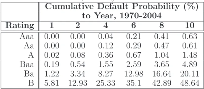
Even though the parameter choice in our simulation may seem ad-hoc, there are two reasons which make it plausible for a realistic situation. First, depending on the credit rating and the investment horizon, individual de-fault probabilities can vary in a wide range from 0.00% (for one year dede-fault probability of an Aaa rated company) to almost 50% (for ten years default probability of a B rated company), according to Moody’s, see Table 3 with historical cumulative default probabilities for the period 1970-2004. The de-fault probabilities that we choose fall in this range. Second, it is possible to redistribute the credit risk of the pool of assets to create securities with a va-riety of risk profiles, which makes many possible combinations of parameters justified.
15
In principle, it is possible to make returns on the 3 CDOs dependent by introducing positive or negative correlations among the factors.
TABLE 3 HERE
Table 4 shows descriptive statistics of the simulated returns of the three CDOs. The distributions of the returns are substantially skewed and fat tailed. The CDO with the smallest default correlation among obligors is the closest to the normal distribution.
TABLE 4 HERE
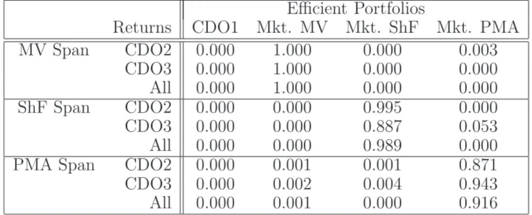
From the simulated credit pool returns we construct three market portfo-lios:16 mean-variance (MV), mean-expected shortfall (ShF) and mean-PMA CRR (PMA). In addition, we consider returns of CDO1 hypothesizing its market efficiency. The probability threshold for expected shortfall is chosen to be 5%. The probability thresholds for PMA CRR measure are chosen to be 5%, 10%, 15%, 20%, and 25% with equal weights of 20%. For these four portfolios (CDO1, MV, ShF, and PMA) we perform mean-variance, mean-expected shortfall, and mean-CRR PMA spanning tests with respect to inclusion of CDO2 and CDO3. Table 5 reports significance levels of these tests.
TABLE 5 HERE
The results indicate a statistical difference between mean-variance and mean-CRR market portfolios. For the mean-CRR market portfolios (Mkt. ShF and Mkt. PMA), the mean-variance spanning tests result in strong rejection. At the same time, for the mean-variance market portfolio (Mkt. MV) mean-CRR spanning tests result in rejection as well. The difference between the mean-expected shortfall market portfolio (Mkt. ShF) and the mean-PMA CRR market portfolio (Mkt. PMA) with respect to the inclusion of CDO2 and CDO3 turns out to be significant as well.
In this exercise the mean-variance and the mean-CRR spanning tests do not produce similar results any more. The reason is the asymmetrically distributed returns. Skewness of the returns makes the variance a bad risk measure from the point of view of a CRR investor. Therefore, the mean-variance optimal portfolio is not recognized as a mean-CRR efficient one by
16
the mean-CRR spanning test. This exercise demonstrates the applicability of the mean-CRR spanning test to portfolios of credit instruments or other portfolios with comparable characteristics. It shows that the correct choice of the risk measure becomes increasingly important for assets with asymmetric returns.
7
Conclusion
In this paper we consider coherent regular risk (CRR) measures as an alter-native to the conventional variance in a mean-risk optimal portfolio problem. Following trends in the recent literature on expected shortfall we derive useful properties of CRR measures. In particular, expressions for risk contributions and the Hessian of a CRR measure are obtained.
Our main contribution is the regression-based test for mean-CRR span-ning. We show that this test can be performed in the spirit of Huberman and Kandel (1987) as a significance test of the intercept coefficient in a semi-parametric instrumental variable regression. The instrument in this regres-sion is a functional, depending on a certain choice of the CRR measure.
We derive the limit distribution of the regression intercept coefficient to test for mean-CRR spanning. The resulting asymptotic covariance matrix is the variance of the usual IV estimator with an adjustment for the non-parametric part. In case of mean-expected shortfall or mean-PMA CRR portfolios this adjustment is likely to be negligible so that the non-parametric part can be ignored. Further, we illustrate how the estimation error in the mean-CRR portfolio weights can be incorporated in the spanning test.
The instrumental variable in the semi-parametric IV regression can be used to construct a stochastic discount factor of a CRR version of the CAPM. In particular, we show that this stochastic discount factor is an affine function of this instrumental variable. This allows for an alternative interpretation of our spanning test in terms of a performance measure similar in spirit to the way the performance measure Jensen’s αis related to the mean-variance spanning test.
Finally, as an empirical application, we use the mean-CRR spanning test to test for CRR efficiency of the world capital market index. In particular,
we test for mean-expected shortfall and mean-PMA CRR efficiency with respect to the inclusion of individual country indexes. We find that the mean-CRR and mean-variance spanning tests produce similar significance levels. In addition we consider spanning tests for simulated returns of simplistic CDOs. We show that due to asymmetry of the return distributions mean-variance and mean-CRR spanning tests produce statistically different results.
A
Proof of proposition 1
First, notice that expected shortfall of the portfolio returnZcan be expressed as
sα(Z) =−αE[ZI(Fz(Z)≤α)],
whereI(A) is the usual indicator function. This means that a CRR measure of the portfolio Z is ρ(θ) = − Z 1 0 α−1E[ZI(Fz(Z)≤α)]dφ(α) = −E Z Z 1 0 α−1I(Fz(Z)≤α)dφ(α) = −E Z Z 1 Fz(Z) α−1dφ(α) .
The distribution function Fz(·) is continuously differentiable with respect to
portfolio weights θ since the distribution of the returns R has a continuous density. Therefore, we can calculate the risk contributions of a CRR measure in a straightforward way. Notice, that portfolio Z =R′θ and its distribution functionFz depend on the portfolio weightsθ. Then, applying the chain rule
to the expression for a CRR measure ρ(θ), we obtain
∇θρ(θ) = −∇θE Z Z 1 Fz(Z) α−1dφ(α) (27) = −E R Z 1 Fz(Z) α−1dφ(α)−Zφ ′(F z(Z)) Fz(Z) (fz(Z)R+∇θFz(s)|s=Z) .
To finish the derivation we need to calculate the gradient∇θFz(s). It suffices
byθj the portfolio weight of assetRjand byθ−j the vector of portfolio weights
of the rest of the assets, which we denote byR−j. Further, let Z−j =R′−jθ−j
be the portfolio of assets R excluding asset j. Denote by Fz−j|Rj and fz−j|Rj
the conditional probability and density functions of return Z−j conditional
on return Rj. Then we can express the cumulative probability function Fz
of portfolio Z though the expectation of the conditional probability Fz−j|Rj
Fz(s) =E[I(R′θ≤s)] = E EI(R′−jθ−j ≤s−Rjθj) Rj = EFz−j|Rj(s−Rjθj) .
Now the calculation of the derivative of Fz(s) with respect to weight θj is
straightforward ∂Fz(s) ∂θj = −Efz−j|Rj(s−Rjθj)Rj =−Efz|Rj(s)Rj = − Z +∞ −∞ fz,Rj(s, Rj) fRj(Rj) RjdFRj(Rj) =−fz(s)E[Rj|Z =s],
where fz|Rj is the conditional density function of the portfolio return Z
con-ditional on returnRj of the assetj, andfz,Rj is their joint probability density
function. Stacking the components into one vector yields
∇θFz(s) =−fz(s)E[R|Z =s],
Then, substituting this expression into equation (27), we obtain the result for the CRR risk contributions
∇θρ(θ) = −E R Z 1 Fz(Z) α−1dφ(α)−Zφ ′(F z(Z)) Fz(Z) (fz(Z)R−fz(Z)E[R|Z]) = −E R Z 1 Fz(Z) α−1dφ(α) ,
B
Proof of proposition 2
The proof is straightforward
∇2θρ(θ) = −∇θE R Z 1 Fz(Z) α−1dφ(α) = E Rφ ′(F z(Z)) Fz(Z) (fz(Z)R′ +∇θ Fz(s)|s=Z) = E φ′(Fz(Z))fz(Z) Fz(Z) (RR′ −RE[R′|Z]) = E φ′(Fz(Z))fz(Z) Fz(Z) Cov(R|Z) .
C
Influence function of semi-parametric IV
regressors
As discussed in subsection 4.1, the derivation of the limit distribution of parameters in semi-parametric IV regression (13) requires the derivation of the influence function of the functional
φ2(F) =
Z
ǫν′(F(Z))dF(z, ǫ). (28)
We refer to van der Vaart (1998) and Newey (1994) for the methodology and appropriate regularity conditions. The idea is that the functional delta method applies to a functionalφ2(·) :DF →Rsatisfying Hadamard
differen-tiability, so that for any square root consistent estimator Fn of the function F √ n(φ2(Fn)−φ2(F)) = 1 √ n n X i=1 ψ2(zi, ǫi) +op(1), ψ2(z, ǫ) = d dt[φ2((1−t)F +tδx)]t=0.
The function ψ2(F) is known as the influence function of the functional φ2. We rewrite the functional (28) as an expectation:
where the random variableǫstands for the error term of the linear model (9),
Z is the random variable corresponding to the return on the CRR market portfolio, and F is the cdf of Z.
Denote by g(Z) the projection ofǫ onZ, i.e.,g(Z) =E[ǫ|Z]. Introduce a ”misspecified” joint distribution function Fθ(z, ǫ) along the path θ, such
that F0 is the true distribution function. Then we can calculate the influ-ence function from the pathwise derivative of the given functional, using the pathwise derivative (see Newey (1994)):
dEθ[gθ(Z)ν′(Fθ)] dθ = ∂Eθ[g(Z)ν′(F)] ∂θ + ∂E[gθ(Z)ν′(F)] ∂θ + ∂E[g(Z)ν′(Fθ)] ∂θ ,
where we denote Fθ as the ”misspecified” marginal distribution function of Z corresponding to the ”misspecification” of the joint distribution function
Fθ(z, ǫ), gθ(Z) as the ”misspecified” conditional expectation of ǫ given Z, Eθ[·] as the expectation under the ”misspecified” distribution Fθ(z, ǫ).
For-mally: Fθ(z) = z Z −∞ ∞ Z −∞ dFθ(s, t), gθ(z) = ∞ Z −∞ tdFθ(t|Z =z), Eθ[·] = ∞ Z −∞ ∞ Z −∞ ·dFθ(s, t).
From the expression for the pathwise derivative we can see that the influence function of the functional (28) can be represented as a superposition of three influence functions of the misspecified functionals:
ψ2(z, ǫ) =ψA(z, ǫ) +ψB(z, ǫ) +ψC(z, ǫ), with dEθ[gθ(Z)ν′(Fθ)] dθ θ=0 =E ψ2(Z, ǫ) ∂lndFθ ∂θ θ=0 .
Further, we calculate the separate pathwise derivative and find the influ-ence function of the functional (28). The first part of the influinflu-ence function is easy to find: ∂Eθ[g(Z)ν′(F)] ∂θ =E g(Z)ν′(F)∂lndFθ ∂θ ,
so that the first part of the influence function is
ψA(z, ǫ) =g(z)ν′(F (z)) (29)
For the second part, we find, using the chain rule and the definition of the projection gθ: ∂E[gθ(Z)ν′(F)] ∂θ = ∂Eθ[gθ(Z)ν′(F)] ∂θ − ∂Eθ[g(Z)ν′(F)] ∂θ = ∂Eθ[(ǫ−g(Z))ν ′(F)] ∂θ = E (ǫ−g(Z))ν′(F)∂lndFθ ∂θ ,
so that the second part of the influence function is
ψB(z, ǫ) = (ǫ−g(z))ν′(F (z)). (30)
To calculate the last part of the influence function we directly apply the definition of the influence function to the functional E[g(Z)ν′(Fθ)]:
ψC(z, ǫ) = d dt Z g(s)ν′((1−t)F +tδz)dF t=0 = (31) = Z g(s) (δz−F)dν′(F).
The influence function of the functional (28) is the superposition of the three calculated influence functions (29),(30) and (31):
ψ(z, ǫ) = ψA(z, ǫ) +ψB(z, ǫ) +ψC(z, ǫ) = χ(z, ǫ)−E[χ(Z, ǫ)], (32) χ(z, ǫ) = ǫν′(F (z)) + ∞ Z z g(s)dν′(F (s)). (33)
Substituting the expression for Choquet distortion pdf ν′(t) from (3) into
(33) we obtain the final result
χ(z, ǫ) =
Z 1
F(z)
ǫ−E[ǫ|Z =F−1(α)]α−1dφ(α).
D
Influence function of CRR efficient
port-folio weights
Results on the asymptotic distribution of mean-CRR efficient portfolio weights are obtained in companion paper by Polbennikov and Melenberg (2005). Here we briefly restate the results without the derivation details.
Let Re be a vector of the asset excess returns (R
1 − rf, . . . , Rp −rf),
and Z =rf +Re′θ be a portfolio of these assets. The mean-CRR portfolio
problem can be formulated as min θ∈RpE −Z Z 1 Fz(Z) α−1dφ(α) s.t. E[Z] = m,
wheremis the expected return on the efficient portfolio. From an economet-ric perspective this problem is a standard constrained extremum estimation problem, so that the limit distribution of resulting portfolio weights can be found in the usual way, see Gourieroux and Monfort (2005) and Polbennikov and Melenberg (2005). The asymptotic distribution results can be equiva-lently expressed through the estimator influence function. Here we report the final results. The influence function of the mean-CRR optimal portfolio weighs is ξ(Re, Z) = H−1 " bCC′H−1−Ip −bC #′" ψ∇f −λψ∇g ψg # ,
where we use notations similar with Polbennikov and Melenberg (2005). The vector C stands for the gradient of the constraint function with respect to portfolio weighs C =E[Re]. The scalar λ is the Lagrange multiplier
λ=−E ι′Re Z 1 Fz(Z) α−1dφ(α) (ι′E[Re])−1,
where ι stands for a (p×1) vector of ones. The matrix H is the Hessian of the objective function with respect to portfolio weights evaluated at the optimum H =E φ′(F z(Z))fz(Z) Fz(Z) Cov(Re|Z) .
The functions ψ∇f and ψ∇g are the influence functions of the objective and
constraint function gradient functionals, respectively. The expressions for them are given by
ψ∇f = χ∇f −E[χ∇f], χ∇f = − Z 1 Fz(Z) Re−ERe|Z =F−1(α)α−1dφ(α), ψ∇g = Re−E[Re].
The function ψg is the influence function of the constraint functional, ψg = Z −m. Finally, the scalar b is a notation
b = C′H−1C−1.
The asymptotic distribution of the mean-CRR optimal portfolio weights is
√
nbθ−θ→dN(0, E[ξξ′]).
D.1
Expected shortfall
The asymptotic result for the mean-expected shortfall optimal weights is a special case of the mean-CRR weighs considered above withφ(α) = I(α≥τ). Substituting this expression into the corresponding formulas yields
λ = −τ−1E[ι′ReI(Fz(Z)≤τ)] (ι′E[Re]) −1 , H = = f(F −1 z (τ)) τ Cov(R e |Z =Fz−1(τ)), χf = −τ−1I(Fz(Z)≤τ) Re−E[Re|Z =Fz−1(τ)] .
The expression for the influence function of the mean-expected shortfall port-folio weights follows immediately.
D.2
Point mass approximation (PMA) of a CRR
The point mass approximation of a CRR measure suggested by Bassett et al. (2004) takes φ(α) = m X k=1 φkI(α≥τk).
This is also a special case of a CRR measure. Therefore, the derived asymp-totic results for a mean-CRR portfolio weights still apply. We have
λ = − m X k=1 φkτk−1E[ι′ReI(Fz(Z)≤τk)] (ι′E[Re])−1, H = E∇2θf= m X k=1 φkτk−1f(Fz−1(τk))Cov(Re|Z =Fz−1(τk)), χf = − m X k=1 φkτk−1I(Fz(Z)≤τk) Re−E[Re|Z =Fz−1(τk)] .
The expression for the influence function of the mean-PMA CRR portfolio weights follows immediately.
References
C. Acerbi. Spectral measures of risk: A coherent representation of subjective risk aversion. Journal of Banking & Finance, 26:1505–1518, 2002.
C. Acerbi and D. Tasche. Expected shortfall: A natural coherent alternative to value at risk. Economic Notes, 31:379–388, 2002.
P. Artzner, F. Delbaen, J.-M. Eber, and D. Heath. Coherent measures of risk. Mathematical Finance, 9:203–228, 1999.
I. Barrodale and F. D. K. Roberts. Solution of an overdetermined system of equations in the l1 norm. Communications of the ACM, 17:319–320, 1974. G. W. Bassett, R. W. Koenker, and G. Kordas. Pessimistic portfolio alloca-tion and Choquet expected utility. Journal of Financial Econometrics, 2: 477–492, 2004.
B. Belkin, S. Suchover, and L. Forest. A one-parameter representation of credit risk and transition matrices. Credit Metrics Monitor, 1:46–56, 1998. D. Bertsimas, G. J. Lauprete, and A. Samarov. Shortfall as a risk measure: Properties, optimization and applications. Journal of Economic Dynamics & Control, 28:1353–1381, 2004.
M. Britten-Jones. The sampling error in estimates of mean-variance efficient portfolio weights. Journal of Finance, 54:655–671, 1999.
Z. Chen and P. J. Knez. Portfolio performance measurement: Theory and applications. The Review of Financial Studies, 9:511–555, 1996.
R. E. Cumby and J. D. Glen. Evaluating the performance of international mutual funds. Journal of Finance, 45:497–521, 1990.
E. De Giorgi. Reward-risk portfolio selection and stochastic dominance. Jour-nal of Banking & Finance, 29:895–926, 2005.
E. De Giorgi and T. Post. Second order stochastic dominance, reward-risk portfolio selection and the CAPM. Working Paper, University of Lugano, 2004.
F. Delbaen. Coherent risk measures on general probability spaces. Working Paper, 2000.
F. A. DeRoon and T. E. Nijman. Testing for mean-variance spanning: a survey. Journal of Empirical Finance, 8:111–155, 2001.
C. C. Finger. Conditional approaches for credit metrics portfolio distribu-tions. Credit Metrics Monitor, 2:14–33, 1999.
H. F¨ollmer and A. Schied. Advances in Finance and Stochastics, chapter Ro-bust Preferences and Convex Measures of Risk, pages 111–155. Springer-Verlag, Berlin, 2002.
C. Gourieroux and A. Monfort. The econometrics of efficient portfolios. Journal of Empirical Finance, 12:1–41, 2005.
G. Huberman and S. Kandel. Mean-variance spanning. Journal of Finance, 52:873–888, 1987.
M. Kalkbrener. An axiomatic approach to capital allocation. Mathematical Finance, 15:425–437, 2005.
J. Kerkhof and B. Melenberg. Backtesting for risk-based regulatory capital. Journal of Banking & Finance, 28:1845–1865, 2004.
R. W. Koenker and V. D’Orey. Computing regression quantiles. Journal of Royal Statistical Society Series C, 36:383–393, 1987.
S. Kusuoka. On law invariant coherent risk measures. Advances in Mathe-matical Economics, 3:83–95, 2001.
H. M. Markowitz. Portfolio selection. Journal of Finance, 7:77–91, 1953. W. K. Newey. The asymptotic variance of semiparametric estimators.
Econo-metrica, 62:1349–1382, 1994.
W. Ogryczak and A. Ruszczy´nski. Dual stochastic dominance and related mean-risk models. SIAM Journal on Optimization, 13:60–78, 2002. C. S. Pedersen and S. E. Satchell. An extended family of financial risk
measures. The Geneva Papers on Risk and Insurance Theory, 23:89–117, 1998.
S. Polbennikov and B. Melenberg. Mean-coherent regular risk and mean-variance approaches in portfolio selection: an empirical comparison. Work-ing Paper, Tilburg University, 2005.
S. Portnoy and R. W. Koenker. The Gaussian hare and Laplacian tortoise: Computability of squared-error versus absolute-error estimators.Statistical Science, 12:299–300, 1997.
J. Quiggin. A theory of anticipated utility. Journal of Economic Behavior and Organization, 3:225–243, 1982.
F. P. Ramsey. The Foundations of Mathematics and Other Logical Essays, chapter Truth and Probability. Harcourt Brace, 1931.
R. T. Rockafellar and S. Uryasev. Optimization of conditional value-at-risk. The Journal of Risk, 2:21–41, 2000.
L. J. Savage. Foundations of Statistics. Wiley, 1954.
D. Schmeidler. Subjective probability and expected utility without additivity. Econometrica, 57:571–587, 1989.
D. Tasche. Risk contributions and performance measurement. Working Pa-per, 1999.
D. Tasche. Expected shortfall and beyond. Journal of Banking & Finance, 26:1519–1533, 2002.
A. Tversky and D. Kahneman. Advances in prospect theory: Cumulative representation of uncertainty. Journal of Risk and Uncertainty, 5:297–323, 1992.
A. W. van der Vaart. Asymptotic Statistics. Cambridge University Press, 1998.
O. A. Vasicek. The loan loss distribution. Working Paper, KMV Corporation, 1997.
J. von Neumann and O. Morgenstern. Theory of Games and Economic Be-havior. Princeton, 1944.
P. Wakker and A. Tversky. An axiomatization of cumulative prospect theory. Journal of Risk and Uncertainty, 7:147–176, 1993.
M. E. Yaari. The dual theory of choice under risk. Econometrica, 55:95–115, 1987.
Table 1: Annualized descriptive statistics of country capital index returns.
Descriptive Statistics of Country Index Returns
Indexes Mean Median Kurtosis Skewness Volatility America WRLD 0.6% 9.1% 5.1 0.10 15.2% ARG 1.2% 0.0% 32.9 -1.43 33.2% BRA 15.9% 7.2% 7.4 0.13 30.8% CHIL 11.3% 4.9% 4.5 -0.18 15.2% PER 9.8% 6.6% 16.4 -0.23 14.3% MEX 15.5% 19.8% 6.2 0.13 22.7% VEN -3.1% -7.3% 75.0 -2.98 32.4% Asia CHI 1.7% 0.0% 9.6 1.05 22.0% INDIA 18.5% 24.7% 7.0 -0.47 27.1% INDO 10.5% 1.2% 8.8 0.09 35.9% MAL 13.5% 0.0% 26.5 1.97 19.7% PAK 22.5% 18.6% 7.2 0.10 28.4% PHIL -2.4% -8.1% 51.5 3.43 22.2% SHRIL 10.6% 0.0% 51.1 0.99 23.2% THAIL 11.3% 1.4% 6.6 0.46 29.5% Europe CZE 14.5% 29.7% 7.2 -0.02 24.0% HUN 12.9% 11.5% 5.0 0.16 26.0% POL 23.5% 4.1% 8.8 -0.20 32.5% ROM 37.7% 30.5% 6.3 -0.09 34.7% RUS 70.2% 0.0% 22.9 1.78 53.5% TURK -2.5% 5.9% 4.2 0.02 19.9% OECD AU 10.6% 13.5% 5.9 -0.34 16.6% CAN 12.3% 18.3% 6.2 -0.41 17.3% EU 5.4% 2.6% 4.4 -0.06 21.4% JAP 4.8% 0.0% 4.4 -0.10 22.6% KOR 19.4% 11.5% 5.0 -0.11 36.5% UK 2.5% 5.1% 4.7 -0.11 18.0% US 1.5% 0.0% 5.1 0.18 19.5%
Table 2: Efficiency tests of the Morgan Stanley world capital index (WRLD). The table reports performance measures α’s and p-values of the mean-variance (MV), mean-expected shortfall (ShF) and mean-PMA CRR (PMA) spanning tests. Probability threshold for expected shortfall is 5%. Probabil-ity thresholds for PMA CRR are 5%, 10%, 15%, 20%, and 25% with equal weights of 20%.
Efficiency of WRLD index
Indexes MV ShF PMA
Perf. α p-value Perf. α p-value Perf. α p-value America ARG -0.8% 0.948 -1.0% 0.937 -0.8% 0.953 BRA 14.8% 0.182 15.2% 0.170 15.1% 0.172 CHIL 9.1% 0.095 9.3% 0.088 9.3% 0.089 PER 6.7% 0.231 6.7% 0.231 6.7% 0.231 MEX 14.6% 0.042 14.6% 0.040 14.7% 0.040 VEN -6.1% 0.633 -6.1% 0.634 -6.0% 0.639 Joint * 0.291 * 0.275 * 0.279 Asia CHI -1.6% 0.851 -1.7% 0.847 -1.7% 0.842 INDIA 15.8% 0.133 16.3% 0.125 16.2% 0.126 INDO 7.7% 0.581 8.3% 0.556 8.2% 0.561 MAL 10.4% 0.175 10.4% 0.175 10.5% 0.172 PAK 19.2% 0.085 18.9% 0.091 19.3% 0.083 PHIL -5.5% 0.529 -5.4% 0.533 -5.2% 0.551 SHRIL 7.3% 0.422 7.6% 0.406 7.3% 0.422 THAIL 8.8% 0.438 9.1% 0.427 9.1% 0.425 Joint * 0.396 * 0.389 * 0.387 Europe CZE 12.3% 0.177 12.8% 0.162 12.6% 0.166 HUN 10.7% 0.277 10.8% 0.273 10.8% 0.272 POL 20.3% 0.112 20.4% 0.110 20.4% 0.111 ROM 36.0% 0.006 36.0% 0.006 36.2% 0.006 RUS 67.9% 0.001 67.4% 0.001 67.7% 0.001 TURK -2.8% 0.497 -2.9% 0.490 -2.8% 0.493 Joint * 0.004 * 0.004 * 0.003 OECD AU 7.9% 0.217 8.0% 0.210 8.0% 0.211 CAN 11.0% 0.033 11.1% 0.031 11.1% 0.031 EU 3.8% 0.613 4.1% 0.588 3.9% 0.600 JAP 2.5% 0.776 2.6% 0.766 2.6% 0.764 KOR 17.6% 0.206 17.9% 0.200 18.0% 0.198 UK 1.2% 0.832 1.5% 0.788 1.3% 0.818 US 1.3% 0.697 1.1% 0.747 1.2% 0.719 Joint * 0.452 * 0.443 * 0.437
Table 3: Moody’s cumulative default probabilities by letter rating from 1-10 years, 1970-2004. For more details see Default and Recovery Rates of Corporate Bond Issuers, 1920-2004, Special Comment, Moody’s Investors Service, Global Credit Research, January 2005.
Cumulative Default Probability (%) to Year, 1970-2004 Rating 1 2 4 6 8 10 Aaa 0.00 0.00 0.04 0.21 0.41 0.63 Aa 0.00 0.00 0.12 0.29 0.47 0.61 A 0.02 0.08 0.36 0.67 1.04 1.48 Baa 0.19 0.54 1.55 2.59 3.65 4.89 Ba 1.22 3.34 8.27 12.98 16.64 20.11 B 5.81 12.93 25.33 35.1 42.89 48.64
Table 4: Descriptive statistics of the simulated CDO returns. Sample cor-relation matrix is given at the bottom of the table. Returns are simulated from the one-factor large homogeneous portfolio model.
Simulation Parameters Def. Prob.: 2.5% 5% 7.5%
Def. Corr.: 0.15 0.1 0.05 Risk Prem.: 4% 10% 12% Sample Return Statistics Min.: -27.00% -30.80% -16.80% 1st Qu.: 0.64% 2.78% 1.58% Median: 2.25% 5.47% 4.20% Mean: 1.40% 4.52% 3.60% 3rd Qu.: 3.16% 7.27% 6.29% Max.: 3.99% 9.83% 10.80% Std. Dev. 2.72% 3.86% 3.68% Skew. -2.63 -1.75 -1.03 Kurtos. 13.85 8.35 4.62 CDO1 1.00 0.01 0.00 CDO2 0.01 1.00 0.01 CDO3 0.00 0.01 1.00