Bachelor Thesis Performance comparison of heuristic algorithms in routing optimization of sequencing traversing cars in a warehouse

(1)

Bachelor Thesis

Performance comparison of heuristic algorithms in routing

optimization of sequencing traversing cars in a warehouse

Minh Hoang Technische Universität Hamburg-Harburg

supervised by: Prof. Dr. Sibylle Schupp Institute for Software Systems TUHH

(2)

2

Acknowledgement

My most sincere thanks go to Prof. Dr. Sibylle Schupp, who has inspired and given me this previous chance to write this thesis on an interesting topic. I also owe many thanks to Prof. Dr. Ralf Möller, who is the second examiner for my thesis.

My great gratitude goes to Mr. Rainer Marrone, who has motivated and guided me through all the steps to accomplish this thesis, who has supported me throughout this very first thesis of mine with his patience and knowledge whilst allowing me the room to work in my own way.

(3)

3

Declaration

I hereby confirm that I have authored my bachelor thesis with the title

"Performance comparison of heuristic algorithms in warehouse transport optimization"

independently and without use of others than the indicated resources. All passages taken out of publications or other sources are marked as such.

Eidesstattliche Erklärung

Hiermit versichere ich, dass ich meine Masterthesis mit dem Thema

"Performance comparison of heuristic algorithms in warehouse transport optimization"

selbstständig verfasst und keine anderen als die angegebenen Quellen und Hilfsmittel benutzt habe.

Hamburg, April 10, 2010 Minh Hoang

(4)

4

Abstract

This thesis aims at comparing the performance of heuristics algorithms used to solve the "Sequencing Traversing Cars in a Warehouse Problem" (STCP) as an extension of the classic "Traveling Salesman Problem" (TSP). Algorithms to benchmark are Genetic Algorithm and Ant-Colony Algorithm, Greedy Algorithm, and Greedy Algorithm with 2-op Optimization. STCP has both similar and different features from the "Travelling Salesman Problem” (TSP). To adapt the solutions of TSP in STCP, it is necessary to analyze the similarities and differences between the two problems.

In order to implement solutions for STCP and a platform for numerical comparison of the applied algorithms, this thesis proposes an UML-model of a simple warehouse system and programming test bench used for comparing solutions of STCP.

Keywords: Optimization algorithms, TSP, Sequencing Traversing Car, Pick-up and Delivery, Greedy Algorithm, Ant-Colony Algorithm, Genetic Algorithm.

(5)

5

Chapter 1 Introduction

1.1.Motivation

The "Travelling Salesman Problem" has been a popular research topic among experts and scholars of mathematics and computer science. With the goal of minimizing the total travel distance of the salesman in Travelling Salesman Problem (TSP), TSP's solutions can be applied to a wide range of discrete optimization problems. Reducing travel cost of transportation and logistics distribution are one of typical applications of TSP.

Transportation optimization is the most natural application of TSP, in which TSP can play the role of reducing travel cost. Büchter & Novoa [1] suggested that the Sequencing Traversing-Cars in a Warehouse Problem can be solved as an extension of TSP. They also provided statistical comparison between solutions used Greedy Algorithm and Ant-Colony Optimization (ACO). The comparison has shown that ACO is a promising technique to incorporate in algorithms for warehouse traffic sequencing. It is a temptation to apply other heuristic algorithms used to solve TSP in Sequencing Traversing Car in A Warehouse Problem (STCP) and compare their performances in aspects of finding the most optimal tour and algorithm run-time.

1.2.Task description

This thesis analyzes characteristics and features of STCP and suggests a problem transformation from STCP to TSP. It also compares performances between two heuristic algorithms Ant-Colony Algorithms, Genetic Algorithm and with some other algorithms in solving STCP. Since STCP can be considered as a sub-problem or an extension of TSP. In order to adapt algorithms used in TSP in STCP, a test bench for

(8)

8

numerical comparison between applied algorithms in TSP and STCP is to be implemented.

1.3.Structure of the thesis

After Chapter 1 which provides a general idea of the thesis, Chapter 2 presents the description of the Sequencing Traversing Cars in a Warehouse with analyzing the features of the simple warehouse model used through the thesis. The Travelling Salesman Problem is also briefly introduced before suggesting a STCP-to-TSP transformation. The transformation will help apply TSP solutions to STCP.

Chapter 3 puts heuristic approaches in solving TSP in context. Two heuristic algorithms: Genetic Algorithm and Ant-Colony Algorithm and their applications in TSP are discussed in detail.

Chapter 4 is dedicated to present structures and workflows of the algorithms comparing test bench. The test bench imports solutions of TSP, transforms STCP to TSP and solves STCP. Design of the test bench as well as used programming frameworks and libraries are introduced in this Chapter 4.

In Chapter 5, a number of numerical and statistical comparisons between Greedy Algorithm, Genetic Algorithm and Ant-Colony Algorithm in STCP are performed in order to demonstrate the advantages and disadvantages of each algorithm. Chapter 5 also defines a list of experiments cases to tune optimal parameters of Ant-Colony System and Genetic Algorithm when they are applied to STCP.

The conclusion and summary is presented in Chapter 6 with a brief overview of implications for future work.

(9)

9

Chapter 2 Sequencing Traversing Cars in a

Warehouse

This chapter describes the Sequencing Traversing Cars in a Warehouse Problem. Features of a warehouse are analyzed in order to classify the problem into sub-problems like car loading problem, multi-Collecting Problem, Routing Problem, etc. This Chapter also provides an introduction of the Travelling Salesman Problem and discusses the similarities and differences between routing of a salesman and that of a traversing car in a warehouse.

2.1.Introduction

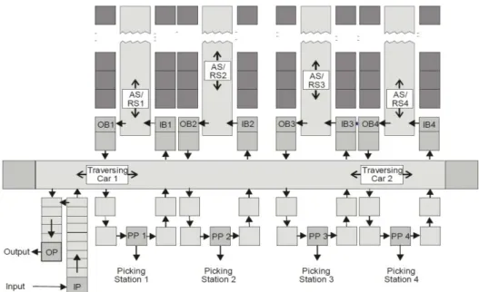
Figure 1: a simple warehouse model depicts a simple warehouse system.

(10)

10

The warehouse model has only one single input (IP) and output (OP) point, four picking stations (PP), four storage aisles which have single output buffer (OB) and input buffer (IB) for each. AS and RS are the Automatic storage and Retrieval systems. Goods in warehouse are transferred between aisles, input, output and picking stations through a traversing car (TC). In Figure 1, the arrow shows the direction of where goods should go.

The above warehouse system has great demands of goods delivery in daily workflow. There are orders for traversing cars for deliver goods from input point to storage aisles, from storage aisles to output point or picking stations, or directly from IP to OP in some specific cases. The main problem of as traversing car in a warehouse is how to minimize traveling distance between stations under considerations of available resources which can be stations’ storage buffer and capacity.

2.2.A simple Warehouse System

In this section, we are going to consider characteristics of the warehouse model mentioned in [1]. Main subjects of the simple warehouse system are storage units (aisle, picking point), retrieval units and picking units (car).

2.2.1. Storing capacity

A real warehouse system has its own limited capacity. The capacity can be seen roughly as how many items it can store. More exactly, the capacity should be the dedicated size and volume used for storing goods. In this warehouse model, each storing point has its own size, which defines the limits of total items weight and size it can store. The limited capacity of each storing point can be mathematically presented as a pair: capacity = (w, s) with w being how much weight one storing point can keep items in, and s being the volume of the storing point. The total weight of all items needed to be stored in one station is not allowed to exceed the specific capacity of a station. Together with weight and dimension of items, temperature requirements are also a problem of a warehouse. As we can see from Figure 1, which describes a warehouse system, each picking station, input/output point and input/output buffer of each aisle has their limited storing

(11)

11

capacity. The problem of how to make the most optimal use of the storing capacity brings us to the classic computer science problem: The Rucksack Problem.

2.2.2. Timing constraints

According to Büchter & Novoa [1], the authors have attempted to find the optimal tour for the traversing car in a warehouse with a set of delivery orders. In reality, the orders can come to the car continuously. If the traversing car can compute only the most optimal tour for just a subset of orders, then it is obviously not the global optimal tour. But in the normal workflow, picking orders can come at anytime, and the traversing car should not be idle until all orders come and then calculate the global optimal tour. For that reason, it is acceptable to choose a certain number of orders for the traversing car to serve. This number should be based on an estimation of how many orders coming during a certain time span, and how many orders each traversing car can serve in that time span.

Another timing constraint is the time when an item should be delivered to its destination. Even with the car which has the most optimal tour for sparing travelling cost, it may not make the most wanted tour. If each order has its own expected-delivery time, then the most important goal is that all these timing demands are fulfilled regardless of the whole tour distance.

2.2.3. Priority of picking order and item consolidation

In most cases of warehouse transportation, the First In First Out (FIFO) rule is used for a stream of delivery orders. . The FIFO paradigm is not appropriate for cases in which each order has its own priority. Packet consolidation can be seen as an example of a priority problem. Let us consider there is a huge item waiting at an output buffer of aisle A to delivery to output point. The huge item is actually a packet which is waiting for other items from stations B and C to consolidate before sending. It is obvious that delivery orders of items from B and C have higher priority than the delivery order from A in this case. To solve such a problem of delivery orders with priority, it is essential to define validation rules preventing conflicts between picking order. Moreover, the consolidation capacity of wrapping packet, as well as the size of each items in it, also need to be identified, which leads us back to the problem of storing capacity. Priority of picking orders can be decided by warehouse administrators.

(12)

12

2.2.4. Traversing Car and Order-Picking

Properties of the traversing car should be taking into consideration before analyzing the solutions to the transportation optimization in a warehouse. The properties can be: the number of traversing car, the speed of the car, the car's storing capacity and its collection ability. If the warehouse has more than one car, then a new occurring problem is how to avoid delivery conflicts when the two cars serve the same set of picking orders. If they serve different sets of order, the global information base of station temporary buffer need to be rapidly updated and informed to each car. In reality, a real car can contain one or more items for one delivery task. For example, a car serves an order from A to D, and then on its way to D it can collect items from B, C and brings them to C.

The term Order-picking is about delivery goods of traversing cars in a warehouse from/to storing units or picking point, input/output points. According [2], order-picking is the most intensive and expensive process in warehouses and distributed center. Following is an exemplary number of delivery orders in a warehouse:

Mail-order trade (very large) Pharmaceutical wholesale trade Food regional warehouse Producer electric household appliances Orders/day 190 000 4 000 780 350 Ordered items/day 650 000 105 000 300 000 6800

Table 1: Exemplary number of picking orders pro day in warehouses [3]

2.2.5. A warehouse model for performance comparison of routing algorithms

The main focus of this thesis is to compare the performance of applied heuristic algorithms in finding the most optimal tour for the traversing car in a warehouse. Therefore, a good evaluation function should be defined to benchmark the algorithms with each others. So far, this thesis has discussed characteristics of a real warehouse system including storing capacity, timing, priority, and properties of traversing car. If each property of the warehouse is a parameter in the evaluation function, the function is going to be very complex. It needs to fulfill all storing-capacity, timing, priority constraints and all properties of the traversing car. The biggest importance for the

(13)

13

routing problem is the travel distance of traversing cars. Thus we restrict some constraints for our STCP in order to retrieve a simple evaluation function which makes it easy to compare between applied solutions. Followings are the features of the warehouse model for our STCP:

• Every item has a same weight and volume to avoid the storing capacity problem mentioned in 2.2.1.

• Storing capacity is just about number of items; weight and volume are not taken into consideration

• No timing constraint for any delivery order. With this feature, the only factor used to evaluate solution is length of the tour.

• Every delivery orders has the same priority

• No consolidation

• There is only one car in the warehouse, and it has no multi-collecting function. Solutions of multi-car and multi-collecting STCP are suggested in 2.7.

• Unlimited storing buffer of aisles, input, output and picking point

• Traversing car has a constant speed

2.3.Mathematical Formulation of STCP

In this section, we will mathematically formulate the STCP with all the constraints mentioned in section 2.2.5. The only traversing car in the warehouse serves a set of n service order from different sources of the system.

At a given time, the traversing car has to choose the location of the next station it needs to visit in order to pick items. Given C being the set of candidate order at a given time,

ncis the size of the set C. For each order i, the car needs to deliver goods from an origin oi to a destination di. If the traversing car serve order j directly after order i, there is a

dependent set-up time si,j, which is the time it takes the car to un-load travel from dito oj. For serving an order i, there is the fixed time the car takes to load travel from oi to oj. The total time for serving all orders is the sum of all fixed load travel time and un-load travel time. It is impossible to reduce the fixed load travel time except we apply the problem to a continentally distributed warehouse, in which between stations, items can

(14)

14

be delivered by airplanes which is much faster than by cars. Authors in [1] suggested an equation of calculating total tour time:

(

)

min

_ij _j _ij j C i C

s

f

x

∈ ∈

+

∑∑

Formula 1: Total Tour Time

In Formula 1, the variable xi,j is the binary variable which presents one if the traversing car serves order j succeed s order i.

2.4.An example of delivery orders

Let's consider an example set of order for the warehouse system in Figure 1, assumed that distance between two side by side aisles is 1 distance unit, and the aisles are name from A to D from left to right. The set of order is {(A, B), (B, D), (A, C), (D, B)}. Followings are the sequence of execution with the First-In-First-Out and the Greedy approaches.

Order Loaded travel distance Unloaded travel distance Accumulated Travel Time

(A,B) 1 0 1

(B,D) 2 0 3

(A,C) 3 3 (from D to A) 9

(D,B) 2 1 (from C to D) 12

Table 1: Traversing car serving a set of order with FIFO rule

Order Loaded travel distance Unloaded travel distance Accumulated Travel Time

(A,B) 1 0 1

(B,D) 2 0 3

(D,B) 2 0 5

(A,C) 2 1 (from B to A) 8

(15)

15

From two tables above we can see that if the traversing car serves the given set of order with the Greedy Algorithm, it takes only 8 time units compared to 12 time units when it serves with the FIFO. In this case, the Greedy Algorithm has a better performance than the FIFO Algorithm. This small example strengthens our hope, that applied heuristics algorithm will shorten tour length of a traversing car in a warehouse.

2.5.Travelling Salesman Problem

The Travelling Salesman Problem is a typical example of combinatorial optimization problem. The problem is about a salesman of a company who needs to visit his customers located in different cities. To save money for the company and to visit customers as soon as possible, it is a difficult job for the salesman to plan his travel route. The problem can be mathematical described by a connected graph G = (V, E). With V as the set of cities, and E contains all edges between vertexes. There are two types of TSP, symmetric TSP and asymmetric TSP. If the distance between two cities i and j is di,j then in symmetric TSP dij = dji, meanwhile in asymmetric TSP, dij ≠ dji.

There are more software tools and programs dedicated to solving only symmetric TSP than solving asymmetric TSP. A typical symmetric TSP solver is Concorde [3].

As for the salesman, planning the tour is a very tough job for him. If there are n cities to visit, then the number of possible path is (n−1)!/2 .If n = 20 then number of tours for TSP are about 6 × 1016 Assumed that the salesman has a powerful computer, which can compute billion additions in a second, it takes him about 703 days just to calculate all tour lengths, he stills need to sort them afterwards. He probably loses his job before finish calculating.

TSP has been long stated by scientists as NP-hard problem [4]. It means there is no efficient find exact solution of TSP. An acceptable approach for TSP is to use heuristic algorithms. Although they do not guarantee the most optimal tour for the Salesman, they still can deliver reasonable results.

(16)

16

2.6.STCP-To-TSP Transformation

For solving STCP using TSP’s solutions, the first step is to transform STCP to TSP. In STCP each order is considered as a city in TSP. The unloaded travel time of the traversing car between serving two orders can be seen as the time it takes the salesman to travel from one city to another. In this case, we assume that the picking and delivering time at each station is negligible. The traversing car plays a role of the travelling salesman. In TSP, the sales man travel from city to city; in STCP the traversing car serves one order after another. It is possible that there are identical orders and it differs from TSP where the salesman visits each city only once.

Cities in TSP are usually interpreted as a matrix of distances between cities or a list of cities’ coordinates [3]. In the STCP problem, it is difficult to present delivery orders in a TSP-like coordinate system because the distances for traversing car to serve two orders are not symmetric. For example, distance from order (A, B) to (B, C) is zero, but from (B, C) to (A, B) is 2 length unit. Instead of defining coordinates for each delivery order, distances between cities should be presented in a matrix form as the asymmetrical TSP problem, or so-called generalized TSP [6]. In conclusion, the STCP can be transformed as the Asymmetric TSP with only two constrains that the salesman in this case possibly needs to visit his customers in a city more than once and he does not need to come back to his start city.

2.7.STCP-related problems

In theses last sections, we have discussed about features of a simple warehouse and created a set of warehouse’s constraints used for our comprising purpose. And the goal of comparison is to retrieve the information, which solution delivers the minimal travelling cost. As in 2.2.5 described simple warehouse used for comparing algorithms applied in STCP, the cost function is only based on travelled tour length of the traversing car. In this section, we will discuss new problem classes derived by putting more constraints to the STCP. Challenge of doing this is to construct new evaluation functions used to evaluate solutions constructed by heuristics algorithms.

(17)

17

2.7.1. Multi collecting

Keeping all constraints in 2.2.5, we put into the problem a new constraint that the car can possibly pick-up more than one items. Without considering size of item, we call m

as a number of items the traversing car can put in its storing capacity. If m is greater than pre-defined number n of orders in a picking set, we can solve the problem directly with symmetric TSP’s solutions. In this case, a city is not an order like in STCP, a city is a station, which can be an aisle, input/output point, picking station. If m is less than n

then multi-collecting STCP is a combination between simple STCP with TSP. Presumed that we already have the picking order list, there are 3 steps to solve the problem:

- Choosing sets of m picking orders - Scheduling within each set m

- Scheduling routing between (n/m+1) wrapped orders.

The second step can be solved as a symmetric TSP, the third step as a simple STCP. If we use heuristic algorithms to solve this problem, the “divide and conquer” approach might not be necessary. Because using heuristics, the search space in this space is possibilities of combination of these two steps, and evaluation function is still only based on the tour length. So far we assumed that m is a fixed number. If m is a variable and warehouse management system should also decide which the most optimal m is, the problem is going to be very complex and it would take a lot of time and resource to solve that difficult problem.

One example of multi-collecting STCP is pickup and delivery packets of the post. Customers use web-form to book a home picking for their packets. The post uses trucks to pick up packets and deliver them. Delivery within a small region such as within a city, which a central collected station not so necessary is, trucks can be seen as our traversing cars and number of packet it can contain as storage capacity of the traversing cars.

2.7.2. STCP with limited buffer

In 2.2.5 we assume that our simple warehouse having unlimited capacity for storing items at buffer point, picking station and in traversing cars. Bringing capacity into consideration we not only need to optimize storing space, we also need to put a

(18)

18

blocking variable into each storing unit. That means, if the buffer of an aisle is temporarily full, no other delivery order to this aisle is allowed to operate. This possibly brings the whole system into a deadlock. It happens when car have already taken items at picking points, but the correspondent delivery points are all blocked. There is one way to prevent deadlock in this situation is that the traversing car should be able to forecast of blocking variable at every stations, and schedule picking process accordingly. In [1], authors have declared a blocking variable when they solve the problem with Ant Colony Optimization. An order which has a blocked station as destination should not be taken into the travelling tour. They did not mention how to the car can predict the blocking variable when it serves a set of picking orders. Prevention of deadlock is hard, even impossible. There is one way to deduce the possibility for happening of deadlock, is define a variable for available capacity for each station. A station which has greater free buffer should have higher priority for picking as a station with less buffer space. Now the cost of the travelling tour is not only based on length of the tour, but also depends on efficiency of using buffer space.

2.7.3. Dynamic requesting

According to [2] and [5] our simple routing problem of sequencing traversing car in a warehouse is a sub-problem of Warehouse Management and can be generalized as General Picking-and-Delivery Problem (GPDP). One very important characteristic of GPDP is how the picking order becoming available. We distinguish it here into two categories: static and dynamic. Static GPDP is the same as our simple STCP which the traversing car serves a set of delivery requests. In dynamic SPDP, request can become available during operating time of the traversing car. In [1], authors called the dynamic situation as an “on-line” STCP, but did not suggest in detail how to solve the problem. As stated in 2.2.4 about multi-car situation, we can solve the dynamic STCP with the same approach. Using buffers for collecting new requests, the routing algorithm are started only when number of picking orders in the buffer exceeds the certain preset value. Of course when resources are available for new picking orders as we have a ready-to-use traversing car in a warehouse, the car does not need to wait for reaching any certain number of orders.

One application of dynamic requesting can be the picking-up VIP customers of airlines from VIP Lounge to boarding station. In this situation, we have a number of shuttle movement cars in the airport. The central picking-system retrieves requests from

(19)

19

airlines which stated when their customers should be present at boarding station. The central system schedule routing plan for shuttle cars and orders them to move and pick VIP customers. The process runs dynamically and on-line. Picking orders come to central controlling system at anytime. According to available resources, after scheduling, the central control system should be able to inform airlines whether they can full fill the picking request.

We have discussed how STCP can be extended to solve related problems. In the reality, there are so many other constraints which should be taken into consideration. Adding more factors to STCP enlarge the search space tremendously. It is then very difficult to find the exact solution. It is time for heuristics algorithm coming into play. In next chapter, Metaheuristics are introduced and discussed in detail. It is a way to find acceptable solution in a reasonable calculating time.

(20)

20

Chapter 3 Solving TSP with Metaheuristics

This chapter gives an overview about heuristic algorithms applied to solve TSP. The first section is general introduction of heuristic algorithms and its applications, especially to solve TSP. The second section brings more details of the Genetic Algorithm used for TSP. The last section focuses on Ant-Colony Algorithm.

3.1.Metaheuristic Algorithm

Metaheuristic is a high level algorithm, which actually does not define the problem it solves, or in other words, metaheuristic is not problem-specific. Metaheuristic plays as a black-box solver, which have as an evaluation function on solution instance and a generating function to generate new solution from a current one. Typical examples of metaheuristics which has been applied to many sorts of computer science’s problem are: Tabu Search, Simulated Annealing, Genetic Algorithm and Ant Colony System, etc. Metaheuristic solves problems but it has at the beginning very little information about what the optimal solution looks like. Normally, hetaheuristic is used in situations that the search space is too large for linear evaluating all possible solutions. The Travelling Salesman Problem is an example problem where metaheuristic algorithms can apply to. In TSP, a sample random tour can be created, and from this tour, a metaheuristic generates other tours which will hopefully be better than the original one. An evaluation function for TSP takes generated tour as input parameter and return tour length for evaluation. The less it is, the better tour we have. In the STCP, given a set of 1000 daily delivery orders, there are 999! possibilities of serving orders. 999! Order schedules is too large a number for any mainframe computer to calculate their tour lengths or it takes several weeks to finish finding the exact optimal order for one working day of the traversing car. Heuristics Algorithms are expected to delivery an acceptable tour in a reasonable time.

(21)

21

Recently published researches have shown many metaheuristics algorithms to find solutions to TSP. These solutions can be applied to STCP after we done the STCP-to-TSP transformation. Next sections are about prominent algorithms based on natural behavior: Genetic Algorithm and Ant-Colony Optimization.

3.2.Genetic Algorithm

Genetic Algorithm (GA) was first proposed by John Holland in the 1960s and was developed with his students and colleagues at the University of Michigan in the 1970s [6]. General concept of GA is to simulate the natural evolution. Based on evolutionary theory, GA uses natural techniques such as inheritance, mutation, selection and crossover in combination with a fitness evaluation function to find "survival of the fittest" of a population. This section presents the general concept of GA and the relationships between objects of GA and objects of TSP for later application of GA in solving TSP.

3.2.1. Structure of Genetic Algorithm

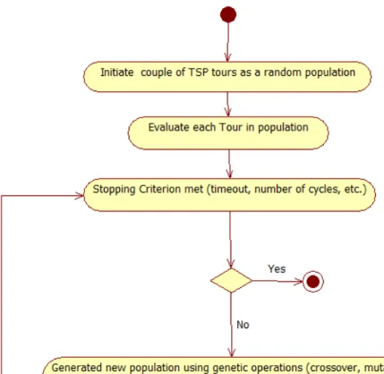
Figure 2 shows the simple structure of Genetic Algorithm. GA begins with random initiation of a population using chromosomes as abstract presentations of solution candidates. Chromosomes encode feasible. The population evolves successively. A portion of population, which is evaluated as better individuals, is chosen for breeding. The selecting process is based on a fitness function, which delivers the fitness of each individual. The "breeding" or so-called "reproduction" step of GA is applying natural genetic operators such as Selection, Crossover, and Mutation for each two chosen individuals. The new child will share characteristics of its parents. The generational process will be stopped until the pre-defined criteria are met. The typical criteria can be the number of created generations, runtime of generation process, pre-defined level of fitness or the combination of all above mentioned criteria. Those criteria depend strongly on the real problem and real conditions, in which the resource like computational performance should be taken into consideration.

(22)

22

Figure 2: Simple Structure of Genetic Algorithm applied in TSP

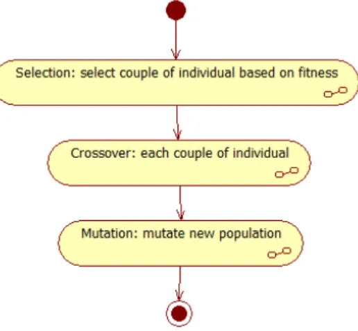
In the above structure of Genetic Algorithm, the Genetic Algorithm takes parameters as random set of TSP tours and a function to evaluate tour length. Every time it returns a new population, which is in TSP a new tour, the evaluation function is applied to each individual in the new population to calculate population’s average fitness and the fittest individual. Genetic Algorithm applied natural genetic operations and expects that the new generated population always better than the old one as the “survival of the fittest” rules the evolution. Figure 3 depicts 3 steps of generating new population.

3.2.2. Initiation a random population

The first step of GA is to initiate a new random population. Before doing that, it is necessary to define the population size. In TSP, the question is how many random tours should be created for the first population. Size of population can be constant or can vary after each evolution cycle. The stopping criterion of the algorithm also needs to be specified in this step. It can be a limitation of timing and/or population age. One typical problem of heuristic algorithm is when the algorithm should stop. Timing can be understood as the algorithms starts, and after a pre-specified time span, even that

(23)

23

population’s fitness is still improving, we need to stop the algorithm. Population age is number of generation cycles, in which population’s fitness does not improve. The best fitness in this case should be accepted as the best solution the algorithm can delivery.

Figure 3: Generating new population

3.2.3. Evaluation function

In TSP, it is easy to choose a fitness/evaluation function. The fitness function takes a tour as input parameter and return tour length for evaluation. Good individual will deliver high fitness; in TSP it means better tours have shorter travelling distance to the salesman. Evaluation result has a crucial role in choosing mating couples for generating next generations. Taking good individuals to create parents strengthens the hope that their offset in the next generation will have better fitness, or at least as strong as its parents. In some specific case, the best individual in a population remains in the next generation, because after crossover mutation the best individual can be lost.

3.2.4. Genetic Operations

Selection

Randomly two individuals are chosen for producing tentative offspring. The selection is based on fitness of individual. In TSP, shorter tours have greater possibility to be chosen. One good individual can take part in several mating processes; the number of its copies is directly proportional to its fitness. When a very good tour is found in TSP, it is used to produce some more similar good tours in next generation. This step mimics the natural procedure which is called proportional selection scheme [6].

(24)

24

Crossover

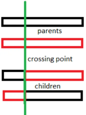
After choosing parents, next step will be how the parents get their offspring. That is where Crossover operation comes in play. The main role of crossover in the nature is to randomly select parts of a parent individual and combine them to create new offspring. There are several types of crossover, and the most common type is single point crossover. Single point crossover chooses a location of one parent chromosome, packs into child chromosome and the rest of this child chromosome is copied from another parent. Figure 4: single point crossover shows us there is only one point of crossover, that why the operation is called single point cross over. There are some possibilities which should be defined at this point such as possibility for the happening of crossover because it can happen that the parent can not cross each other at all but just copy themselves directly to their child. Possibility for deciding whether only one offspring or two should also be defined by implementing this algorithm.

Figure 4: single point crossover

Many combinational problems can be used one point cross over, because they can present their solution candidates in a binary form. But in TSP it is quite difficult to do that. Solution candidates in TSP are sequences of paths between cities, like the followings:

• parentTour1 = [1 2 3 4 5 6 7 8 9 10]

• parentTour2 = [3 6 8 9 2 5 1 4 7 10]

Application of one point crossover is not appropriate in this case. Assumed that we choose the fifth cities as the crossing point, the child tour looks like:

(25)

25

• childTour = [1 2 3 4 5 5 6 4 7 10]

The childTour violates TSP’s rule of visiting each city only once as city 8 does not exits in this tour.

There is another approach of Crossover in TSP, actually named Cycle Crossover

(Karova, Smarkov, & Penev, 2005). In Cycle Crossover, cities are taken from each parent and put into their child at the exact locations like them in the parent. For example, city 1 is taken from parent 1; city 10 is taken from parent 2:

• childTour1&2 = [1 - - - -]

Because the first position is occupied by city 1 of parent 1, city 3 of parent 2 cannot be there, that means city 3 have to be taken from parent 1, again.

• childTour1&2 = [1 - 3 - - - -] Keep doing that, we have:

• childTour1&2 = [1 - 3 4 - - 7 8 9 -]

All cities in the above tour is taken from parent 1, we fill it up with other cities in parent 2:

• childTour1&2 = [1 6 3 4 2 5 7 8 9 10]

This Cycle Crossover approach helps us exchange cities to visit randomly, but does not guarantee that the numbers of cities taken from both parents are fairly equal. An example:

• parentTour1 = [1 2 3 4 5 6 7 8 9 10]

• parentTour3 = [10 1 2 3 4 5 6 7 8 9]

Apply the same Cycle Crossover as mentioned, we have the child tour exactly identical to parentTour1: childTour1&3 = [1 2 3 4 5 6 7 8 9 10]. If this happens, crossover is stuck on this specific tour. This is for the time mutation operation coming in play.

Mutation:

Selection and Crossover are processed rapidly until a new full population comes out. Because it is possible that all the new individuals are exact the same like in the older

(26)

26

population. A mutation operation on all new individuals can guarantee that will not happen. A loop through the population, and change at one encoded position is applied to each individual. Mutation guarantees that the algorithm is not trapped into one local or sub-optimal solution.

An example of Mutation in TSP:

• Tour = [1 6 3 4 2 5 7 8 9 10] before apply Mutation.

• Tour = [1 9 3 4 2 5 7 8 6 10] after apply Mutation to position 2 and 9

3.3.Ant-Colony Optimization

Recently many algorithms have been inspired by mimic and simulating the natural behavior of a real ant in its community to solve difficult discrete optimization problems. The word “Ant System” (AS) was the first time mentioned in [7]. In this paper, Dorigo and his colleges have defined an Ant System algorithm derived from behaviors of artificial ant colonies. To test diverse branches of the algorithms as well as finding the optimal parameters, they applied the algorithms to Travelling Salesman Problem. In 1996, Dorigo and his colleagues introduced an improvement of Ant System algorithm and named it Ant-Colony System (ACS) in the paper titled “Ant Colony System: A Cooperative Learning Approach to the Traveling Salesman Problem” [8]. ACS is a crucial improvement of AS because it can solve large TSPs much more effectively than AS.

3.3.1. Biological Background

In reality, a natural ant colony consists of millions of individuals. In an ant community, there are different kinds of ants which have different tasks and responsibilities: worker, soldiers and thequeen. One of ant-worker’s (or –agent’s) tasks is to find the food source and bring food back to their colony. Although an ant is blind, it is found that ants mostly find the shortest way from colony to source food. Once the path is found, ants communicate with each other through a special communication media: the pheromone. Pheromone is the chemical substance ants lay on their path in finding food. The intensity of pheromone-trail has the most important role in ant moving direction. The Ant nest can be considered as a start position for all ants for searching for food. Assumedly there is only one food source and there are many distinguish ways from the

(27)

27

colony to the source. Each way has its own distance and if all ants move at the same speed, it means the shortest way takes the shortest travel time from colony to the food source.

3.3.2. Ant System

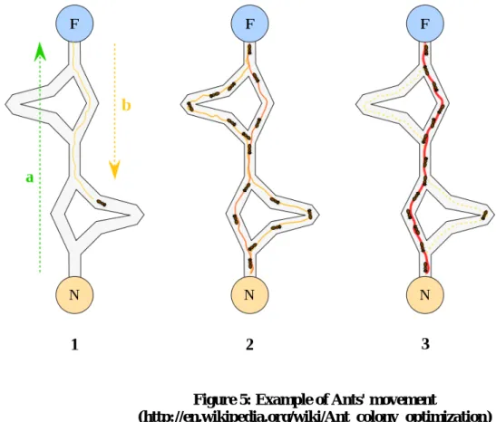
The problem finding food of ants can be presented by a graph G = (V, E). V is the set of nodes in the Graph, and E is an edge between two nodes. In TSP, each vertex v in V can be seen as a city and E is the road between two cities. As above mentioned, ants deposit pheromone and they cooperate with each other through the intensity of pheromone trail. The main parts of the algorithm are the movement decisions of an ant from one node to another, local pheromone updating in each edge when an ant walks in the edge and the global pheromone updating which updates all the edge an ant has visited before completes the tour.

Figure 5: Example of Ants' movement

The crucial factors in ants’ moving decision are the town distance and the amount of trail present on the connecting edge [7].

(28)

28

Following is the definition of the transition probability from city i to city j of Ant System algorithm:

pij(t) = �

[𝜏𝜏𝑖𝑖𝑖𝑖(𝑡𝑡)]𝛼𝛼.�𝜂𝜂𝑖𝑖𝑖𝑖�𝛽𝛽

∑[𝜏𝜏𝑖𝑖𝑖𝑖(𝑡𝑡)]𝛼𝛼.�𝜂𝜂𝑖𝑖𝑖𝑖�𝛽𝛽 𝑖𝑖𝑖𝑖𝑖𝑖 ∈ 𝒂𝒂𝒂𝒂𝒂𝒂𝒂𝒂𝒂𝒂𝒂𝒂𝒂𝒂

0 𝑜𝑜𝑡𝑡ℎ𝑒𝑒𝑒𝑒𝑒𝑒𝑖𝑖𝑒𝑒𝑒𝑒

This formula is taken from [7] when they apply the algorithm to TSP. η_ij is the visibility of the road from i to j, which is disproportional to the distance from i to j: η_ij = 1/dij.

τij(t) is the density of pheromone on the road from i to j. α und β are parameter for controlling the relative importance of trail versus visibility. If β is much greater than α,

which means the distance have a great importance; the algorithm tends towards to the Greedy Algorithm.

After complete a tour, each ant compares his tour with the best global tour and update it if it has just travelled through a better tour, which in this case a tour with less cost. There are 3 models of ant algorithms: Ant-Density, Ant-Quantity and Ant Cycle. They differ from each other by how and when ants and ant-colony update pheromone. ∆τ_ijk is the amount of pheromone an ant puts on a road between i and j.

Ant-Density Model: ∆τ_ijk = � Q if the k−ant go through the i−j path 0 otherwise Ant-Quantity Model:∆τ_ijk = �

Q

dij if the k−ant go through the i−j path

0 otherwise Ant-Cycle Model:∆τ_ijk = �

Q

Lk if the k−ant go through the i−j path

0 otherwise With Lk being the total tour distance of the k-ant

(29)

29

According to [9] cycle model is not as near to the reality as density and Ant-quantity. But for the optimization purpose, Ant-cycle has great advantages against other two models. In Ant-cycle model, only the “good” tours are taken to update global pheromone. Experiments have showed that applying Ant-cycle into TSP brought a very good result in compare with other models. Thus, Ant-cycle model will be applied to solve STCP.

3.3.3. Ant Colony System

Ant Colony System (ACS) is an improvement of Ant System. ACS was mentioned for the first time in [8] when authors tried to improve efficiency of Ant System for solving symmetric and asymmetric TSP. Their experiments say that the Ant System Algorithm can discover good tours up to 30 cities, but requires much more time for larger problems.

ACS is basically based on AS. Main differences lay on aspects of how pheromone trail updated, transition decision of ants and how ants locally communicate with each other.

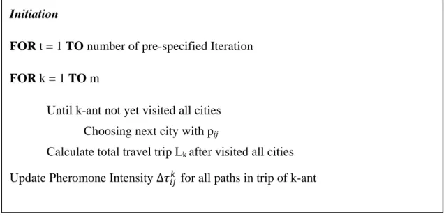
Initiation

FOR t = 1 TO number of pre-specified Iteration FOR k = 1 TO m

Until k-ant not yet visited all cities Choosing next city with pij

Calculate total travel trip Lk after visited all cities Update Pheromone Intensity ∆𝜏𝜏_{𝑖𝑖𝑖𝑖}𝑘𝑘 for all paths in trip of k-ant

(30)

30

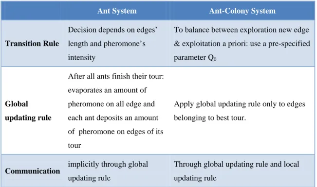
The following table describes the differences of these two algorithms in 3 aspects:

Ant System Ant-Colony System

Transition Rule

Decision depends on edges’ length and pheromone’s intensity

To balance between exploration new edge & exploitation a priori: use a pre-specified parameter Q0

Global updating rule

After all ants finish their tour: evaporates an amount of pheromone on all edge and each ant deposits an amount of pheromone on edges of its tour

Apply global updating rule only to edges belonging to best tour.

Communication implicitly through global

updating rule

Through global updating rule and local updating rule

Table 3: Compare Ant System and Ant-Colony System

State Transition Rule of ACS can be described with the formula:

𝑒𝑒= � 𝑎𝑎𝑒𝑒𝑎𝑎 𝑚𝑚𝑎𝑎𝑚𝑚⁡{[𝜏𝜏(𝑒𝑒,𝑢𝑢)].�𝜂𝜂(𝑒𝑒,𝑢𝑢)]𝛽𝛽� if q<q0(exploitation)

𝑒𝑒𝑎𝑎𝑟𝑟𝑟𝑟𝑜𝑜𝑚𝑚𝑟𝑟𝑟𝑟𝑒𝑒𝑒𝑒𝑟𝑟𝑒𝑒𝑐𝑐𝑡𝑡𝑟𝑟𝑒𝑒𝑚𝑚𝑡𝑡𝑟𝑟𝑜𝑜𝑟𝑟𝑒𝑒 otherwise (exploration)

s is the next node to visit with an ant located at node r. Q0 is a pre-specified parameter impacting the decision between exploitation or exploration, 0≤Q 0 ≤1. q is a random variable created every times an ant calls transition rule.

The crucial difference between AS and ACS lays on the global updating rule. Only the ant, which makes globally best tour, is allowed to deposit pheromone on his path. With this rule, in next iterations of the algorithms, ants will search around the last best tour. Local Updating Rule is a branch-new operation of ACS. With this rule, ants are allowed to change pheromone level of the edges when they visit. According to (Dorigo & Gambardella, 1996), the Local Updating Rule has the purpose to shuffle the tour. It avoids ants to be stuck around the sub-optimal tours. Compared to the Genetic Algorithm’s permutation operation, this rule has the same goal.

(31)

31

Chapter 4 Implementation a test bench for

STCP

The test bench for performance comparison between algorithms applied in STCP is implemented in object-oriented methodology using Java and Eclipse IDE. Programming framework for Ant Colony Algorithm is the “Java for Ant-Colony Systems Framework” [10] and a framework for Genetic Algorithm is “Java Genetic Algorithm Solution” [11].

4.1.Test Bench Structure

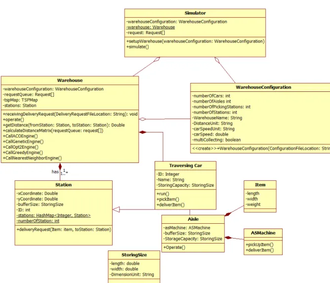
The test bench has 4 main packages: warehouse, TSP, simulation and Algorithms. The warehouse package contains all classes abstracting the simple warehouse model used to interpret the Sequencing Traversing Car in a Warehouse Problem. TSP package abstracts Travelling Salesman Problem in classes: City, TSPMap, and Salesman. Simulation package contains a Simulator class, which provides methods to generate test cases, report comparison result, setup and run the warehouse model. The Algorithm package contains classes of for TSP applied algorithms.

There is a class named WarehouseConfiguration in the warehouse package including all information of a warehouse instance which is number of cars, aisles, picking stations speed and of the traversing car. A warehouse instance has an array of order and an array of station. Methods for finding optimal tour for a set of orders are defined and named like: CallACOEngine, CallGeneticEngine, CallGreedyEngine, etc. These methods then create corresponding algorithms, passing parameters and receive back the most optimal tour that the algorithms can find. Stations are identified with ID and XCoordinate, YCoordinate. There are in fact 3 types of stations: aisle, input/output point and picking station, but in this warehouse model, we assume that the buffer size is defined as unlimited; hence it is no difference between three types of stations.

(32)

32

One of the most important parts of solving STCP is to transforming it in to TSP problem, which in this case asymmetric TSP. To do that, we import warehouse configuration, picking order request and from that information, we generate a distance matrix. The matrix is calculated based on stations’ location and orders’ information. As mentioned in 2.6, STCP can only be transformed to asymmetrical TSP or generalized TSP which takes only setup information as a matrix of distance between cities.

Figure 7: STCP test bench’s main class diagram

Input file format for STCP workbench is in XML-format. The Configuration XML contains information corresponding to WarehouseConfiguration’s attribute. The Order XML has a list of orders, with order ID, start and destination of each order. The workbench use Dom4J framework to read XML file and parse XML with XPath. Following is an example of Order XML

(33)

33

Figure 8: a sample of XML order file

Figure 9: Parsing XML configuration file with XPath using Dom4J Framework

4.2.Frameworks

This section introduces programming frameworks and libraries used in construct the test bench.

@SuppressWarnings({ "unchecked" })

public void ReceivingDeliveryRequest(String RequestFileLocation)

throws DocumentException {

File ConfigurationFile = new File(RequestFileLocation); SAXReader xmlReader = new SAXReader();

Document requestDoc = xmlReader.read(ConfigurationFile); List<Node> requestNodes =

List<Node>)requestDoc.selectNodes("//Request");

int numberOfRequest = requestNodes.size();

requestQueue = new Request[numberOfRequest];

//System.out.println(requestNodes.get(0).selectSingleNode("From").get Text());

for (int i = 0; i < numberOfRequest; i++) {

int from =

Integer.parseInt(requestNodes.get(i).selectSingleNode("From").getText ());

int to =

Integer.parseInt(requestNodes.get(i).selectSingleNode("To").getText() );

int ID = Integer.parseInt(requestNodes.get(i).valueOf("@ID"));

…

<?xml version="1.0" encoding="UTF-8"?> <DeliveryRequest>

<Comment>a sample of request file for traversing car</Comment> <Date>10/02/2010</Date> <Time>07:00</Time> <Request ID="01"> <From>4</From> <To>6</To> </Request> <Request ID="02"> <From>3</From>

(34)

34

4.2.1. Java for Ant-Colony Systems Framework (JACSF)

JACSF is chosen as a framework to solve STCP in this thesis, because it is one of the closest implementations to Ant-Colony System described in [8] of among others programming libraries. And JACSF was also implemented to solve generalized TSP, meanwhile other implementations like Concorde restricted to solve only symmetric TSP.

JACSF is an Object-Oriented framework written in Java designed by Ugo Chirigo [10] to implement Ant Colony System. This framework is chosen for testing the efficiency of Ant Colony System in solving Sequencing Traversing Car in a Warehouse Problem. JACSF has implemented the idea of Dorigo and Gambardella of Ant Colony System in [8]. The Ant Colony System is described in 3.3.3 of this thesis. Three important aspects of Ant Colony System implemented in JACSF are:

“

• a State Transition Rule which brings the concrete ant from a node to another across an arc;

• a Local Updating Rule which updates the pheromones deposited by the ant on the arc it walked in;

• a Global Updating Rule which updates the pheromones deposited on the arcs when an ant ends its tour;

“

JACSF has 3 main entities: Ant, AntColony and a AntGraph. An Ant Colony System contains a set of ants, a graph and an ant colony, which plays the global updating job of the algorithm. Figure 10: Object Model of JACSF in UML depicts these entities in UML.

The object model of JACSF has two abstract classes: Ant and AntColony. Ant implements behavior of an artificial ant which, during the searching process, has to make transition decision and update local pheromone trail. These two methods are abstracts and implemented in the context of specific problem. AntColony is an abstract class implementing the Ant Colony System. Two methods need to be implemented in derived classes are creatAnt and globalUpdatingRule. AntGraph class contains information of pheromone density and distance between nodes in graph.

(35)

35

To apply JACSF to TSP, the transition rule, global updating rule and local updating rule should be implemented in two derived classes of Ant and AntColony. Formula of those rules is described in 3.3. The path in STCP differs than in TSP that it does include distance from last visited city to the city where the salesman starts.

4.2.2. Genetic Algorithm Framework

As mentioned, the Genetic Algorithm Framework used for performance testing is Java Genetic Algorithm Solution (JGAS) [11]. This framework is chosen because it contains not only Genetic Algorithm’s implementation but also others optimization algorithms like 2-opt, Greedy Algorithm. Like JACSF, Java Genetic Algorithm Solution also uses the power of parallel programming to speed up algorithms’ runtime and can solve a TSP with up to 5000 cities. This framework also accepts a TSP defined with a distance matrix between cities. Thus, it is capable to solve generalized TSP, especially asymmetrical Travelling Salesman Problem. Supported algorithms by JGAS are:

• Random Mutation: simply mutate two random tour with each other

• JGAP Genetic Algorithm: implementation of an open-source java genetic framework

• Genetic Algorithm: Genetic Algorithm with crossover and mutation operations

(36)

36

• Genetic Algorithm with 2-opt optimization: a very fast solution of TSP using GA and 2-opt (Sengoku & Yoshihara, 1998)

• 2-opt optimization: implementation a pure 2-opt optimization. The optimization is based on random mutation.

4.2.3. TSPLIB

TSPLIB is not a framework; it is a library of test instance for TSP and TSP-related problems. TSPLIB is used to benchmark solutions. The benchmark instances are given with varying complexity and difficulty. STCP is considered in this thesis as a related problem to TSP.

The TSPLIB format has two parts: specification part and a data part. In the specification part all entries are in the form <keyword> : <value>. The specification parts contain the configuration of the TSP like: name, type of TSP (asymmetric, symmetric), edge weight format (given in function of matrix format), etc. The data part of TSPLIB files has the format depending on the choice of the specification. Each section of data part begins with a corresponding keyword and the information begins with a new line. End of data part is defined in the specification section. More details of can be found in [12].

The STCP Test bench provides a module to translate XML input file to TSPLIB format file as an Asymmetrical Travelling Salesman Problem. With this standard format for TSP, STCP can be solved directly by programs which accept TSPLIB file format.

4.3.Testbench workflows

Figure 11: xml – to - tsplib workflow and Figure 12: xml - to - distance matrix workflow present two possible workflows of the test bench. In the first workflow, STCP configuration file and delivery order files are transformed directly to TSBLIB file then use solutions, which take TSPLIB format as input, to solve STCP. In the second workflow, configuration file and delivery order file is translated to a matrix of distance, then use framework of genetic and ant colony system to solve that asymmetric matrix. Because the configurations file as well as delivery order file is in XML-format, the first workflow is called TSPLIB and the second workflow is called XML-to-DistanceMatrix.

(37)

37

4.2.4. Setup warehouse:

The test bench takes at least two files before asking a warehouse model to execute a set of orders. One of them is a configuration file for setting up warehouse model, and the other is the order file in XML format. A configuration file contains information of the warehouse, which indicates where the stations are and how far they are from each others, is similar to specify the city coordinate in TSP and their distance to other city. The setup process begins with a simulator instance call method setupWarehouse with parameter as a String referring to setup file location.

Figure 11: xml – to - tsplib workflow

(38)

38

4.3.1. Delivery Orders:

After the warehouse is configured, it is ready to take delivery orders. Delivery orders are specified in a XML file. Simulator decides which set of orders should be executed. After locating the information of picking orders, the warehouse instance will create a TSPLIB format file or a two-dimensional distance matrix.

4.3.2. Calculating Best Tour:

The warehouse instance sends a matrix of distance to solutions engines, which is based on routing algorithms like Genetic Algorithms or Ant-Colony System. It also deliver pre-specified parameter for each solution engines. For example in Genetic Algorithm, that is the population size, in Ant-Colony System, that is the number of ants. After solutions engines finishing their computation, they return the best tour back to the warehouse, which forwards the results further to the simulator instance. Because the warehouse model built is just for comparison between algorithms, the workflow should stop here. In reality, after comparing results of solutions engines with each others, the warehouse will instruct a traversing car to execute a sequence of picking orders.

4.3.3. 55BIntegrating other algorithms

There are two situations possible for plugging other algorithms into this test bench. First variant is the algorithms are already used to solve TSP. That means it should be able to take a distance matrix as a parameter and calculation of tour length as evaluation function. In this case, we only need to implement an adapter class for the new algorithm The adapter class must have the function findBestTour(double[] distanceMatrix). In the other case, the new heuristic algorithm has not been applied to TSP yet. Because it is a heuristic algorithm, we need to define encoding function and evaluation. This test bench is designed to use algorithms which have been already coded to solve TSP.

(39)

39

Chapter 5

7B

Performance Comparison of

Algorithms to STCP

In this chapter we also compare performance of several algorithms applied in STCP. The comparison result is basis for the suggestion of using which algorithms in which case of STCP. One of the main tasks of chapter 5 is to define test cases for tuning Ant-Colony System Algorithm and Genetic Algorithm to get optimal configurations of two algorithms when apply them to Sequencing Traversing Car in a Warehouse Problem.

5.1.27BSetup Test Bench

For tuning configuration of Ant-Algorithm and Genetic Algorithm, there is a set of 50 delivery orders in a 4 aisle, 4 picking station, 1 input point and 1 output point. Location of stations is specified with 2-Dimension coordinate system. Measure unit of coordination system is meter. Speed of the traversing car is 2 m/s, single-collecting car. Followings are station coordination:

• Input Point: < 0, 0 > • Output Pont: <25, 0> • Aisle 1: < 50, 0 > • Aisle 2: < 75, 0 > • Aisle 3: < 100, 0> • Aisle 4: < 125, 0> • Picking station 1: < 50, 0 > • Picking station 2: < 80, 0 > • Picking station 3: < 110, 0 > • Picking station 4: < 140, 0>

(40)

40

For algorithm tuning we use only one set of 50 delivery orders. To compare algorithms’ performances with each other, we have several sets of delivery order which contain from 50 up to 2000 orders.

Because there is no exact solution implemented, a set of order with a tour which has a total un-loaded travel time is 0 meter as the optimal tour. With this set of order, we can analyze how low it takes an algorithm to reach to the optimal tour.

5.2.28BTuning Ant-Colony Algorithm applied to STCP: Number of ants

In order to achieve optimal number of ants for a set of 50 orders, a test is launched with fix factors: β = 2, α = ρ = 0.1, max number of cycle is 2500 and Q0 is 0.8. For each number of ants, at least 10 tests are executed.

Number of Ants

Un-loaded distance of the best found tour

Average un-loaded distance for 10 tests

Average number of cycles before entering best Uni-path.

10 305 meter 322 meter 911

20 320 meter 322 meter 876

30 305 meter 315,5 meter 721

Table 4: Tuning number of Ants in Ant-Colony Algorithm

Table 4 reveals a minor difference of best tours as well as the average of best tour distance in 10 tests corresponding to the number of ants. As in Table 4, the more ants there are the faster we get into the best Uni-Path. It can be explained that when we have more ants on the map, the intensity of pheromone trail is stronger in all paths, especially the shortest path and some near-shortest paths. Best tours showed in the table can possibly be the optimal global tours, or just sub-optimal tours which ants are stuck in. With a decision factor Q0 = 0.8 (80% exploitation, 20% exploration) and max number of iteration is 2500, colony setup with 20 ants like in the above table seems like cannot find the tour with un-loaded travel distance of 305 meter.

We have experimented runtime of Ant-Colony System with increasing number of ants, and result is in Diagram 1. The graph captures the growth of running time of ACS with a set of 50 picking orders. It shows us that the algorithm runtime rises linearly. Take it as an indicator for choosing number of Ants for a set of 50 orders, we will set number of ants at 10 as suggested in [8].

(41)

41

Diagram 1: Runtime of Ant-Colony Algorithm with increasing number of ants

5.3.29BTuning Genetic Algorithm applied to STCP

As mention in 3.2, two parameters of Genetic Algorithm should be tuned in order to attain the best configuration for the algorithm is population size, permutation rate. We apply the same set of 50 delivery orders like in tuning ASC. Permutation rate is fixed at 10%. The stopping criterion for GA is population age equaling 100, which means the algorithm stop by 100 cycles. Criteria used to choose the number of population is algorithm’s runtime and tour distances it delivers. Following is the tuning result of population size:

Diagram 2: Tuning population size of GA for a set of 50 orders

0 50 100 150 200 250 1 5 9 ₁₃ ₁₇ ₂₁ ₂₅ ₂₉ ₃₃ ₃₇ ₄₁ ₄₅ ₄₉ ₅₃ ₅₇ ₆₁ ₆₅ ₆₉ ₇₃ ₇₇ ₈₁ ₈₅ ₈₉ ₉₃ ₉₇ (s) Number of Ants 0,00 0,50 1,00 1,50 2,00 2,50 3,00 3,50 4,00 4,50 5,00 0 100 200 300 400 500 600 700 800 10 40 70 ₁₀₀ ₁₃₀ ₁₆₀ ₁₉₀ ₂₂₀ ₂₅₀ ₂₈₀ ₃₁₀ ₃₄₀ ₃₇₀ ₄₀₀ ₄₃₀ ₄₆₀ ₄₉₀ ₅₂₀ ₅₅₀ ₅₈₀ ₆₁₀ ₆₄₀ ₆₇₀ ₇₀₀ ₇₃₀ ₇₆₀ ₇₉₀ ₈₂₀ ₈₅₀ ₈₈₀ ₉₁₀ ₉₄₀ ₉₇₀ 1000 se con d m eter size of population

(42)

42

Genetic Algorithm constantly delivers very good tour when population size is greater than 130. The graph also shows that GA’s computation cost for a set of 50 picking requests rises linearly to number of population size. In conclusion, from this experiment we can take population size of 150 for a set of 50 delivery orders to guarantee that GA delivers good tour in acceptable time.

Next tuning is about the Mutation Ration. Population size is set at 150, a set of Mutation Ration to evaluate is: {0; 0.1; 0.2; 0.3; 0.4; 0.5; 0.6; 0.7; 0.8; 0.9; 1}. Statistics are calculated across 10 trials. After experiments, we recognize very slight difference of GA runtime again increasing mutation ration. Thus AG’s runtime in this case is one factor that is not necessary to consider. The only remain interesting factor is the best average tour GA delivers with different value of mutation ration. Following charts depicts the experiments result:

Diagram 3: average unloaded-travel distance against mutation ration

Interestingly, with mutation ration from 0.5 to 0.7, GA returns the best tour of 305 meter across all 10 trials for each value. From the chart we can see that the average unloaded-travel time is extremely high with small value of mutation ration (up to 0.3). This can be explained that with small value of mutation rotation, GA is usually stuck into sub-optimal solutions. The value is too small to shuffle individuals, and then it is difficult to get to the most optimal tour. With higher value of mutation ration, GA also cannot deliver the best optimal tour, because it shuffles almost all individuals in the population, even the fittest. Thus, GA loses the fittest because of mutation and creates new weaker individuals. We choose 0.6 as the most optimal mutation ration in this circumstance. 290 295 300 305 310 315 320 325 330 335 0 0,1 0,2 0,3 0,4 0,5 0,6 0,7 0,8 0,9 1 m eter Mutation Ration

(43)

43

5.4.30BBenchmarking algorithms applied in STCP

In the last sections, we have tested and found the best optimal configurations for Ant-Colony System and Genetic Algorithms. In this section we benchmark algorithms with each other to see of how fast they can solve STCP, how good algorithms solve the problem, how scalar the algorithms are when rapidly increasing number of requests. The ultimate goal of benchmarking is to find the best algorithm in aspects of speed and quality of orders’ execution in STCP.

Algorithms in the benchmark are: Ant-Colony System, Genetic Algorithm, 2-opt Algorithm, Genetic-hybrid-2-opt Algorithm, Greedy Algorithm and FIFO approach. The first evaluation is about solution quality the algorithms can deliver. We test all algorithms with sets of {50, 100, 150, 200, 250, 300, 350, 400, 500} requests. Algorithms are tested across 10 trials. Following is the result:

Set of orders ACS Genetic Algorithm 2-opt Genetic-Hibrid-2opt Greedy FIFO Best found Avr. Best found Avr. Best found Avr. Best found Avr. 50 orders 320 326,5 305 307 355 368 355 367 475 2535 150 orders 855 902,22 665 683 765 782 745 765 900 6930

Table 5: Compare unloaded travel distances rendered by solution engines

The table shows us that in almost all cases, genetic algorithm always gets the best solutions. GA is convincingly good with every sets of picking orders. 2-opt algorithm has been proved to be a very effective approach to solve symmetric TSP, but through this table, we can see that it has the worst performance compare with all heuristic algorithms. It can be explained that 2-opt is only effective in a symmetric TSP, when it shorten crossed edges. In contrast to symmetric TSP, in TSP, unfold crossed edges can even makes a worse tour than a crossed one. Genetic Algorithms has brought a very