SFB 649 Discussion Paper 2006-072
Optimal Interest Rate
Stabilization in a Basic
Sticky-Price Model
Matthias Paustian*
Christian Stoltenberg**
* Bowling Green State University, Department of Economics, Bowling Green, USA
** Department of Economics, Humboldt-Universität zu Berlin, Germany
This research was supported by the Deutsche
Forschungsgemeinschaft through the SFB 649 "Economic Risk". http://sfb649.wiwi.hu-berlin.de ISSN 1860-5664
S
FB
6
4
9
E
C
O
N
O
M
I
C
R
I
S
K
B
E
R
L
I
N
Optimal Interest Rate Stabilization in a
Basic Sticky-Price Model
∗
Matthias Paustian,
†Christian Stoltenberg
‡September 2006
Abstract
This paper studies optimal monetary policy with the nominal interest rate as the single policy instrument in an economy, where firms set prices in a stag-gered way without indexation and real money balances contribute separately to households’ utility. The optimal deterministic steady state under commitment is the Friedman rule – even if the importance assigned to the utility of money is small relative to consumption and leisure. We approximate the model around the optimal steady state as the long-run policy target. Optimal monetary policy is characterized by stabilization of the nominal interest rate instead of inflation stabilization as the predominant principle.
JEL classification: E32, E52, E58.
Keywords: Optimal monetary policy, commitment, timeless perspective, optimal steady state, staggered price setting, monetary friction, Friedman’s rule.
∗We are especially thankful to Tim Fuerst, Harald Uhlig, Juergen von Hagen and Andreas Schabert.
Further, we would like to thank Dirk Kr¨uger, Michael Burda, Marco Airaudo and Mirko Wiederholt for suggestions and comments. This research was supported by the Deutsche Forschungsgemeinschaft through the SFB 649 “Economic Risk”. Earlier versions of this paper circulated under the title “The Inactiveness of Central Banks: An Issue of Optimality?”.
†Bowling Green State University, Department of Economics, Bowling Green, OH 43403, USA,
email: [email protected], fax: +1 419 372-1557, tel: +1 419 372-3491.
‡Humboldt University Berlin, Department of Economics, D-10178 Berlin, Germany, email:
1
Introduction
What is the primary aim of optimal monetary policy? In the existing literature there are two major views that deliver opposite recommendations for the optimal conduct of monetary policy in the short and in the long run. The first branch goes back to Friedman (1969) and evaluates monetary policy in the long run with fully flexible prices and under perfect competition. In order to equate the private opportunity costs for holding money to the zero social costs to produce it, the nominal interest rate should be zero. The other view considers optimal monetary policy in the short run in the presence of nominal rigidities and imperfect competition (e.g. Woodford, 2003a, ch.6-8; Benigno and Woodford, 2005; Khan et al., 2003; Schmitt-Groh´e and Uribe, 2004, 2005). A key feature of this literature is that the authors consider small fluctuations around the (almost) zero inflation steady state, implying that optimal policy nearly completely offsets the distortions due to price dispersion – even in the presence of a monetary friction. The predominant principle is inflation stabilization, while the nominal interest rate should adjust relatively freely to support this principle (Woodford, 2003a).
In this paper we revisit the issue of optimal monetary policy in a sticky price model in the presence of a transaction friction. The foremost contribution is to challenge the conventional view that the Friedman rule loses out to the goal of price stability once price stickiness is introduced. We show that the widely used money-in-the utility function model (MIU) implies that Friedman’s rule is optimal even when large amounts of price stickiness are present. This is in contrast to the key message of papers such as Woodford (2003a), Khan, King and Wolman (2003) and Schmitt-Groh´e and Uribe (2004, 2005) and others. Second, we find that the primary aim of optimal policy in the short run is to stabilize the nominal interest rate instead of inflation.
Our analysis is set in a dynamic stochastic general equilibrium model with imperfect competition and Calvo’s staggered price setting (1983) without indexation. A
trans-action friction is introduced via the textbook money-in-the-utility-function approach (Sidrauski, 1967; Woodford, 2003a; Walsh, 2003) with consumption and real money balances entering in a separable way. Assuming that the government has access to lump-sum taxes, we focus on optimal monetary policy that relies on the risk-free nom-inal interest rate as the single policy instrument. Since we allow for the existence of an output subsidy that offsets the distortion created by monopolistic competition, the pol-icy maker faces two distortions: price dispersion due to staggered price setting calls for an optimal inflation of zero, implying costs of money holdings. However, the monetary distortion can only be offset by setting the nominal interest rate to zero.
We determine the optimal deterministic steady state under commitment as the optimal long-run target of monetary policy.1 Remarkably, we find that even for very
low values for the weight of money in the utility function relative to consumption and leisure, it is optimal to fully offset the monetary distortion and to allow for a small degree of price dispersion. I.e. the Friedman rule is optimal even in the presence of Calvo-style staggered price setting. This result holds for wide a range of parameter values including low weights for real money balances in the utility function. To understand this finding, note that the welfare cost of price dispersion arising from long-run deflation required by the Friedman rule is small relative to the loss from a positive nominal interest rate. While the welfare loss due to price dispersion hinges primarily on the frequency of price adjustment, the utility losses of a positive interest rate crucially depends on the sensitivity of money demand to the nominal interest rate. In an MIU framework, the latter increases strongly as interest rates fall. Thereby, the taxation of money holdings via a positive interest rate becomes suboptimal.
We linearize the model around the optimal steady state under commitment as the long-run optimal policy target and derive a quadratic approximation to the utility of 1To be more precise, we consider policies that are optimal from a timeless perspective (Woodford,
the representative household as the objective of the central bank. This welfare based loss-function depends on three arguments: the unconditional variances of inflation, the output gap, and on the variance of the nominal interest rate. While the weight for the variation in the output gap relative to inflation depends exclusively on deep parameters, the relative weight for interest rate variability hinges on steady state values, too. Re-markably, the preference to stabilize fluctuations in the nominal interest rate increases as optimal inflation moves towards Friedman’s rule of deflation. This increase is pri-marily driven by the rise in the interest elasticity of money demand. Correspondingly, the importance to account for monetary frictions depends upon the steady state chosen for approximation: The long-run optimal policy is key for optimal policy reactions in the short run. Since we approximate our model around a steady state implied by the Friedman rule, the primary goal of optimal monetary policy is to stabilize variations in the interest rate rather than in inflation. Given the high weight attached to interest rate stabilization, optimal monetary policy requires abstaining from fluctuations in the nominal interest rate. Instead, the nominal interest rate is literally fixed in response to various kinds of disturbances. In that sense, the observation that central banks keep the main refinancing rate constant over a long time horizon, e.g. the European Central Bank from June until December 2005, can be interpreted as optimal policy according to Friedman’s rule – even if the state of the economy has changed.
We show that choosing a long-run deflation target according to the Friedman rule does not generally undermine the central banks ability to stabilize the welfare rele-vant fluctuations around that target. On the contrary, the welfare loss arising from fluctuations around the Friedman steady state can be lower than the loss arising from fluctuations around the zero inflation steady state. Overall, we find support for the Friedman rule even in case of a reasonable amount of nominal rigidity due to staggered price setting a la Calvo: The Friedman rule yields higher steady state utility and can
also improve welfare effects of fluctuations around the steady state compared to price stability.
Regarding the lower bound on the nominal interest rate, we find that this is not a concern for central banks in our model. We assume that the zero bound on interest rates is not binding in expectations, i.e. the average gross nominal interest rate must be at least slightly larger than unity. While this assumption does not exclude the possibility of an occasionally binding constraint, the probability for this to occur is virtually zero. The standard deviation of the nominal interest rate under optimal policy is so small relative to the buffer between the steady state nominal rate and unity, that the lower bound essentially never becomes binding.
Related Literature
We now turn to the related literature. Most closely related to our paper is the work by Woodford (2003a, Chapter 6-7; Woodford, 2003b) and Schmitt-Groh´e and Uribe (2005). Woodford also studies optimal monetary policy in a money-in-the-utility func-tion framework with staggered price setting. In contrast to our analysis, the model is log-linearized around the zero inflation steady state without computing the optimal steady state in a first step. This approximation point then implies very different dy-namics for the nominal interest rate. In his analysis, the nominal interest rate reacts rather sharply to shocks while the optimal path of inflation is relatively smooth over the cycle (see Woodford, 2003a: 504). Our contribution is to show that the optimal policy prescriptions differ substantially once one takes into account the interactions between long run and short run optimal policy.
Schmitt-Groh´e and Uribe (2005) and Khan et al. (2003) also analyze optimal mon-etary policy with nominal rigidities and a monmon-etary friction. These papers adopt a transaction technology approach to introducing money into the model. While Khan
(2003) use a different time dependent pricing model than we do, the economic envi-ronment of Schmitt-Groh´e and Uribe (2005) is more similar to our framework. They analyze a medium scale model with staggered price setting a la Calvo and various ad-ditional distortions. They find that the central bank should aim at price stability and stabilization of inflation as the main principle. The difference between their key finding and our results is explained as follows. The money-in-the-utility function approach we employ has different implications for money demand at low interest rates compared to the transactions technology in Schmitt-Groh´e and Uribe. The MIU framework implies that the interest-elasticity of money demand increases by large amounts as the nominal interest rate approaches the lower bound. Correspondingly, welfare costs of positive interest rates increase substantially. This is not the case for their transaction cost tech-nology. Our contribution is to show that both the degree of price dispersion, as well as the sensitivity of money demand with respect to nominal interest rates at low levels, are decisive for the conduct of optimal policy.
Methodologically, this paper differs from Khan et al. (2003) and Schmitt-Groh´e (2005) by working with the linear-quadratic framework, rather than with the time in-variant Ramsey approach. By showing that the weight on nominal interest stabilization in the loss function depends on the steady state values under control of the central bank, this approach helps to point out intuitively how long run optimal policy and short run stabilization policies are interrelated. In addition, the guiding principle of optimal mon-etary policy is directly transparent in the size of the relative weights to stabilize the nominal interest rate, inflation, and the output gap.
The remainder of this paper proceeds as follows: in section 2 we set up the model. In section 3 we compute the optimal steady state under commitment and derive a quadratic approximation of the utility of the representative household. In section 4 we derive the optimal monetary policy responses in the short run for 2 policy regimes:
the first one has Friedman’s Rule, and the other one has zero inflation as its long-run target. The last section concludes.
2
The model
We consider an economy that consists of a continuum of infinitely lived households indexed with j ∈ [0,1]. It is assumed that households have identical initial asset endowments and identical preferences. Household j acts as a monopolistic supplier of labor services lj. Lower (upper) case letters denote real (nominal) variables. At the
beginning of periodt, households’ financial wealth comprises moneyMjt−1, a portfolio
of state contingent claims on other households yielding a (random) payment Zjt, and
one period nominally non-state contingent government bonds Bjt−1 carried over from
the previous period. Assuming complete financial markets let qt,t+1 denote the period
t price of one unit of currency in a particular state of period t+ 1 normalized by the probability of occurrence of that state, conditional on the information available in period t. Then, the price of a random payoff Zt+1 in period t+ 1 is given by Et[qt,t+1Zjt+1].
The budget constraint of the representative household reads
Mjt+Bjt+Et[qt,t+1Zjt+1]+Ptcjt ≤Rt−1Bjt−1+Mjt−1+Zjt+Ptwjtljt+
Z 1
0
Djitdi−PtTt,
(1) wherectdenotes a Dixit-Stiglitz aggregate of consumption with elasticity of substitution
θ, Pt the aggregate price level, wjt the real wage rate for labor services ljt of type j,
Tt a lump-sum tax, Rt the gross nominal interest rate on government bonds, and Dit
dividends of monopolistically competitive firms. Further, households have to fulfill the no-Ponzi game condition, limi→∞Etqt,t+i(Mjt+i +Bjt+i +Zjt+1+i)≥ 0. The objective
of the representative household is Et0 ∞ X t=t0 βt{u(c jt, ζt)−v(ljt) +z(Mjt/Pt)}, β ∈(0,1), (2)
where β denotes the subjective discount factor and Mjt/Pt = mjt end-of-period real
money balances. Note that our specification of utility is consistent with recent findings by Andr´es, L´opez-Salido and Vall´es (2006) for the Euro area and by Ireland (2004) for the US. They estimate the role of money for the business cycle of the Euro area and the US and find that preferences are separable between consumption and real money balances.
We assume that households’ utility can be affected by a disturbance term ζt with
mean 1 that can alter the utility of consumption. To avoid additional complexities, we set ucζ =uc at the deterministic steady state. For each value of ζ, the instantaneous
utility function is assumed to be non-decreasing in consumption and real balances, decreasing in labor time, strictly concave, twice continuously differentiable, and to fulfill the Inada conditions. We assume that z(mjt) implies satiation in real money
balances at a finite positive level. The derivativeszm, zmm have finite limiting values as
m approaches the satiation level from below. In particular, the limiting value of zmm
from below is negative (see Woodford, 2003a, Assumption 6.1).
Households are wage-setters supplying differentiated types of labor lj which are
transformed into aggregate laborlt with lt(²t−1)/²t =
R1
0 l
(²t−1)/²t
jt dj. We assume that the
elasticity of substitution between different types of labor,²t>1, varies exogenously over
time. The time variation in this markup parameter introduces a so called cost-push shock into the model that gives rise to a stabilization problem for the central bank. Cost minimization implies that the demand for differentiated labor services ljt, is given by
ljt = (wjt/wt)−²tlt, where the aggregate real wage ratewtis given byw1t−²t =
R1
0 w 1−²t
Maximizing (2) subject to (1) and the no-Ponzi game condition for given initial values Mt0−1 > 0, Z0, Bt0−1, and Rt0−1 ≥ 0 leads to the following first order conditions for consumption, money, the real wage rate for labor type j, government bonds, and contingent claims: λjt =uc(cjt, ζt), vl(ljt) = wjtλjt/µwt, (3) λjt−zm(mjt) =βEt λjt+1 πjt+1 , qt,t+1 = βλjt+1 πt+1λjt , λjt =βRtEt λjt+1 πt+1 (4)
where λjt denotes a Lagrange multiplier, πt the inflation rate πt =Pt/Pt−1, and µwt =
²t/(²t−1) the stochastic wage mark-up with mean ¯µw >1. The first order condition for
contingent claims holds for each state in periodt+1, and determines the price of one unit of currency for a particular state at timet+ 1 normalized by the conditional probability of occurrence of that state in units of currency in periodt. Arbitrage-freeness between government bonds and contingent claims requires Rt = 1/Etqt,t+1. The optimum is
further characterized by the budget constraint (1) holding with equality and by the transversality condition limi→∞Etβiλjt+i(Mjt+i+Bjt+i+Zjt+1+i)/Pjt+i = 0.
The final consumption good Yt is an aggregate of differentiated goods produced
by monopolistically competitive firms indexed with i ∈ [0,1] and defined as yθ−θ1
t =
R1
0 y
θ−1
θ
it di,withθ >1. LetPitandPtdenote the price of goodiset by firmiand the price
index for the final good. The demand for each differentiated good isyd
it = (Pit/Pt)−θyt, with P1−θ t = R1 0 P 1−θ
it di. A firm i produces good yi using a technology that is linear in
the labor bundle lit = [
R1 0 l (²t−1)/²t jit dj]²t/(²t−1): yit = atlit, where lt = R1 0 litdi and at is a
productivity shock with mean 1.
Labor demand satisfies: mcit =wt/at, wheremcit=mctdenotes real marginal costs
We allow for a nominal rigidity in form of a staggered price setting as developed by Calvo (1983). Each period firms may reset their prices with the probability 1−α independently of the time elapsed since the last price setting. The fractionα∈[0,1) of firms are assumed to keep their previous period’s prices, Pit =Pit−1, i.e. indexation is
absent. Firms are assumed to maximize their market value, which equals the expected sum of discounted dividends Et
P∞
T=tqt,TDiT, where Dit ≡Pityit(1−τ)−Ptmctyit and
we used that firms also have access to contingent claims. Here,τ denotes an exogenous sales tax introduced to offset the inefficiency of steady state output due to markup pricing (Rotemberg and Woodford, 1999). In each period a measure 1−αof randomly selected firms set new prices Peit as the solution to maxPeitEt
P∞
T=tαT−tqt,T(PeityiT(1−
τ)− PTmcTyiT), s.t. yiT = (Peit)−θPTθyT. The first order condition for the price of
re-optimizing producers is for α >0 given by
e Pit Pt = θ θ−1 Ft Kt , (5)
whereKt and Ft are given by the following expressions:
Ft=Et ∞ X T=t (αβ)T−tuc(cT, ζT(1))yT µ PT Pt ¶θ mcT (6) and Kt=Et ∞ X T=t (αβ)T−tu c(cT, ζT(1))(1−τ)yT µ PT Pt ¶θ−1 . (7)
Aggregate output is given by yt =lt/∆t, where ∆t =
R1
0(Pit/Pt)−θdi ≥ 1 and thus
∆t = (1−α)(Pet/Pt)−θ +απtθ∆t−1. The dispersion measure ∆t captures the welfare
decreasing effects of staggered price setting. If prices are flexible, α= 0, then the first order condition for the optimal price of the differentiated good reads: mct= (1−τ)θ−θ1.
the monetary authority is assumed to control the short-term interest rateRt. The fiscal
authority issues risk-free one period bonds, has to finance exogenous government expen-dituresPtGt, receives lump-sum taxes from households, transfers from the monetary
au-thority, and tax-income from an exogenous given constant sales taxτ, such that the con-solidated budget constraint reads: Rt−1Bt−1+Mt−1+PtGt=Mt+Bt+PtTt+
R1
0 Pityitτ di.
The exogenous government expendituresGtevolve around a mean ¯G, which is restricted
to be a constant fraction of output, ¯G = ¯y(1−sc). We assume that tax policy guar-antees government solvency, i.e., ensures limi→∞ (Mt+i+Bt+i)
Qi
v=1R−t+1v = 0. Due to
the existence of the lump-sum tax, we consider only the demand effect of government expenditures and focus exclusively on optimal monetary policy.
We collect the exogenous disturbances in the vector ξt = [ζt, at, Gt, µwt]. It is
as-sumed that the percentage deviation of each of the elements of the vector from their means evolve according to autonomous AR(1)-processes with autocorrelation coeffi-cientsρζ, ρa, ρG, ρµ∈[0,1). The innovations are assumed to be i.i.d..
The recursive equilibrium is defined as follows:
Definition 1 Given initial values, Mt0−1 > 0, Pt0−1 > 0 and ∆t0−1 ≥ 0, a monetary
policy and a ricardian fiscal policy Tt ∀t ≥ t0, a sales tax τ, a rational expectations
equilibrium (REE) for Rt ≥ 1, is a set of sequences {yt, ct, lt, mct, ∆t, Pt, Peit, mt,
mct, Rt}∞t=t0 satisfying the firms’ first order condition mct = wt/at, (5) with Peit =
e
Pt, and Pt1−θ = αPt1−−1θ + (1 −α)Pet1−θ, the households’ first order conditions uc(yt−
Gt, ζt)wt = vl(lt)µwt, uc(yt −Gt, ζt)/Pt = βRtEtuc(yt+1 −Gt+1, ζt+1)/Pt+1, zm(mt) =
uc(yt−Gt, ζt)(Rt−1)/Rt, the aggregate resource constraint yt =lt/∆t, clearing of the
goods market ct+Gt=yt and the transversality condition, for {ξt}∞t=t0.
We will address the issue of the lower bound in the following way. First, we compute the optimal steady state under the assumption that the expected nominal interest rate
is positive. This is equivalent to a postulated expected inflation rate slightly larger than the discount factor, Eπt ≥ β +², with ² as a small positive scalar. Then we
approximate our model around the optimal steady state given a value for ² and solve for the optimal policy outcome in the short run. Computing the unconditional variance for the nominal interest rate allows us to quantify the probability – in case of a shock – that the nominal interest rate will reach the lower bound for a particular ²-steady state.
3
The Linear-Quadratic Optimal Policy Problem
In a first step we compute the steady state that is “optimal from a timeless perspective” (Woodford, 2003a). I.e. we assume that at t=t0 the central bank has been in charge
for an infinite number of periods and that it respects commitments made in the past. This optimal steady state is our point of expansion for the log-linear approximation of the model’s equilibrium conditions as well as for the derivation of the purely quadratic welfare measure. As we will see, long run and short run optimal policy are closely interrelated. Throughout we assume that the steady state is rendered efficient by an appropriate setting of the tax rate.
3.1
The Optimal Steady State
In this section we compute the optimal steady state under commitment. Since we consider policies that are optimal from a timeless perspective, the associated optimality conditions will be time invariant which marks the difference to a standard commitment approach. In particular, the optimality conditions in the initial period do not differ from those in later periods. The nonlinear optimization problem for the central bank is
to maximize the utility of the representative household through choice of output, the dispersion measure, inflation, the nominal interest rate and the denominator (Kt) and
the numerator (Ft) of the optimal pricing condition for the firm:
maxL =Et0 ∞ X t=t0 βt−t0{u(y t−Gt, ζt)−v(∆tyt/at) +z(m(Rt, yt−Gt, ζt))}, (8)
subject to the firms’ optimal pricing condition, the recursive formulation of the functions Kt and Ft, the evolution of the dispersion measures and the euler equation:
ρ(πt) 1 1−θK t= θ θ−1Ft (9) Kt=uc(yt−Gt, ζt)(1−τ)yt+βαEtKt+1πtθ+1−1 (10) Ft=vl(yt∆t/at)ytµwt +αβEtFt+1πtθ+1 (11) ∆t= (1−α)ρ(πt) θ θ−1 +α∆t−1πθ t (12) and uc(yt−Gt, ζt) =βRtEt uc(yt+1−Gt+1, ζt+1) πt+1 , (13)
withρ(πt)≡(1−απtθ−1)(1−α)−1. In addition, optimality from a timeless perspective
requires a certain degree of of prior commitment. The optimum can be described by the constraints (9)-(13) and the first order necessary conditions for the choice ofyt, ∆t,
Kt, Ft, Rt and πt (details see appendix 6.1).
To simplify the analysis and to solve for the optimal steady numerically, we assume that households’ utility is given by the usual CRRA specification:
c1−σc 1−σc −a2 l1+ω 1 +ω +a1 m1−σm 1−σm , (14)
σc, σm positive and ω non-negative. Here, a1 ≥ 0 denotes the weight for the
util-ity stemming from real money balances relative to the utilutil-ity of consumption and a2
the corresponding relative weight for the disutility of labor.2 As mentioned above we
assume that the zero-bound on the interest rate is not binding in expectations. In the deterministic steady state this is equivalent to assuming that expected inflation is at leastEπt ≥β+². The reason for this assumption is twofold. Economically, the
result-ing buffer allows the central bank to adjust its instrument downward as response to a shock (at least to a small amount). Technically, the CRRA preferences do not display a satiation point for real money balances at a finite level. However, by imposing a lower bound on the nominal interest defined by the small parameter² >0, real money balances are still bounded – even if inflation equals β+². The derivativeszm and zmm
exhibit finite limiting values as real money balances approach the level associated with the ² lower bound from below.
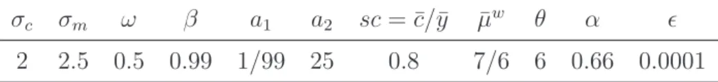
σc σm ω β a1 a2 sc= ¯c/y¯ µ¯w θ α ²
2 2.5 0.5 0.99 1/99 25 0.8 7/6 6 0.66 0.0001 Table 1: Baseline calibration
In our baseline calibration we setθ = 6 andα= 0.66, where the latter can be found for example in Walsh (2005) or Woodford (2003a). The parameter a2 is set such that
agents work 1/3 of their available time in the steady state.
We calibrate the money demand block of our model to be in line with the existing literature and U.S. times series data. In particular, we set the annual interest semi-elasticity of money demand,∂logm/∂R=−[R(R−1)σm]−1 equal to - 4.47 at an annual
interest rate of R = 1.083. This is in line with Lucas (2000) and Woodford (2003a). In calibrating this elasticity we have assumed an average annual inflation rate of 4 per cent 2The first conditions and the constraints of the Ramsey problem in the deterministic steady state
together with a real interest rate of 4.3 per cent such that R = 1.083. It then follows that σm = 2.5. Note that the semi-elasticity and the elasticity of money demand,
ηR(R) ≡ [(R−1)σm]−1 > 0, increases (in absolute terms) as interest rates decrease.3
We assume a degree of relative risk aversion σc = 2. This implies an output elasticity
of money demand σc/(scσm) = 1. Furthermore, we set the parameter a1 = 1/99 such
that at a nominal interest rate ofR= 1.083 the annual ratio ofM1 over nominal GDP equals 0.2. This value is consistent with postwar U.S. data and similar to the one used by Schmitt-Groh´e and Uribe (2004, 2005).
Then the following numerical result for the ²steady state holds:
Result 1 (Optimal Steady State) If a1 ≥ 1/3513 and the other parameters are
given by the baseline calibration, optimal inflation in the deterministic steady state
π is β +² = 0.9901. The associated optimal price dispersion ∆¯ is 1.0014, while the optimal nominal interest rate R¯ is 1.0001>1.
Details of the computation can be found in appendix 6.2.4 Under the baseline
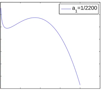
calibra-tion, we find that the optimal steady value for inflation is the lower bound, π=β+², i.e. it involves deflation. Correspondingly, the nominal interest rate is almost zero. We obtain this result even if when assuming a low weight for the utility of real money balances. Basically, Schmitt-Groh´e and Uribe (2004, 2005) and Khan et al. (2003) find that the optimal inflation rate is close but not identical to unity, where the welfare function has slope zero, the interior solution (see Figure 1). In this steady state, the predominant aim of policy is to minimize price dispersion. However, if the weight as-signed to the utility of real money balances is large enough – larger than 1/3513 – this 3Note that this is not due to the fact that we use a separable MIU formulation. In case of a
non-separable MIU specification, u(c, m); ucm > 0, which is equivalent to a shopping-time or real
resource costs of transactions model (Feenstra, 1986), the corresponding elasticity becomesηR(R) =
[(R−1)(σm+²cm)]−1,²cm=ucmm/uc.
0.99 0.995 1 1.005 1.01 1.015 −0.912 −0.9115 −0.911 −0.9105 −0.91 −0.9095 −0.909 −0.9085 Inflation u( π ) a 1=1/2200
Figure 1: Welfare and Inflation in the steady state
optimum becomes a local maximum only, while the global optimum is the Friedman Rule.
Since a1 is an unobserved preference parameter, it is difficult to assess whether the
critical valuea1 = 1/3513 implies a large or small role for money in the utility function.
However, the annual steady state ratio ofM1 over nominal GDP implied by this critical value is 0.048. Hence, even if the importance of money in transactions - as measured by this ratio - falls by 76% from its baseline value of 0.2, the Friedman rule would still be optimal. Therefore, the Friedman rule is optimal in our model even when money provides a very small flow of utility.
Why does the Friedman rule turn out to be optimal even when the importance of real money balances in the utility function is very low? Optimal monetary policy seeks to minimize two distortions created by price dispersion and the transaction friction, since the monopolistic distortion is eliminated by an output subsidy.5 Price dispersion
5The output subsidy of τ= 1−(1−αβπθ−1)µwθρ(π)1/(θ−1)[(1−αβπθ)(θ−1)]−1<0 depends on
calls for an inflation rate of zero, while the monetary friction requires deflation. Corre-spondingly, we expect our optimal gross inflation rate to be found betweenβ and unity. First, while studies such as Kiley (2002) and Ascari (2004) have shown that relatively small amounts of trend inflation are associated with relatively large welfare costs under Calvo pricing, this is not the case for long run deflation. Figure 4 in the appendix shows that the price dispersion arising from long run deflation is relatively small. The second reason for the optimality of Friedman’s rule is an adaption of a general principle of optimal taxation in public finance. Since the interest rate acts like a tax on money holdings, it should be low due to the fact that money demand is elastic with respect to interest under price stability.
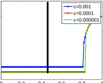
While the choice for²is arbitrary, our results are not very sensitive to the magnitude of ² (see Figure 5 in the appendix). The graph plots optimal annual inflation against the degree of price dispersion α. Remarkably, our threshold levels for the optimality of Friedman’s rule differ substantially from the results obtained by Schmitt-Groh´e and Uribe (2005, Figure 1). While the Friedman rule in our model is optimal until the degree of price dispersion is below 0.81, Schmitt-Groh´e and Uribe find a considerably lower breaking point of approximately 0.46 (see the vertical line in Figure 5), since the welfare costs of positive interest rates are lower in their transaction costs specification. Which parameters influence the lower bound on a1, i.e. the minimum weight for
money in the utility function that renders the Friedman rule optimal? Put differently, which structural features work in favor for the Friedman rule and when does price dis-persion become the main focus of monetary policy? To gain intuition for this question, we compare the outcomes of the Friedman rule and a zero inflation policy and derive an
we were to apply the subsidy under zero-inflation,τ = 1−µwθ/(θ−1), the Friedman Rule would be
optimal for even smaller relative weights of money in the utility function. The reason is as follows. First, note that steady state output is lower when the subsidy does not depend on trend deflation. Note further that the utility loss that households suffer due to a positive steady state price dispersion is weighted with the steady state output.
analytical expression of the threshold for which the former dominates the latter policy.
Proposition 1 (Friedman’s Rule and Zero Inflation) Assume that preferences are
of the separable CRRA type and logarithmic,σm =σc= 1, anda2 = 1. Then the
Fried-man Rule steady state, πF R =β+², yields higher utility than the zero inflation steady
state, πZERO = 1, if and only if
a1 > a1 ≡
∆F R−1
(1+ω)sc +1+ωω ln[∆F R]
ln[RF RηR,F R(RZEROηR,ZERO)−1]−ω/(1 +ω) ln[∆F R]
with∆F Ras the price dispersion associated withπ =β+²andRF RηR,F R(RZEROηR,ZERO)−1 =
(1−β)(1 +β−1²)/β−1².
Proof see appendix 6.4.
RZERO = β−1 and RF R = 1 +β−1² denote the gross nominal interest rate under zero
inflation and Friedman’s rule. Evidently, the Friedman rule performs better than a zero inflation regime, when the degree of price dispersion associated with the Friedman rule, ∆F R is small. But at least equally important is the sensitivity of money demand with
respect to interest rates under Friedman’s rule, ηR,F R, compared to the corresponding
elasticity if zero inflation applies, ηR,ZERO. If these elasticities differ substantially,
the amount and utility of real money balances in both regimes differs too. As will become clear below, this elasticity heavily influences the possible welfare losses due to positive interest rates. Furthermore, a large fraction of private consumption, sc, favors the Friedman rule. The intuition is as follows. Consider a value fora1 such that
the Friedman rule delivers the same steady state welfare as the zero inflation policy. If the fraction of government expenditures decreases, people have to work less since less output has to be produced. Due to price dispersion, people work more under the Friedman Rule, such that their marginal disutility of labor is always higher than under the zero inflation regime. Correspondingly, a one percent decrease in labor in both
regimes leads to relatively larger utility gains in the Friedman Rule regime.
It is important to point out that the Friedman rule is optimal only under com-mitment, but never under discretion. The intuition for this result is that the nominal interest rate as the opportunity cost of money holdings depends on expected inflation. When the central bank acts under discretion, it cannot influence inflation expectations. Hence, the Friedman rule is not optimal under discretion. To see this more formally, consider the optimality condition of the planner’s choice for inflation in the determin-istic steady state under commitment:
λ1K α 1−απ θ−2ρ1−θθ +λ 2αK(θ−1)πθ−2+λ3αF θπθ−1 +λ4[θαπθ−2ρ 1 θ−1 −αθπθ−1∆]−λ5Ruc π2 . = 0. (15)
Here, the multipliersλ4 >0 andλ5 >0 measure the severeness of price dispersion and
the transaction friction in terms of utility. A necessary requirement for the Friedman rule to qualify as an optimum is that (15) is non-positive for π → β. Otherwise, it is always possible to increase welfare by increasing inflation. Therefore, a high value of λ5 relative to λ4 for all inflation rates between β and 1 favors the lower bound as the
optimum. While λ4 is mainly driven by the degree of price stickyness α, λ5 crucially
depends on the elasticity of money demand with respect to the nominal interest rate, λ5 = mzmηR. In order not to distort behavior money holdings should not be taxed
with positive interest rates if they are demanded elastically. Note that this reasoning is based on an expectation argument, which does not arise if the central bank acts under discretion. In that case, the central bank does not consider the impact of its actions on expected inflation. Hence, the first order condition for inflation
λ1K α 1−απ θ−2ρ1−θθ +λ 4[θαπθ−2ρ 1 θ−1 −αθπθ−1∆], (16)
is not affected by the multiplier λ5, i.e. by considerations that seek to eliminate the
monetary distortion. Under discretion, the multiplier λ5 does not appear since it is
associated with future inflation. Correspondingly, the following proposition states that under discretion the Friedman rule is not optimal in our economy – independent of the size of the relative weight for the utility of real money balances.
Proposition 2 (Optimal Steady State under Discretion) Consider the
optimiza-tion under discreoptimiza-tion and suppose that a1 and sc are finite. If the preferences are of
the separable CRRA type andσcsc−1 ≥1, then the Friedman Rule is not optimal in the
deterministic steady state.
Proof see appendix 6.5.
In the following subsection we consider optimal monetary policy in the short run, as-suming the baseline calibration, such that β+² is the optimal inflation rate from a timeless perspective.
3.2
Approximating the model around the optimal steady state
The model is log-linearized around the optimal deterministic steady stateπ =β+² <1, i.e. under trend deflation and closely follows the approximation around trend inflation (Ascari, 2004). The rational expectations equilibrium for the log-linear-approximate model is then a set of sequences{ybt,πbt,mbt,Rbt,Fbt}∞t=t0 consistent with the following set of equilibrium conditions6 σ(Etbyt+1−byt+gt−gt+1) =Rbt−bπt+1, (17) b mt= σ σm (ybt−gt)−ηR,F RRbt, (18)b πt=βEtbπt+1+κ∗(ω+σ)(byt−bytz) + κ∗(¯π−1) 1−αβπθ[(σ−1)ybt+Fbt] (19) b Ft= (1−αβπθ)[(1 +ω)ybt+µbwt −(1 +ω)bat)] +αβπθEt(θπbt+1+Fbt+1), (20)
where ηR,F R = [σm(RF R −1)]−1, sc = c/y, σc = −uccc/ucc > 0, σ = σcsc−1, ω =
vlll/vl >0, gt = (Gt−G)/y+σ−1ζbt, κ∗ = (1−απθ−1)(1−βαπθ)/(απθ), disturbances
are collected in ybz
t = ((1 +ω)bat +σgt −µbwt)/(ω + σ), σm = −zmm( ¯m) ¯m/zm( ¯m) >
0, the transversality condition, for a monetary policy, a sequence {ξbt}∞t=t0, and given initial values Mt0−1 and Pt0−1. Further zbt denotes the percent deviation of a generic variablezt from its steady state valuez. In addition we assume that the bounds on the
fluctuations of the shock vector klogξtk are sufficiently tight, such that ξt remains in
the neighborhood of its steady state value.
3.3
The Quadratic Policy Objective
In this section we derive a purely quadratic welfare measure for the utility of the average household as the relevant objective for optimal monetary policy in the short run.
We assume that the welfare-relevant objective is the expected and discounted aver-age utility level of all households, which is given by
Uto ≡Et0 ∞ X t=t0 βt−t0{u(c t, ζt)− Z 1 0 v(ljt)dj +z(Mt/Pt)}. (21)
Our aim is to derive a quadratic loss function that yields an accurate second order approximation of the average utility of all households. We seek to evaluate the ap-proximated level of utility by using the log-linearized conditions (17)-(20) describing the competitive equilibrium – that is, we set up the familiar linear-quadratic optimal policy problem. A correct welfare ranking of alternative policies requires a second-order approximation of utility that involves no linear terms – at least in expectations (see
Woodford, 2003a, ch.6).
The existence of a non-zero linear term in the utility approximation crucially relies on the distortions of the steady state output relative to the efficient output level as con-sequences of price and wage-setting power, distortionary taxation and trend deflation that are represented in φ:
1−φ=ρ(π)1−1θ(1−τ)θ−1 µwθ 1−αβπθ 1−αβπθ−1 = vl uc . (22)
If this inefficiency gap is zero or only of first order inφ, the linear term in the second order approximation vanishes. Following Rotemberg and Woodford (1997) we assume that the sales tax plays a role of an output subsidy that offsets exactly the steady state output distortion. Since we assume separability between consumption and real money balances, this implies that real balance effects do not contribute to this inefficiency measure.
As Carlstrom and Fuerst (2004) point out, the inclusion of money demand funda-mentally changes optimal monetary policy responses even in case if one assumes – as we do – real balances do not effect the dynamic evolution of inflation and output in the competitive equilibrium. The reason is that variations in the nominal interest rate contribute to the relevant distortions the policy maker seeks to stabilize. As we will show below, the relative weight of variations in the interest rate that enters the welfare measure is substantially increased if we approximate around the optimal steady state. In the following proposition we derive a quadratic Taylor-series approximation to (21).
Proposition 3 (Quadratic Approximation to Utility) If the fluctuations inytaround
y, Rt around R, ξt around ξ, πt around π are small enough, π and ∆ are close enough
subsidy τ, the utility of the average household can be approximated by: Ut0 =−ΩEt0 ∞ X t=t0 βt−t0[λ x(byt−byt∗)2+πbt2+λRRb2t] +t.i.s.p.+O(kξbt, ςk3), (23)
wheret.i.s.p.indicate terms independent of stabilization policy, κ= (1−α)(1−αβ)(ω+ σ)/α, Ω = ucyθ(ω+σ) 2κ , λx = κ θ, (24) λR= ηR,F Rλx v(ω+σ), (25) and b yt∗ = σgt+ (1 +ω)bat ω+σ , (26) where v =y/m >0.
Proof see appendix 6.7.
Under the conditions given in proposition 3, the relative weights of inflation, output gap and the nominal interest rates correspond to the results in Woodford (2003a). Our analysis differs from Woodford (2003a), because the steady state values relate to the lower bound and no longer to price stability as in his analysis. A crucial feature for the validity of the quadratic approximation above is that price dispersion in the optimal deterministic steady state (involving deflation) is not too large. Since the dispersion measure is lower for deflation than for inflation (see Figure 4 in the appendix) this is more likely to be fulfilled when the model is approximated around a deflationary steady state.7
Remarkably, only the weight to stabilize fluctuations in the nominal interest rate 7In addition, we checked the accuracy of the results by comparing them to the optimal solution
implied by the procedure proposed by Khan et al. 2003. We thank Andrew Levin for providing us with the MATLAB codes that solve the Ramsey problem in Levin et. al. (2005)
depends on steady state values, v and ηR,F R. Since we approximate our model around
the deterministic steady state consistent with the Friedman Rule, the value for the former is small and even more importantly the value for the latter is large, implying a high preference to stabilize variations in the opportunity costs to hold money: For π → β, this preference becomes even infinitely large. Notably, the dependence of the stabilization weights on the approximation point is absent in cashless economies: The weights for inflation (1) and output gap stabilization (κ/θ) do not hinge on steady state values. To set up the optimal policy problem, we need to rewrite the relevant constraints, i.e. the Euler-equation, the law of motion forFbt and the aggregate supply
curve in terms of the welfare-relevant output gap,xt =ybt−yb∗t:
b Rt=bπt+1+σ(Etxt+1−xt) +nt, (27) b Ft= (1−αβπ¯θ)(1 +ω)xt+ut+αβπ¯θEt(θπbt+1+Fbt+1) (28) and b πt=βEtbπt+1+η4xt+ κ∗(¯π−1) 1−αβπ¯θFbt+st. (29)
Here, nt, ut, st denote linear combinations of the elements of ξbt and η4 is a constant,
which are defined in appendix 6.8. Note, that the money demand condition does not enter the set of relevant constraints of the policy problem. Nevertheless it influences the optimal decision via the quadratic loss function, in which it plays an important role in determining the relative weight of interest rate variations.
4
Optimal short-run policy from a timeless
perspec-tive
We are interested in the optimal policy from a timeless perspective (Woodford, 2003a) in a linear quadratic framework. We showed that the optimal policy in the long run is to follow the Friedman rule. In this section we consider the implications for optimal policy in the short run, if deflation – instead of zero inflation – is chosen as the optimal long target. In particular, we consider the optimal reaction to various kinds of disturbances and evaluate the resulting stabilization loss of both regimes.
4.1
Optimal response to shocks
This subsection discusses the optimal response to shocks in the economy. We present the impulse responses under optimal policy under commitment and distinguish two cases. In the first case, our set of equilibrium conditions is log-linearized around the optimal steady state in which the inflation rate is equal toβ+². In the second case, we follow the conventional procedure and approximate around a steady state of zero inflation. The choice of a point of expansion for the log-linearization affects both the loss function and equilibrium conditions. Log-linearizing round the Friedman rule increases the relative weight on the stabilization of the nominal interest rate and affects the coefficients in the Phillips curve.
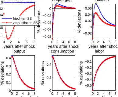
When we log-linearize around the optimal steady state corresponding to the Fried-man rule, we find that the central bank essentially keeps the nominal interest rate fixed in response to any of the shocks present in our model. Consider first the optimal response to a technology shock displayed in Figure 2.
A Taylor expansion around zero inflation suggests that central bank should lower the annualized nominal rate by roughly 12 basis points and then gradually return to
0 2 4 6 8 −0.1 −0.08 −0.06 −0.04 −0.02 0 interest rate
years after shock
% deviations friedman SS zero inflation SS 0 2 4 6 8 −0.08 −0.06 −0.04 −0.02 0 output gap
years after shock
% deviations 0 2 4 6 8 −0.02 0 0.02 0.04 0.06 inflation
years after shock
% deviations 0 2 4 6 8 0 0.1 0.2 0.3 0.4 output
years after shock
% deviations 0 2 4 6 8 0 0.2 0.4 consumption
years after shock
% deviations 0 2 4 6 8 −0.5 −0.4 −0.3 −0.2 −0.1 labor
years after shock
% deviations
Figure 2: Responses to technology shock
the steady state. However, linearization around the Friedman rule implies that the nominal rate is literally fixed. In line with this finding, the approximation around the Friedman rule implies more volatile response of inflation and the output gap than what is suggested by linearization around the zero inflation steady state. A stronger stabilization of the nominal interest rate necessarily implies that the other arguments in the loss function can only be stabilized less.
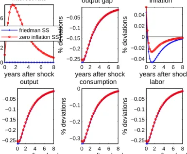
Impulse responses to the other shocks deliver a similar message: Linearization around the Friedman steady state implies that the nominal interest rate is literally fixed. Inflation and output gap fluctuate by more than when the linearization is performed around the zero inflation steady state. The reason for why the interest rate does not respond under optimal policy is that stabilization of the interest rate is the main prin-ciple (see Table 2). Intuitively, the interest elasticity of money demand, [σm(R−1)]−1
becomes very large asR approaches its lower bound. For our baseline calibration this elasticity is roughly -4000 at R = 1 +². Despite the fact that the marginal utility of
0 2 4 6 8 0 0.02 0.04 0.06 interest rate
years after shock
% deviations friedman SS zero inflation SS 0 2 4 6 8 −0.25 −0.2 −0.15 −0.1 −0.05 output gap
years after shock
% deviations 0 2 4 6 8 −0.04 −0.02 0 0.02 0.04 inflation
years after shock
% deviations 0 2 4 6 8 −0.25 −0.2 −0.15 −0.1 −0.05 output
years after shock
% deviations 0 2 4 6 8 −0.3 −0.2 −0.1 0 consumption
years after shock
% deviations 0 2 4 6 8 −0.25 −0.2 −0.15 −0.1 −0.05 labor
years after shock
% deviations
Figure 3: Responses to wage markup shock
real balances is close to zero (such that v is small), this large elasticity explains why the central bank wishes to hold the nominal rate constant under the Friedman rule.
4.2
Welfare Analysis
In this subsection we compare the welfare implications of the two policy regimes – the long run deflation target according to the Friedman rule vs. zero inflation as the long run target. Using (23) a second-order accurate approximation to the utility of the average household is given by:
Ut0 =Et0 ∞ X t=t0 βt−t0U t ≈ 1 1−βU¯ −ΩEt0 ∞ X t=t0 βt−t0λ x(byt−ybt∗)2+πbt2+λRRb2t. (30)
The first part, the discounted steady state utility, is shown to be higher if the Friedman rule is optimal. The second part, the stabilization loss, that relates to the optimal policy reaction in the short run, is not necessarily lower under the Friedman rule regime than
under zero inflation. Which of those two parts dominates depends on the calibration of the model, e.g. increasing the variances of the innovations amplifies the welfare loss due to short run fluctuations. In line with the spirit of the timeless perspective, we do not compute welfare conditional on a particular initial state vector at time t0. Our short
run stabilization loss is given by the discounted and weighted sum of unconditional variances:
SL=− 1
1−βΩ{var(πb) +λxvar(x) +λRvar(Rb)}=− 1
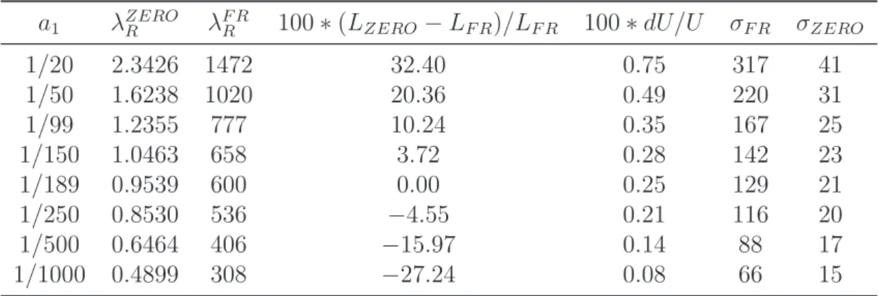
1−βΩL, (31) Here L is proportional to the unconditional expectation of period utility. In table 2 below we list the relative loss differences under the two policy regimes for a range of relative weights for the utility of real money balances given our baseline calibration for other parameters. For this purpose we calibrate the stochastic shock processes to match the standard deviations of real private consumption and government spending of U.S. data during the post-Volcker period.8 All exogenous processes are assumed
to be autocorrelated with coefficient 0.9. We have chosen a standard deviation of the innovations to the taste shock of 0.0001, for the markup shock 0.00015, for the government spending shock 0.0075 and for the technology shock 0.0096.
8The quarterly data is logged and detrended via the Hodrick-Prescott filter with a smoothing
parameter of 10,000. The obtained standard deviation of private consumption is 0.0123, for government expenditures we obtain 0.0172.
a1 λZEROR λF RR 100∗(LZERO−LF R)/LF R 100∗dU/U σF R σZERO 1/20 2.3426 1472 32.40 0.75 317 41 1/50 1.6238 1020 20.36 0.49 220 31 1/99 1.2355 777 10.24 0.35 167 25 1/150 1.0463 658 3.72 0.28 142 23 1/189 0.9539 600 0.00 0.25 129 21 1/250 0.8530 536 −4.55 0.21 116 20 1/500 0.6464 406 −15.97 0.14 88 17 1/1000 0.4899 308 −27.24 0.08 66 15
Table 2: Welfare Analysis: ²= 0.0001
The results in Table 2 reveal that the larger the preference parameter of the house-holds’ for the Friedman rule steady statea1 the larger is the willingness of the central
bank to stabilize the nominal interest rateλF R
R . This implies that optimal long run and
short run monetary policy are closely interrelated in case of a transaction friction9.
The resulting stabilization loss, when approximating around the Friedman rule steady state LF R is superior to the stabilization loss around zero inflation LZERO if
a1 is large enough. The (technical) intuition for this is a trade off effect between
pre-dictability and possible welfare losses in the neighborhood of the steady state of each regime. If the Friedman rule is the expansion point, then the reduced form involves 4 jump variables,Rbt,xt,bπtandFbt, as well as 3 endogenous state variables, the multipliers
on the relevant constraints, (27)-(29). If zero inflation is chosen as the approximation point, the reduced form does not involve Fbt and exhibits only the two multipliers
as-sociated with the aggregate supply curve and the euler equation as endogenous state variables. On the one hand, the state space is increased in the Friedman regime, im-plying higher prediction power by reducing the error variances of inflation, output gap and the nominal interest rate.10 On the other hand, however, possible welfare losses
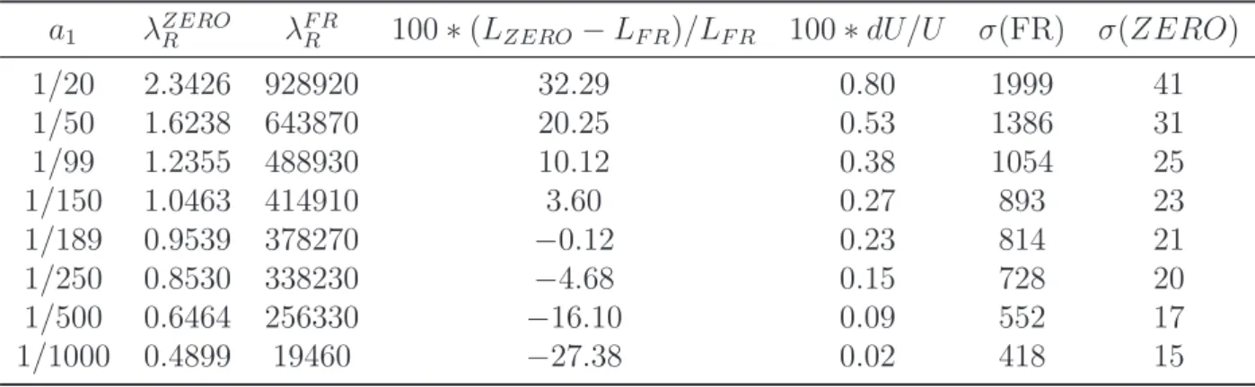
9Table 3 in the appendix gives the corresponding results for ²=.000001, i.e. if the assumed lower
bound is closer to the zero bound.
in the neighborhood of the zero inflation steady state are lower, steady state utility is ”flatter” around π = 1 (see Figure 1). If the relative weight of real money balances decreases, the additional state variable loses prediction power, while possible welfare losses around the zero inflation steady state decrease. Intuitively, the prediction effect is larger, if the endogenous state variables carry the main relevant information from previous periods, i.e. if the disturbances are only weakly autocorrelated. While there is a cut-off value in terms of stabilization loss, overall utility composed of steady state utility minus stabilization loss, is higher under the Friedman rule than under zero in-flation though the relative differences are small. The second but last column of Table 2 depicts this overall difference in utility under the Friedman regime minus the zero inflation regime expressed as percentages.
The entries σF R and σZERO shed light on how likely it is that the lower bound on
the nominal interest rate binds if the economy fluctuates around the Friedman rule ² steady state or around price stability. We calculate the standard deviation of the nominal interest rate under the optimal policy implied by both policy regimes. The term σF R then expresses the size of the interval from R = 1.0001 to the lower bound
R= 1 in terms of this standard deviation. The entryσZERO also expresses this interval
in terms of standard deviations of the nominal rate, but now the approximation is computed around a zero inflation steady state. Hence, larger values for σF R or for
σZERO imply that the lower bound is less likely to be binding. Note that our results
imply a low probability that the nominal interest rate hits the lower bound, i.e. Rt= 1.
Even for a small relative weight of real money balances, a1 = 1/1000, the resulting
standard deviation for the nominal interest rate is small relative to ², such that a symmetric confidence interval aroundR = 1.0001 of up to 66 standard deviations could be constructed until the lower bound is included. If we decrease², i.e. if the assumed
lower bound moves closer to zero, the corresponding number of standard deviations increases to 418 (see table 3 in the appendix). This implies that the effect to stabilize the nominal interest even more (higher relative weight λF R
R ) dominates the effect of
the smaller distance to the zero bound. Correspondingly, if zero inflation is chosen as the expansion point, the probability to hit the lower bound is even higher (see the last column).
5
Conclusion
We study optimal monetary policy in an economy without capital, where firms set prices in a staggered way without indexation and real money balances are assumed to provide utility. Accounting for a sizeable degree of nominal rigidity, the optimal deterministic steady state from a timeless perspective is to follow the Friedman rule, even if the importance assigned to the utility of money is small relative to consumption and leisure.
We approximate the model around the optimal steady state under commitment as the long-run policy target and derive a second order approximation to households’ utility. Optimal interest rate policy is shown to abstain from reacting sharply to changes in the state of the economy. Instead of stabilizing inflation, the primary goal of the central bank is to stabilize fluctuations in the nominal interest rate. In that light, the well observed tendency of central banks to keep the main refinancing instrument literally fixed over a long time can be interpreted as optimal behavior according to Friedman’s rule, even if the state of the economy has changed. Since optimal policy stabilizes fluctuations in interest to a large amount, the lower bound on the nominal interest rate is unlikely to be binding.
monetary policy. It is too stylized for this purpose. The foremost contribution of this paper is to challenge the conventional view that the Friedman rule loses out to the goal of price stability once price stickiness is introduced. We show that the widely used money-in-the utility function model implies that the Friedman rule is optimal even when large amounts of price stickiness are present. When the economy fluctuates around the Friedman rule steady state, central bankers should keep the nominal interest stable over the business cycle. This result is explained by the large interest elasticity of money demand that obtains in the MIU model when the nominal rate is close to zero. There is little empirical evidence on the behavior of money demand in the major industrialized countries for very low interest rates. This is unfortunate as the interest elasticity at low interest rates is a key difference between our MIU framework and the transactions technology employed in other papers that come to different policy prescriptions. Hence, future research on optimal policy in sticky price models benefits from a better understanding of money demand in such low interest rate environments.
6
Appendix
6.1
The optimal deterministic state from a timeless
perspec-tive
The standard commitment approach would be to choose state contingent path for ∆t, Rt, πt and yt for each t ≥ t0, to maximize (8) for a given degree of initial price
dispersion an initial nominal interest rate. Without any precommitment, this approach would suffer of time inconsistency. Woodford (2003) proposes a certain degree of initial commitment, to bring about the optimal equilibrium. In our case, we need to assume,
thatFt0 =F,Kt0 =K andyt0 =y,i.e. the initial values for these variables are identical their optimal steady state values. The optimal deterministic steady state is a solution to the problem defined in the text, that involves constant values for all variables and each of the disturbances identical to their means. Basically we are looking for an initial degree of price dispersion ∆t0−1 and an initial interest rate Rt0−1, and precommitment
Ft0 =F, Kt0 =K and yt0 =y, such that Rt=R, πt=π, Ft=F,Kt =K, yt =y, for each period, and ∆, R are equal to the initial price dispersion an the initial nominal interest rate. Using the time-invariant form for the Lagrangian, the first order necessary conditions with respect toyt, ∆t,Kt,Ft, Rt and πt for all t≥t0 are given by:
uc(t)−∆tvl(t) +zm(t)mc(t) +λ2t(1−τ)[ucc(t)yt+uc(t)] +λ3tµwt[vll(t)∆tyt+vl(t)]−λ5tucc(t) +λ5t−1 ucc(t)Rt−1 πt . = 0 (32) −ytvl(t) +λ3tvll(t)yt2µwt +λ4t−λ4t+1βαπtθ+1 = 0. (33) λ1tρ(t) 1 1−θ −[λ 2t−απθt−1λ2t−1]= 0. (34) − θ θ−1λ1t−[λ3t−απ θ tλ3t−1]= 0. (35) zm(t)mR(t) +λ5tβuc(t+ 1) πt+1 . = 0 (36) and λ1tKt α 1−απ θ−2 t ρ(t) θ 1−θ +λ2t−1αKt(θ−1)πθ−2 t +λ3t−1αFtθπθt−1 +λ4t[θαπθt−2ρ(t) 1 θ−1 −αθπθ−1 t ∆t−1]−λ5t−1Rt−1 uc(t) π2 t . = 0. (37)
Note thatλ2t0−1, λ3t0 and λ5t0−1 are the multipliers associated with the initial commit-ment.
6.2
Description of the numerical procedure to calculate the
optimal steady state
We solved for the optimal deterministic steady state numerically. Thereby we used the specific CRRA utility function given in the text.
The procedure works in the following way: We solve for y,R, F, K and ∆ each as a function of steady state inflation exclusively – using the constraints (9)-(13). That is, for a given inflation rate, the values for the other variables are given by these functions. To check for the robustness of out results, we use two different procedures: The first one involves the exploitation of the first order conditions, the second one the direct evaluation of utility in the steady state.11
The first procedure is applied in the programstcommit.m. We use the values given by the constraints and solve for the lagrangian multipliersλ1-λ5 uniquely by exploiting
the 5 first order conditions for output, interest, dispersion,F andK. Then we use these values and substitute them in the first order condition for inflation,f c(π), to check for optimality of the given inflation rate. Thereby several cases are possible. For example, if this condition is globally negative (positive) over the grid of steady state inflation rates, then the optimal inflation is the lower (upper) bound. If however, the first order condition crosses the zero line, the optimum can be an interior solution. Suppose that f c(π) is positive at the lower bound, monotonically decreasing and crosses the inflation axis at some inflation rate,π1 ∈(β+²,upper bound). Thenπ1 is the optimal inflation.
If instead, f c is negative at the lower bound, monotonically increasing and crosses the zero value for π2, thenπ2 can’t be the optimum – either the lower bound or the upper
bound is the optimum. Obviously – in principle – several cases are possible and even multiple solutions can arise. Once, the optimal inflation rate is found, the values for 11The MATLAB programs to compute the optimal steady state, and the Toolkit code to calculate
the variables and the lagrangian multipliers are implied by the constraints or the first order conditions.
The program ssrand31.m uses a direct evaluation of steady state utility by substi-tuting for each given inflation rate, the values of output, interest,F, K and dispersion into the utility function. Afterwards one maximizes over the resulting utility function and picks the optimal inflation rate and the optimal values for the variables are implied b