ISSN 1745-8587
Birkbeck Workin
g
Pa
p
ers in Economics & Finance
Department of Economics, Mathematics and Statistics
BWPEF 1401
Balanced budget stimulus with
tax cuts in a liquidity-constrained
economy
Vivek Prasad
Birkbeck, University of London
Balanced budget stimulus with tax cuts in a liquidity
constrained economy
∗Vivek Prasad†
(Preliminary draft, for discussion, not for quotation)
January 31, 2014
Abstract: This paper examines the macroeconomic effects of unexpected, exogenous, simul-taneous, temporary cuts to income tax rates in an economy when the government follows a balanced budget fiscal rule and keeps money supply constant, and private agents face con-straints on the ability to finance investments. The main results are that the tax cuts increase output, private consumption, and investment; the increases in output and consumption are sig-nificant and long-lasting; and the liquidity constraints play a major role in the shock’s long-term persistence. Results are obtained from calibrating a modified version of the DSGE model of liquidity and business cycles byKiyotaki and Moore(2012). The modifications are twofold: (i) distortionary taxes to labour and dividend incomes are added, and (ii) the government follows a balanced budget fiscal rule and keeps money supply constant. Results are qualitatively robust, but quantitatively sensitive, to assumptions regarding structural parameter values, and quali-tatively and quantiquali-tatively sensitive to significant variations in the persistence of tax shocks.
JEL Classification: E10, E20, E30, E44, E50, E62, H30
Keywords: Fiscal policy, taxation, balanced budget, liquidity constraints
∗
I am grateful to John Driffill and Ron Smith for their guidance throughout this paper, and to Ivan Petrella, Stephen Wright, and seminar participants at Birkbeck for useful comments. All errors and omissions are my own.
†
Department of Economics, Mathematics and Statistics, Birkbeck College, University of London, Malet Street, London WC1E 7HX. E-mail: v.prasad@mail.bbk.ac.uk.
1
Introduction
This paper examines the macroeconomic effects of cuts to income tax rates in an economy when the government follows a balanced budget fiscal rule and keeps money supply constant, and private agents face constraints on the ability to finance investments. The tax rate cuts are unexpected, exogenous, simultaneous, and temporary. The main results are that the tax cuts increase output, private consumption, and investment; the increases in output and consumption are significant and long-lasting; and the liquidity constraints play a major role in the shock’s long-term persistence. Liquidity constraints create demands for two assets of varying liquidity; tax cuts increase the demand for both assets; and while the tax cuts also lead to an increase in supply of the less liquid asset, the liquidity constraints restrict this increase to be small; ac-cordingly, both asset prices increase, and amplify the internal propagation of the shock. Results are obtained from calibrating a modified version of the DSGE model of liquidity and business cycles by Kiyotaki and Moore (2012) (henceforth KM). The modifications are twofold: (i) dis-tortionary taxes to labour and dividend incomes are added, and (ii) the government follows a balanced budget fiscal rule and keeps money supply constant. Results are qualitatively robust, but quantitatively sensitive, to assumptions regarding structural parameter values, and qualita-tively and quantitaqualita-tively sensitive to significant variations in the persistence of tax shocks. The paper contributes to an extensive literature on the effectiveness of fiscal policy for economic stimulation. It belongs to a narrow strand of this literature which explores balanced budget ex-pansion. Results are consistent with those achieved byMountford and Uhlig(2009) (henceforth MU) , a member of this balanced budget research.
Tax cuts are shown to be expansionary in early works by Andersen and Jordan (1968),
Giavazzi and Pagano(1990),Baxter and King(1993),Braun(1994),McGrattan(1994),Alesina and Perotti(1997), andPerotti(1999), and more recently byRomer and Romer(2010),Mertens and Ravn (2011a,b,2012), and Monacelli et al. (2012). Support for tax cuts is also expressed in blogs by Hall and Woodford (2008), Bils and Klenow (2008), Mankiw (2008), and Barro
(2009). And counterfactual experiments by Blanchard and Perotti (2002), Romer and Romer
(2010), MU, andAlesina and Ardagna(2010) show that tax cuts produce larger responses than increases in government spending.
Tax cuts with a balanced budget are shown to be expansionary in Eggertsson (2010) and MU. Eggertsson (2010) obtains his results by cutting consumption taxes and simultaneously raising income and wealth taxes to perfectly compensate. MU show that completely financing an unexpected, exogenous increase in government spending with an increase in taxation causes reductions in private consumption and investment on impact, as well as in output from the second period.1 The converse of this result suggests a recipe for debt-free economic expansion. This paper complements MU by showing that the converse of their result is also true. The novelty of this paper is that while MU obtain their results from an empirical study with vector autoregressions, this paper is a theoretical investigation using a mostly neoclassical DSGE model.
The KM model is chosen for its pair of financial frictions, which resemble an essential 1
feature of the 2007/8 financial crisis. This makes the paper relevant for policy discussions on the crisis. KM is an otherwise neoclassical model, but with constraints on firms’ ability to internally and externally finance investments. Commentators argue that the cause of the crisis was the sudden and unexpected deterioration in the value of partially liquid private financial assets, which thus ruined their resaleability and suitability for use as collateral (Brunnermeier
(2009), Del Negro et al. (2011), Bigio (2012) and Jermann and Quadrini (2012)). Assets’ resaleability and suitability for collateral were thus adversely affected. This event bears a striking resemblance to KM’s own negative liquidity shock.
The KM model is theoretically adjusted and/or extended in a series of recent papers. These papers can be classified into two groups. The first group uses the KM model to evaluate the unconventional policies seen in the crisis; Del Negro et al.(2011) andDriffill and Miller(2013) are members of this research, and both show that recessions would have been exacerbated had it not been for government interventions. The second KM-related group returns to the original questions posed by KM on the importance of (i) liquidity shocks for explaining business cycles, and (ii) liquidity constraints for the propagation of productivity shocks. Papers in this group includeSalas-Landeau(2010),Bigio(2010,2012),Ajello(2011),Nezafat and Slav´ık(2012),Shi
(2012), andJermann and Quadrini (2012).
The inclusion of distortionary taxes and a balanced budget rule is not unique in KM-related literature. Ajello (2011), Shi (2012), and Driffill and Miller (2013) have a balanced budget rule for government. Ajello (2011) also includes distortionary taxes, but he modifies the KM model more extensively than in this paper. The uniqueness of this contribution is that it is the first to examine fiscal shocks in the KM model. What is shares with these papers, the second KM-related group in particular, is showing the macroeconomic significance of KM’s liquidity constraints in propagating exogenous shocks. In this case, however, the shocks are to tax rates. In a wider literature, the significance of this paper is that it shows how a neoclassical model can be modified to produce large responses to fiscal shocks. The New Keynesian model is the workhorse for fiscal policy research. This perhaps follows from papers likeBurnside et al.(2004), which shows that the magnitude of observed responses to fiscal shocks are not matched by a standard neoclassical models, but they are matched by models that include habit formation and adjustment costs. Beyond the liquidity constraints, this model is otherwise neoclassical. This paper therefore shows that a host of New Keynesian frictions are not always needed to study fiscal policy. The KM model can be a workhorse for that purpose.
The rest of the paper is organized as follows: Section 2 describes the model in full, and derives conditions which characterize the dynamic equilibrium; Section 3 presents the main results of the tax shock; Section4quantifies and comments on the magnitude of shock responses using tax multipliers; Section5briefly gives the conclusions of sensitivity analysis on structural parameters and the persistence of tax shocks; Section6 examines the significance of the results by relating them to similar work in the literature; and Section7concludes the paper and outlines avenues for future research. The technical appendix contains the model’s calibration, sensitivity analysis of the shock, algebra of proofs and derivations, an algebraic solution for steady state, and the data used in the paper.
2
The model
This section defines agents’ behaviour and derives conditions that characterize the dynamic equilibrium. The model is an adaption of the Kiyotaki and Moore (2012) framework with government and without storage. Modifications are twofold: (i) distortionary taxes on wage and dividend income are added, and (ii) different policy rules to the ones in KM are assumed.2 In particular, the government holds no equity, keeps money supply constant, and adheres to a balanced fiscal budget rule. To make the paper self-contained, a full description of the model is given. AppendixCcontains detailed algebra associated with derivations, simplifications, and proofs.
2.1 The environment
The economy exists over an infinite horizon of discrete time periods. It is populated by three groups of infinitely-lived agents: entrepreneurs, workers, and a government. There is no popu-lation growth or decline, and the economy is closed to the rest of the world. Agents produce and consume a perishable general output, which also serves as the numeraire. They also ex-change labour and two assets, equity and money. All markets are competitive and prices are perfectly flexible. There are no financial intermediaries; instead, agents borrow directly from other agents. The economy is also subject to random, stochastic shocks.
2.1.1 Entrepreneurs
There is a unit-mass continuum of entrepreneurs. At the start of each period all entrepreneurs are identical. They are the exclusive owners of capital and a homogeneous technology that produces the general output good with guaranteed success. At the beginning of period t the representative entrepreneur ownsktunits of capital and employslthours of labour, and produces
yt units of general output at the end of the period according to
yt=Atktγl
1−γ
t (2.1)
where At is a common level of total factor productivity and γ ∈ (0,1) is the capital elasticity
of output, which, given that the output market is perfectly competitive and the production function exhibits constant returns to scale, is also the share of output accruing to capital. The entrepreneur pays workers wt units of general output for each labour-hour employed. The
quantity of general output left over is the return on the capital used in production; in other words, each unit of capital used in production receivesrtunits of general output as gross profit,
where
rtkt=yt−wtlt (2.2)
Capital depreciates during the production process, and a fraction,δ, of its stock survives to the end of the period when production is complete.
2
KM have two policy rules. One prevents government’s expenditure from exploding, by limiting it to the deviation of their asset holdings from steady state. The other, for open market operations, limits the ratio of current to steady state government equity holdings to a weighted sum of productivity and liquidity impulse responses.
Some time soon after the start of the period, a fraction,π, of entrepreneurs gain access to a homogenous investment technology that converts a unit of general output into a unit of capital with guaranteed success. Entrepreneurs are therefore identical ex ante to when investment opportunities are revealed. π is independently and identically distributed across time and entrepreneurs. Who gets an opportunity to invest is exogenously determined. Those without investment opportunities carry on with what they have been doing since the start of the period, i.e. producing, consuming, and saving (by purchasing assets); they are the period’s “savers”. Those with investment opportunities are the period’s “investors”, and once their behaviour changes to pursue such opportunities. The investment technology is unrestricted in capacity, but its access expires at the end of the period. Afterwards, investors and savers revert to being ex ante identical from the start of the next period.
The production and installation of new capital takes an entire period, so a typical investor who invests itunits of general output has an end-of-period capital stock
kt+1 =δkt+it
To acquire general output for investment, an investor issues new units of equity at the market price. Each of these units has a claim on the future gross profits that it contributed towards creating, i.e. each unit of equity earns rt in dividends after period t’s production is complete.
But equity depreciates in tandem with its underlying capital. Any agent is free to buy equity. An entrepreneur’s holdings of equity issued by other entrepreneurs is called his “outside” equity. The entrepreneur possesses special skills which are costly to replicate and replace. Once an investment project is underway, his human resource is needed for the entire duration to ensure the full amount of new capital is produced. The entrepreneur, however, cannot pre-commit to being involved with the project to its end. Instead, he can guarantee that he will remain with the project for no more than an exogenously determined fraction, θ, of its duration. This implies that he can guarantee a maximum ofθof an investment’s new capital will be produced, which further implies that he can guarantee a maximum ofθ of new output in the next period when the new capital is put to work. Consequently, the investing entrepreneur can credibly raise no more than θ of his investment cost from equity funding. This limitation is called the “borrowing” constraint, and has its origins inHart and Moore(1994) andKiyotaki and Moore
(1997).3
The entrepreneur can internally finance his investment by selling his stock of outside equity. However, the entrepreneur cannot sell all of his outside equity before the window of investment opportunity closes. Instead, he can liquidate up to a fraction,φt, of his holdings. This limitation
is called the “resaleability” constraint, and is an exogenous feature of the model.
Borrowing and resaleability constraints are together called “liquidity” constraints. The fi-3
An alternative interpretation ofθ is constructed by Lorenzoni and Walentin(2007): the entrepreneur can “run away” with a fraction, (1−θ), of the value of his capital at any time, simply because capital is always under his complete control. In models with formal credit markets, unlike this one, θ is featured as a credit market friction: due to a limited ability by lenders to enforce loan contracts, lenders request collateral, and lend at most a fraction,θ, of the value of collateralized assets. The credit market friction is its more common representation, owing to Kiyotaki and Moore (1997) who show its macroeconomic significance, and to Carlstrom and Fuerst
nancing gap they leave is met by the entrepreneur’s stock of a perfectly liquid, government-issued fiat money. While money is intrinsically worthless, its demand is motivated by a precaution against falling short in financing investment opportunities. Moreover, the tighter the liquidity constraints, i.e. the smaller the values of θ and φt, the greater the need to internally finance
investments, and the greater the desire to hold money balances (and conversely). That part of a project that the entrepreneur funds from his own money is called his “inside equity”. It is assumed that inside and outside equity are perfect substitutes, having the same resaleability constraint and providing the same rate of return. Inside and outside equity are therefore col-lectively referred to as “equity”. Equity and money are traded in competitive markets at prices qt and pt, respectively, both expressed in terms of general output.4
For an investment opportunity requiring it units of general output, an entrepreneur will
issue it units of equity. By the borrowing constraint, only a maximum of θit will be sold, and
the investor must therefore retain at least (1−θ)itas new inside equity. The investor will then
liquidate existing equity holdings which have since depreciated. If the entrepreneur holds nt
units of equity at the start of period t then a maximum of φtδnt units can be sold, and the
entrepreneur is left with at least (1−φt)δnt units. The entrepreneur also holds mt units of
money at the start of the period, which cannot be lent or used as collateral. His equity and money holdings at the end of the period are therefore given by
nt+1≥(1−θ)it+ (1−φt)δnt (2.3)
mt+1 ≥0 (2.4)
The gross profit paid to capital at the end of the period represents a dividend payment to the holder of the equity claim on capital. Therefore, an entrepreneur who owns nt units of
equity at the start of the period earnsrtntin gross dividends over the period. He pays a tax on
dividend income to the government at a rate of τtrn. His net dividend income is then allocated to consumption and saving, and to investment if the opportunity exists.
An investor in period t consumes cit units of general output, invests it units, and saves by
acquiring (nit+1−it−δnt) and (mit+1−mt) units of equity and money, respectively, at their
market prices. The investor thus faces a budget constraint for periodt,
cit+it+qt(nit+1−it−δnt) +pt(mit+1−mt) = (1−τtrn)rtnt (2.5)
A saver in periodtconsumescst units of general output, and saves the rest of his net income by purchasing (nst+1−δnt) and (mst+1−mt) units of equity and money, respectively, at their
market prices. The saver’s budget constraint for the period is
cst+qt(nts+1−δnt) +pt(mst+1−mt) = (1−τtrn)rtnt (2.6)
4
In other words,qt andpt units of general output are exchanged for 1 unit of equity and money, respectively.
These are “real” prices. “Nominal” prices are the prices of a unit of general output and equity expressed in terms of money, i.e. 1/ptandpt/qt, respectively. Inflation in the conventional sense is an increase in the nominal price
of general output, or equivalently, a fall in the real price of money (i.e. when a unit of money is exchanged for fewer units of general output).
The representative entrepreneur considers an expected lifetime discounted utility, Et ∞ X j=t βj−tUe(cj) =Ue(ct) +Et[βUe(ct+1) +β2Ue(ct+2) +. . .] (2.7)
whereEt[·] is the expected value conditional on information available in periodt, andβ ∈(0,1)
is the subjective discount factor, or the inverse of the rate of time preference. The investor maximizes Equation (2.7) subject to his budget constraint (2.5) and liquidity constraints (2.3) and (2.4), while the saver maximizes Equation (2.7) subject to his budget constraint (2.6). Each entrepreneur’s current utility is a natural logarithm of current consumption,
Ue(ct)≡lnct
2.1.2 Workers
There is a unit-mass continuum of identical workers. They are the exclusive owners of labour. They do not own capital or have investment opportunities. In period t each worker supplies lwt hours of labour to entrepreneurs in exchange for a gross hourly wage of wt units of general
output. The worker then pays the government a tax on wage income at a rate of τtwl. The worker holds two assets: nwt units of equity and mwt units of money. Each unit of equity earns gross dividends ofrtunits of general output per period, depreciates at a constant rate of (1−δ)
per period, and is subject to the resaleability constraint,φt. Money does not have any of these
features. The worker pays the government a tax on dividend income at a rate of τtrn. The worker’s human resource is non-transferable across time. He therefore cannot borrow or have negative net worth. His equity and money holdings are then always non-negative, i.e. for allt,
nwt ≥0 and mwt ≥0 (2.8)
The worker consumes cwt units of general output. The rest of his net income is saved by purchasing (nwt+1 −δnwt) and (mwt+1 −mwt) units of equity and money, respectively, at their prevailing market prices. His budget constraint is given by
cwt +qt(nwt+1−δnwt) +pt(mwt+1−mwt) = (1−τtwl)wtlwt + (1−τtrn)rtnwt (2.9)
Subject to Equations (2.8) and (2.9), the worker maximises an expected lifetime discounted utility, Et ∞ X j=t βj−tUw(cwj, ljw) =Uw(cwt, lwt ) +Et[βUw(cwt+1, lwt+1) +β2Uw(cwt+2, ltw+2) +. . .] (2.10)
The worker’s utility is additively separable in consumption and leisure,
Uw(cw, lw) =cw−
ω 1 +ν(l
w)1+ν
supply.5
2.1.3 Government
The government is both the monetary and fiscal authority. It costlessly issues fiat money, which it exchanges with the private sector for general output. By issuing (or withdrawing, respectively) money over the period, it earns (or pays, respectively)pt(Mt+1−Mt) units of general output,
where Mt and Mt+1 are the stocks of money in circulation at the start and end of the period,
respectively. Fiat money is the only liability of the government. The only asset it owns is a stock of privately-issued equity. At the start of period tit holdsNtg units of equity, which earn dividends at a rate of rt units of general output over the period, depreciate at a rate of (1−δ)
per period, and are subject to the resaleability constraint,φt. Equity holdings at the end of the
period are therefore lower bounded as
Ntg+1≥(1−φt)δNtg (2.11)
The government holds equity for the conduct of open market operations (OMOs), in which
|Ntg+1−δNtg|units are discretionately exchanged for money.
The government consumes Gt units of general output, and collects Tt in taxes from
en-trepreneurs and workers according to
Tt=τtrnrtNt+τtwlwtLt (2.12)
where Nt is the total private sector’s equity holdings at the beginning of period t, and Lt
is the aggregate number of labour hours used in the period’s production. The government’s spending is assumed to not directly affect the utility of workers and entrepreneurs or create any production externalities.6
The government balances its overall budget in every period. Therefore, its consumption and net OMO purchases is financed from taxes, dividends, and seignorage, according to
Gt+qt(Ntg+1−δN
g
t) =Tt+rtNtg+pt(Mt+1−Mt) (2.13)
2.1.4 Exogenous variables
The economy is subject to exogenous stochastic shocks to {At, φt, Ntg, Mt, τtrn, τtwl}. These
variables evolve according to the same stationary AR(1) process,
At= (1−ρA)A+ρAAt−1+uAt (2.14)
φt= (1−ρφ)φ+ρφφt−1+uφt (2.15)
5
Nezafat and Slav´ık (2012) point out that this utility specification is unusual in the RBC literature, but shows that quantitative results are not sensitive to the choice of functional form. Alternative specifications are the non-separable or log-separable form ofKing et al.(1988) and the form ofGreenwood et al.(1988) whereby disutility from work directly affects utility from consumption.
6
Canova and Pappa (2011) note that if a change in government spending affects private agents’ utility (as inBouakez and Rebei(2007)) and/or creates production externalities (as inBaxter and King (1993)) then the output response is amplified.
Ntg = (1−ρN g)Ng+ρN gNtg−1+u N g t (2.16) Mt= (1−ρM)M+ρMMt−1+uMt (2.17) τtrn= (1−ρτ rn)τrn+ρτ rnτtrn−1+uτ rnt (2.18) τtwl = (1−ρτ wl)τwl+ρτ wlτtwl−1+uτ wlt (2.19)
where, for X ∈ {A, φ, Ng, M, τrn, τwl}, X denotes the steady state value of variable Xt, ρX
parameterizes the degree of persistency of a shock to X, uXt is an exogenously determined, independently, identically, and Normally distributed innovation with zero mean and constant variance σ2uX, and E[uYt uXt ] = 0 for X 6= Y ∈ {A, φ, Ng, M, τrn, τwl}. It is assumed that
|ρX|<1 so that exogenous shocks are temporary.7
2.2 Equilibrium
2.2.1 Entrepreneurs
With the investment technology having unlimited capacity, investors are assumed to liquidate and borrow the maximum amount of equity that the liquidity constraints allow. Then the budget constraint (2.3) becomes binding with equality,
nit+1= (1−θ)it+ (1−φt)δnt (2.20)
which, if re-structured, gives the entrepreneur’s investment for the period,
it= 1 1−θ nit+1− 1−φt 1−θ δnt (2.21)
The investor’s budget constraint (2.5) is simplified by substituting Equation (2.21) to obtain (see Appendix C.1) cit+qtRnit+1= (1−τtrn)rtnt+ φtqt+ (1−φt)qRt δnt+pt(mt−mit+1) (2.22) where qtR≡ 1−θqt 1−θ (2.23)
The RHS of Equation (2.22) is the investor’s net worth: his net dividends from equity holdings, the value of depreciated equity (where a resaleable fraction, φt, is valued at the market price
and the non-resaleable fraction is valued at qtR), and net sales of money. The LHS expresses what he does with his net worth.
qRt is an effective payment the entrepreneur makes to himself, or his replacement cost, for every unit of inside equity purchased. For an investment cost it, the investor raises as much as
θitqt from issuing new equity. This is the investment’s external finance. The remainder of the
investment cost, (it−θitqt), is internally financed from liquid funds, obtained from a combination
of liquidating outside equity and from money stocks. (it−θitqt) therefore represents the total
effective payment the investor makes to himself to purchase a fraction of his own new equity 7
With an estimated DSGE model,Mertens and Ravn(2011a) show that responses are different in magnitude, but not in direction, between temporary and permanent tax shocks.
issue. Put differently, for every unit of investment, the entrepreneur retains (1−θ) units as inside equity which require an effective payment of (1−θqt) to himself. Notice from Equation (2.23)
that the higher the market price of equity, the more funds he can raise, and the less he is required to spend on accumulating inside equity, i.e. the smaller his effective payment,qRt ; and conversely.
Alternatively, substituting Equation (2.20) into Equation (2.5) gives the investor’s resource constraint (see Appendix C.1),
cit+ (1−θqt)it= (1−τtrn)rtnt+φtqtδnt+pt(mt−mit+1) (2.24)
The RHS of Equation (2.24) is the total liquid resources available to the investor in period t: net dividends from equity, a resaleable portion of equity holdings, and net sales of money. The LHS says how he uses these resources: for consumption and financing that portion of his investment for which he cannot borrow.
At the start of period t the representative investor and saver make optimal choices on
{cit, it, nit+1, mit+1} and {cst, nst+1, mst+1}, respectively, conditional on all available information.
But their choices are made with uncertainty about investment opportunities in the future. Entrepreneurs’ first order conditions yield an Euler equation (see Appendix C.2),
πEt 1 qt ([1−τtrn+1]rt+1+φt+1δqt+1+ [1−φt+1]δqRt+1)Ue0(cit+1) + (1−π)Et 1 qt ([1−τtrn+1]rt+1+δqt+1)Ue0(cst+1) =Et pt+1 pt πUe0(cit+1) + (1−π)Ue0(cst+1) (2.25)
Once entrepreneurs identify their optimal paths, the Euler equation (2.25) describes their ex-pectation that 1/qt additional units of equity and 1/pt additional units of money provide the
same marginal utility from consumption. The expression on the RHS of (2.25) is the expected marginal benefit of holding 1/ptadditional units of money. The expression on the LHS of (2.25)
is the expected marginal benefit of holding 1/qtadditional units of equity. Each unit is expected
to return a net dividend of (1−τtrn+1)rt+1 plus a depreciated value. If there is an investment
opportunity, a resaleable fraction of depreciated equity, δφt+1, will be valued at the market
price,qt+1, while the non-resaleable fraction,δ(1−φt+1), will be valued at its replacement cost
qtR+1. If there is no investment opportunity, the depreciated value will be δqt+1.
Claim 1. qt6= 1 ⇐⇒ mit+1 = 0
Proof of Claim 1. See AppendixC.4.
The market price of equity is critical for economic activity. An investor needs at least 1 unit of general output for every unit of equity issued. If qt<1 then the entrepreneur will not raise
enough funds in the market to fulfil his ambition of investing it. Investors will abandon their
opportunities, and then all entrepreneurs will become savers. Ifqt>1 then an entrepreneur will
and liquidity constraints. The following assumption is therefore made to restrict attention to the case where investment takes place in the economy:
Assumption 1. qt>1
By Claim 1 and Assumption 1, an investor will not have any money at the end of a period of investment, i.e. mit+1 = 0. He exhausts all of his money in the pursuit of an investment opportunity. In the next period, up to when new investment opportunities are revealed, the current period’s investors will be able to replenish their money stocks.
The entrepreneur’s logarithmic utility function provides a standard feature that his con-sumption in each period is a stable fraction, (1−β), of his net worth in that period. From Equations (2.6) and (2.22), Claim 1 and Assumption1, a typical investor and saver therefore consume, respectively, cit= (1−β)([1−τtrn]rtnt+ φtqt+ (1−φt)qtR δnt+ptmt) (2.26) cst = (1−β)([1−τtrn]rtnt+qtδnt+ptmt) (2.27)
The difference in consumption between the two types of entrepreneurs is given by
cst−cit= (qt−qtR)(1−φt)δnt = (qt−1) 1−φt 1−θ δnt (2.28)
Assumption 1 therefore implies cst > cit. Indeed, as entrepreneurs utilize equity and money towards investment financing, they intertemporally substitute consumption away from an in-vesting period and towards a saving period. During a period of saving they accumulate equity and money, and do so in an optimal fashion according to the Euler equation (2.25).
Assumption 1 also implies (see AppendixC.5)
[1−τrn t+1]rt+1+φt+1δqt+1+ (1−φt+1)δqtR+1 qt < [1−τ rn t+1]rt+1+δqt+1 qt
i.e. an investor’s equity portfolio generates a lower rate of return than a saver’s equity portfolio. This is because of the limited resaleability of equity for an investor, which forces him to own inside equity that is valued negatively to the market price of equity. Hence, the return on equity is correlated with consumption. This correlation, along with the resaleability constraint, is what makes equity risky. Money, on the other hand, is free from these risks. Its return does not depend on having an investment opportunity, and it is perfectly liquid; hence two reasons why entrepreneurs hold money. Saving entrepreneurs also accumulate money in preparation for when they receive investment opportunities and expect to face financing constraints.
The Euler equation (2.25) simplifies to a portfolio balance equation (see Appendix C.3),
πEt pt+1 pt −[1−τtrn+1]rt+1+φt+1δqt+1+[1−φt+1]δqRt+1 qt [1−τtrn+1]rt+1nt+1+ [φt+1qt+1+ (1−φt+1)qtR+1]δnt+1+pt+1mt+1
= (1−π)Et [1−τrn t+1]rt+1+δqt+1 qt −pt+1 pt [1−τtrn+1]rt+1nt+1+qt+1δnt+1+pt+1mt+1 (2.29)
Equation (2.29) reflects the portfolio balance theory of Tobin (1958, 1969) and demonstrates substitution between assets when their relative price changes. If qt rises, for example, then
equity’s expected return falls, and entrepreneurs substitute towards money. The substitution itself creates an increase in demand for money, which, ceteris paribus, raises pt. Substitution
moves back and forth until expected portfolio returns between having and not having an invest-ment opportunity are equal. The LHS of Equation (2.29) expresses an expected excess return on money over equity if the entrepreneur becomes an investor. The RHS expresses an expected excess return on equity over money if he becomes a saver. The portfolio balance equation says that theex ante identical entrepreneur equates the expected marginal benefits of receiving and not receiving an investment opportunity. He does this by varying how many units of equity and money he holds.
2.2.2 Workers
At the start of period tthe representative worker chooses {cwt, lwt, nwt+1, mwt+1} to maximize his expected discounted utility, subject to his budget constraint. The individual worker optimally supplies labour until the marginal disutility of work (or equivalently, the marginal utility of leisure) equals the real wage rate. First order conditions yield his supply of labour (see Appendix
C.6), lwt = (1−τtwl)wt ω 1 ν (2.30)
Claim 2. nwt+j = 0 andmwt+j = 0, for j= 0,1,2, . . ., i.e. the worker will always choose not to hold equity and money.
Proof of Claim 2. From Equations (C.9), (C.11) and (C.12) in Appendix C.6, if the worker decides to hold equity and money, i.e. if nwt+1 6= 0 andmwt+1 6= 0 then
δqt+1+ (1−τtrn+1)rt+1 qt = pt+1 pt = 1 β (2.31)
Equation (2.31) says that holding equity and money will not provide any superior (expected) gains above the discounted marginal utility from consumption, 1/β. If the worker has one more unit of general output, he gains as much by consuming it as he expects to gain by saving it. Then there is no reason for the worker to save. The worker saves only if there is a marginal benefit from doing so.
By Claim 2, the worker’s budget constraint (2.9) simplifies to
cwt = (1−τtwl)wtlwt (2.32)
non-Ricardian.8
2.2.3 The labour market
From the production function (2.1), the marginal product of labour is ∂yt ∂lt = (1−γ)At kt lt γ
From Equation (2.2), the first order condition for gross profit maximization with respect to labour is ∂yt ∂lt −wt= 0 =⇒(1−γ)At kt lt γ −wt= 0 =⇒lt=kt (1−γ)At wt 1γ
which is the entrepreneur’s demand for labour, given his capital stock.
With an aggregate capital stock, Kt, owned entirely by entrepreneurs, it follows that the
aggregate demand for labour is
LDt =Kt (1−γ)At wt 1γ (2.33)
Given the homogeneity and unit mass of the worker population, from Equation (2.30), the aggregate labour supply labour is
LSt = (1−τtwl)wt ω 1 ν (2.34)
The inverse versions of these labour market functions (2.33) and (2.34) are, respectively,
wDt = (1−γ)AtK γ t (Lt)γ (2.35) wSt = ω 1−τwl t (Lt)ν (2.36)
Notice from Equation (2.35) that the slope of the inverse aggregate labour demand function 8
The non-Ricardian feature is how this model departs from the standard Real Business Cycle model and starts to resemble Kenyesian IS-LM.Driffill and Miller(2013) algebraically show that the KM model is fundamentally IS-LM by simplifying it down to two equations that resemble IS and LM functions. If workers are Ricardian, as in the standard RBC model, then a cut in the income tax rate increases the present value of disposable income, and thus creates a positive wealth effect that induces a rise in saving and a drop in consumption. But here, a cut in the income tax rate increases workers’ consumption; this will be seen in Section3. The non-Ricardian feature of this model arises endogenously. Elsewhere in the literature, where such behaviour is exogenously assumed to hold (inGal´ı et al.(2007), for example), it is justified by such things as lack of access to financial markets, myopia, or fear of saving. Campbell and Mankiw (1989) provide empirical support for the existence of non-Ricardian behaviour, whileMankiw(2000) reviews microeconomic evidence that supports such behaviour.
depends negatively on capital elasticity of output, γ, and positively on productivity, At, and
the capital stock, Kt. The function’s curvature inversely depends on γ. Also, notice from
Equation (2.36) that supply’s slope varies positively with the relative utility weight,ω, and the rate of tax on wages, τtwl, while its curvature varies positively with the inverse Frisch elasticity, ν.
Given that wages are flexible, the labour market always clears and full employment is guaran-teed. The market clears whenLSt =LDt , which gives the equilibrium real wage and employment (see Appendix C.7), wt=K νγ γ+ν t ω γ γ+ν(1−τwl t ) −γ+γν [(1−γ)At] ν γ+ν (2.37) Lt=K γ γ+ν t ω −γ+1ν [(1−τtwl)(1−γ)At] 1 γ+ν (2.38)
2.2.4 The equity market
Since every unit of equity produces a unit of capital, then the total stocks of equity and capital are always equal, i.e.
Kt=Nt+Ntg (2.39)
The law of motion for the aggregate capital stock is
Kt+1 =It+δKt (2.40)
Over the period, investors issue new equity amounting to θof their investments,It, and sell φt
of their depreciated equity holdings, πδNt, to savers. And since investors do not hold money,
savers are the only participants in government OMOs. The stock of equity held by savers at the end of the period is therefore
Nts+1= (1−π)δNt+θIt+φtπδNt−(Ntg+1−δN
g
t) (2.41)
Equation (2.41) can be re-expressed as an equity market clearing condition,
(Nts+1−δNts) + (Nts+1−δNts) =φtπδNt+θIt (2.42)
The RHS of Equation (2.42) is the supply of equity, which originates from investors’ need for finance: they liquidate a fraction,φt, of the stock they own,πNt, and they issueθItnew units.
The expression (Nts+1 −δNts) on the LHS represents private demand for equity, which comes from savers. The government buys (Ntg+1−δNtg) units of equity (or sells, in which case this expression enters negatively in Equation (2.42)).
2.2.5 Aggregate demand and supply
Aggregate private consumption is
where, from Equations (2.26), (2.27) and (2.29), consumption by investors, savers, and workers are, respectively, Cti=π(1−β)([1−τtrn]rtNt+ φtqt+ (1−φt)qRt δNt+ptMt) (2.44) Cts= (1−π)(1−β)([1−τtrn]rtNt+qtδNt+ptMt) (2.45) Ctw = (1−τtwl)wtLt (2.46)
As savers accumulate equity and money over the period, their aggregate asset portfolio at the end of period tsatisfies an aggregate portfolio balance equation,
πEt pt+1 pt −[1−τtrn+1]rt+1+φt+1δqt+1+[1−φt+1]δqRt+1 qt [1−τtrn+1]rt+1Nts+1+ [φt+1qt+1+ (1−φt+1)qtR+1]δNts+1+pt+1Mt+1 = (1−π)Et [1−τrn t+1]rt+1+δqt+1 qt −pt+1 pt [1−τrn t+1]rt+1Nts+1+qt+1δNts+1+pt+1Mt+1 (2.47)
From Equation (2.24), total investment spending is
(1−θqt)It= ([1−τtrn]rt+φtδqt)πNt+πptMt−Cti (2.48)
From Equation (2.1), aggregate supply is
Yt=AtKtγL
1−γ
t (2.49)
From Equation (2.2), aggregate gross profits are
rtKt=Yt−wtLt (2.50)
which gives gross rate of return to capital (see Appendix C.8),
rt=atKtα−1 (2.51) where at≡γ (1−γ)(1−τtwl) ω 1−γ ν+γ A 1+ν ν+γ t (2.52) α≡ γ(1 +ν) ν+γ (2.53)
Finally, the goods market clears when
Yt=Ct+It+Gt (2.54)
In summary, the dynamic equilibrium of the model is characterized by equations (2.12), (2.13), (2.37), (2.38), (2.39), (2.40), (2.42), (2.43), (2.44), (2.45), (2.46), (2.47), (2.48), (2.49),
(2.50) and (2.54), the definition (2.23), and stochastic processes (2.14), (2.15), (2.16), (2.17), (2.18) and (2.19).
2.3 Steady state
To introduce a balanced budget fiscal policy rule for government, the following assumption is made about steady state.9
Assumption 2. In steady state, the government holds no equity, i.e. Ng = 0.
For any equity the government buys or sells, the exchange is made with money. If the government does not hold equity in steady state then the money supply does not change. This implies the government earns no dividends or seignorage revenue, and must therefore balance its fiscal budget to satisfy Equation (2.13). Assumption 2 together with exogeneity of money supply (by Equation (2.17)) imply that the government holds no equity in every period, and its budget constraint (2.13) becomes Gt=Tt for all t.
3
Impulse response analysis
This section presents the results of simulating unexpected, exogenous, temporary cuts to both tax rates (a “tax shock”). The cuts to wage and dividend income tax rates are equivalent to 1% and 2.8% of national output, respectively. Tax collections fall by 3.3% ceteris paribus, and by 3.1% with endogenous changes in tax bases. From the next period, the tax shock deteriorates at an assumed rate of 5% per quarter, and both tax rates asymptotically increase towards their steady state levels. The main results of this section are that the shock increase output, private consumption, and investment; the increases in output and consumption are significant and long-lasting; and the liquidity constraints play a major role in the shock’s long-term persistence. The shock is simulated by the quantitative technique of calibration. Appendix A describes the calibration process in detail. Structural parameters are set to the “baseline” values in Table4
(in Appendix A); these values are taken from similar models in the related literature. Steady state levels and autoregressive (shock) parameters for exogenous variables are set according to values listed in Table 5 (in Appendix A). All parameter values are based on quarterly data. Results are presented as impulse responses, which are graphically illustrated Figure 1 and summarized in Table1.
3.1 Immediate responses
Labour market. In response to the cut in the rate of tax on wage income, workers increase their labour supply at each and every wage (from Equation (2.34)).10 In reply, entrepreneurs
9
With Assumption2 the implied steady state system is simple enough to algebraically solve by hand; this solution is given in Appendix D. Without Assumption 2 the implied steady state system is too complex to algebraically solve by hand; nevertheless, a numerical simulation reveals that in this steady state the government holds an insignificantly small quantity of equity. With or without Assumption2, the steady state system offers two positive roots forq. One root is greater than 1, i.e. high enough to guarantee investment, and is therefore accepted as equity’s steady state price.
10
More precisely, the baseline setting forν implies that the inverse aggregate labour supply function (2.36) is linear through the origin, as illustrated in Figure12. The shock thereforepivotsthe supply curve outwards.
Figure 1: Impulse responses of a temporary, negative tax shock: baseline scenario 50 100 150 200 −3 −2 −1 0 Tt(=Gt) (taxes/gov. cons.) 50 100 150 200 0.5 1 1.5 2 Yt (output) 50 100 150 200 0 0.5 1 1.5 2 It (investment) 50 100 150 200 0 1 2 Ct (consumption) 50 100 150 200 0 0.5 1 1.5 Ctw (workers’ cons.) 50 100 150 200 0.5 1 ·10−2 C i t (investors’ cons.) 50 100 150 200 0 0.2 0.4 0.6 Cts (savers’ cons.) 50 100 150 200 0 10 20 Nts (savers’ equity) 50 100 150 200 −1 −0.5 0 0.5 1 wt (real wage) 50 100 150 200 0 0.2 0.4 Lt (labour) 50 100 150 200 −2 0 2 ·10−2 rt (dividend rate) 50 100 150 200 0 10 20 Kt(=Nt)(capital/equity) 50 100 150 200 0 2 4 6 pt (price of money) 50 100 150 200 0 1 2 3 qt (price of equity)
NOTES: Vertical axes measure percentage deviation from steady state. Horizontal axes measure quarters after the shock, starting from quarter 1. The blue dot indicates the quarter 1 response. Impulse responses for{Kt, Nts}
Table 1: Impulse responses of a tax shock: baseline scenario
Impulse responses (%) Quarters to Quarter: 1 2 4 8 20 200 Largest Largest 10% of Qu. 1
Tt −3.1 −2.9 −2.6 −2 −0.9 0.1 −3.1 1 30 Yt 1.1 1.2 1.3 1.5 1.8 0.2 1.8 27 200 It 1.9 1.8 1.7 1.4 0.9 0 1.9 1 93 Ct 2.3 2.3 2.2 2.1 1.7 0.2 2.3 1 168 Ctw 1.7 1.6 1.6 1.5 1.3 0.1 1.7 1 172 Cti 0 0 0 0 0 0 0 27 200 Cts 0.6 0.6 0.6 0.5 0.4 0 0.6 1 155 Nts 0.3 2.1 5.3 10.4 19.2 3.4 22.2 36 200 wt −0.9 −0.8 −0.6 −0.2 0.5 0.2 0.9 45 200 Lt 0.4 0.4 0.4 0.4 0.3 0 0.4 1 172 rt 0 0 0 0 0 0 0 46 200 Kt 1.9 3.6 6.8 12 20.8 3.6 23.6 35 200 pt 6.6 6.3 5.7 4.7 2.6 0 6.6 1 48 qt 3.2 3.1 2.7 2.2 1 0 3.2 1 35
NOTES: This table gives impulse responses at certain periods after the shock, and the period of time its takes for impulse responses to reach their peak and to get within 10% of their quarter 1 magnitudes. Convergence of 200 quarters means some time after 200 quarters, and not in the 200th quarter. Impulse responses for stock variables{Kt, Nts}occur at the end of the quarter.
expand their labour demand by accepting a lower wage, and thereby offset marginal labour productivity losses (from Equation (2.33)). With assumptions of flexible wages and full em-ployment, the labour market therefore adjusts to a lower real wage (by Equation (2.37)) and higher employment (by Equation (2.38)).
Output. Output increases because of more employment (from Equation (2.49)). The other determinants of output are unchanged by the shock. Total factor productivity is exogenously determined (by Equation (2.14)), and the period’s capital stock is determined before the shock hits.
Entrepreneurs. The cut in the dividend income tax improves the net worth of all en-trepreneurs. As a result, these agents all increase their consumption (by Equation (2.44) and Equation (2.45)). Those who receive investment opportunities early in the quarter spend more on investment (from Equation (2.48)), while savers increase their demand for both assets.
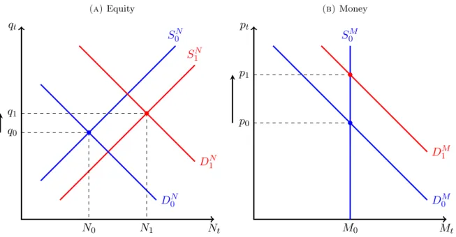
Money market. Figure2B illustrates the immediate effects of the shock on the money mar-ket. Demand comes from entrepreneurs and supply is fully controlled by the government. D0M and S0M are the initial (i.e. steady state) demand and supply curves, respectively. Savers in-crease their demand for money after net worth improvements; this is illustrated by a rightward
Figure 2: Asset markets and immediate effects of the tax shock (a)Equity Nt qt S0N S1N DN0 DN1 q0 N0 q1 N1 (b)Money Mt pt S0M M0 D0M D1M p0 p1
NOTES:Ddenotes demand andSdenotes supply. SuperscriptsNandM denote equity and money, respectively. Subscripts 0 and 1 denote steady state and quarter 1, respectively.
shift of D0M toDM1 . With exogenously fixed money supply, the result is a higher price.
Equity market. Figure 2A illustrates immediate effects of the shock on the equity market. DN0 and S0N are the initial (steady state) demand and supply curves, respectively. Demand comes from savers and the government; supply comes from investors. Savers increase their demand for equity following net worth improvements; this is illustrated by a rightward shift of DN0 toDN1 . Equity’s supply increases as investors issue new issues to finance their investment; this is represented by a rightward shift of S0N toS1N. The increase in supply is small; because of the borrowing constraint, investors issue a small amount of equity relative to the additional investment cost. As a consequence, equity’s market price increases.
Internal amplification. A demand for money exists because of both liquidity constraints; the borrowing constraint, in particular, restricts the shock-induced increase in equity supply to be small, and is therefore responsible for the asset’s higher price. Increases in both asset prices amplify the net worth improvements of entrepreneurs, which in turn increases asset demand and investment. This “internal amplification” mechanism originates from the liquidity constraints and is the cause of the long-term persistence of the shock.
Consider a counterfactual scenario. If the borrowing constraint is calibrated sufficiently loose then the shock encourages investors to issue a considerable amount of new equity, and (as if S1N is further to the right than drawn in Figure 2A) the shock then reduces the price of the asset. This result implies a higher expected return on equity, which encourages agents to substitute away from money. Depending on the relative sizes of this portfolio balance effect and the positive wealth effect, money’s price either increases by a smaller degree than in the baseline calibration or decreases altogether. If the latter result holds, i.e. both asset prices
fall, then the ceteris paribus effects on entrepreneurs from the cut in the dividend tax rate are (partially or completely) offset. In particular, a first quarter increase in investment is not achieved. Without an increase in investment, aggregate demand decreases. And, as explained in Section3.2, investment is key to the internal propagation of the shock, particularly for output.
Private consumption. Aggregate private consumption’s largest contributor comes from workers. The fall in the real wage is larger than the rise in employment (see Table 1), and therefore the aggregate gross wage decreases. But because of the drop in the tax rate, workers enjoy a higher aggregate net wage and, being non-Ricardian, consume more general output. Savers and investors consume more because of improvements in the net worth. Accordingly, total consumption increases.
Government. The cuts to wage and dividend income tax rates are equivalent to 1% and 2.8% of national output, respectively. Tax collections fall by 3.3% ceteris paribus.11 With more output and a smaller aggregate gross wage bill, the aggregate gross dividends to capital are higher (from Equation (2.50)). These endogenous changes in tax bases together with the tax rate cuts cause tax collections to fall by 3.1% (from Equation (2.12)). The government holds no stocks of money and equity, and is therefore unaffected by asset price changes. The fiscal budget is balanced by matching the decrease in taxation with a reduction in government spending. However, the strong increase in investment together with the increase in private consumption outweigh the decrease in government spending.
3.2 Path to adjustment
The speed of convergence is indicated by the time a variable takes to get “close” to steady state. A variable is considered “close” to steady state if the percentage deviation is within 10% of the immediate shock response. The last column of Table1gives this indicator convergence. Table1
also gives the largest impulse response by magnitude and the quarter in which this occurs. The model’s calibration assumes that, from the second quarter, the shock deteriorates at an assumed rate of 5% per quarter, and both tax rates asymptotically increase towards their steady state levels. As the effects of the shock ware off, asset prices and private consumption converge steadily towards steady state.
The steady state level of investment creates a quantity of new capital that exactly replaces depreciated units. Since the shock increases investment above its steady state level, the capital stock increases by the end of the first quarter. In the second quarter, as tax rates start increasing towards pre-shock levels, workers reduce their labour supply; in the labour market, this produces an increase in the real wage and a decrease in employment. Long-term economic growth is thus achieved by increases in the capital stock. This is why investment is described as the “internal propagation” mechanism.
Furthermore, with more output and a lower aggregate wage bill, gross aggregate dividends are higher. This in part helps entrepreneurs enjoy higher-than-normal net worth. Investment is therefore sustained above steady state, and the capital stock continues to increase. The stock
11
peaks after almost 9 years at 23.6% above steady state. By then, the level of depreciation starts to exceed investment, and the capital stock starts to return to its pre-shock level. This is why capital exhibits a hump-shaped trajectory.
Employment persistently declines since its initial response to the shock. Workers continue with their supply reduction in response to the increase in the rate of tax. The real wage increases, and even overshoots its steady state level in the 10th quarter. It peaks just after 11 years at 0.9% above steady state (after falling below by 0.9% in the first quarter). The eventual decline in the wage rate occurs when entrepreneurs reduce their labour demand when the capital stock starts decreasing.
Output remains heavily influenced by capital, and even traces the same hump-shaped tra-jectory. Over its adjustment path, output is kept elevated above its steady state level while it converges. It increases continuously for almost 7 years before returning towards its pre-shock level. But the return is slow, and even after 200 quarters it is still approximately 0.2% above steady state, after being 1.8% above at its peak.
4
Tax multipliers
The objective of this section is to describe the shock responses in Section3as either “large” or “small”. To do this, responses are quantified by tax multipliers. A variable’s response is then described as “large” if the absolute value of its tax multiplier is in excess of unity; otherwise the response is “small”. Multipliers are more suitable than impulse responses for describing the magnitude of the effects of the shock, for two reasons. Firstly, the shock is not normalized, because of its duality, and impulse responses are therefore difficult to interpret on their own. Multipliers, on the other hand, measure normalized responses. Secondly, these multipliers are constructed to measure the fall in tax collections due to cuts in both tax rates,ceteris paribus. They therefore disentangle the discretionary change in taxes (i.e. the change in tax rates) from the endogenous component (i.e. the changes in tax bases, wtLt and rtKt).12 Multipliers are
computed according to the methodology outlined below, and results are given in Table2. This section omits any further multiplier analysis of the tax shock, because it would say the same things as the impulse responses analysis in Section3.
4.1 Methodology
Tax multipliers are obtained for real aggregate variables only. Impact and cumulative multipliers are calculated. Changes in both tax rates are captured by a single variable,Tt∗, which represents government tax collections with tax bases held constant to their steady state levels, i.e. from Equation (2.12),
Tt∗=τtrnrN+τtwlwL (4.1) where notation without time subscripts represent steady state (i.e. t = 0) values. Changes in Tt∗ therefore representceteris paribus changes in taxes. The deviation of taxes in period tfrom
12
Perotti (2012) highlights the importance of separating discretionary from endogenous changes in taxes by showing they have different effects on output.
steady state with tax bases held constant is
Tt∗−T = (τtrn−τrn)rN + (τtwl−τwl)wL (4.2) If the immediate post-shock tax rates are τ1rn and τ1wl then the immediate change in Tt∗ is
T1∗−T = (τ1rn−τrn)rN + (τ1wl−τwl)wL (4.3) Tax multipliers therefore measure the response of a variable, over a given period of time, to a drop in government tax receipts by 1 unit of general output due to discretionary cuts in both tax rates,ceteris paribus.
Impact multipliers measure the response of a real aggregate variable in periodtto the change inTt∗ in period 1,
Xt−X
T1∗−T (4.4)
Of special interest in this class of multipliers is the period 1 response of the variable, or the immediate impact multiplier,
X1−X
T1∗−T (4.5)
Cumulative multipliers measure the variable’s response over a period of time. They capture accumulated changes in the variable as well as accumulated changes in the policy variable. Cumulative tax multipliers are measured over 0.5, 1, 2, 3, and 4 year horizons according to
Pn
t=1(Xt−X)
Pn
t=1(Tt∗−T)
(4.6)
4.2 Results: multiplier responses
Multipliers measure the change in a real variable, i.e. in terms of units of output, for every unit of general output that the government gives up in tax revenue in the first quarter, due to discretionary cuts in both tax ratesceteris paribus. A negative (positive, respectively) multiplier indicates that the variable increases (decreases, respectively) after the shock. If cumulative multipliers of a variable increase (decrease, respectively) with the measured time horizon, then the variable is converging slower (faster, respectively) than Tt∗ towards steady state.
Output and private consumption have very large, negative responses to the shock, both contemporaneously and cumulatively. On impact, output and consumption increase by 2.9 and 3.5 units of general output, respectively, for every unit the government gives up from tax cuts, ceteris paribus. Both their cumulative multipliers increase with the time horizon. This suggests that while the shock itself wares off, its effects on output and consumption continue to propagate. It also confirms the slow convergence that is suggested graphically by Figure 1. Investment has a moderate increase. A unitary multiplier is observed on impact of the shock, and as the shock wares off, investment converges at a uniformly proportional and slightly slower rate than Tt∗.
By far, the largest responses are by asset prices. They both increase substantially, with impact multipliers of –11.8 for money and –5.3 for equity, and with similar values cumulatively
Table 2: Multipliers of a tax shock: baseline scenario
Immediate impact
Cumulative
6-month 1-year 2-year 3-year 4-year
Yt −2.9 −3.1 −3.4 −4.2 −4.9 −5.7 It −1.0 −1.1 −1.1 −1.1 −1.1 −1.1 Ct −3.5 −3.6 −3.7 −4.0 −4.2 −4.5 Ctw −2.1 −2.1 −2.2 −2.3 −2.5 −2.7 Cti 0.0 0.0 0.0 0.0 0.0 0.0 Cts −0.2 −0.2 −0.2 −0.2 −0.2 −0.2 wt 3.1 3.0 2.7 2.1 1.5 0.9 rt 0.0 0.0 0.0 0.0 0.0 0.0 pt −11.8 −11.8 −11.8 −11.9 −11.9 −11.9 qt −5.3 −5.2 −5.2 −5.2 −5.1 −5.0
NOTES: This table shows the multiplier responses to exogenous cuts in tax rates,ceteris paribus. Responses are measured relative to the drop in overall tax collections while holding tax bases constant. For every 1 unit less of general output the government collects in tax revenue in the first quarter, multipliers measure the consequential changes in endogenous variables. A negative multiplier indicates that the variable increases after the drop in taxes.
over the various measurement horizons. Both contemporaneously and cumulatively, savers’ consumption has a small increase (with multipliers of –0.2), and investors’ consumption and the rate of return on capital have insignificant responses (with multipliers near 0).
5
Sensitivity analysis
The robustness of results is examined with respect to the calibration of structural parameters and the persistence of tax shocks. For brevity, the details and results of these exercises are provided in Appendix B. The overall conclusion is that results are qualitatively robust, but quantitatively sensitive, to assumptions regarding structural parameter values, and qualitatively and quantitatively sensitive to significant variations in the persistence of tax shocks.
5.1 Sensitivity to structural parameters.
Structural parameter sensitivity analysis is performed systematically by three local methods, all involving repeated simulations of the shock with combinations of sensitivity settings that are listed in Table 4. The first method uses one change in one parameter at a time; the second and third methods use combinations of two or more sensitivity parameter values. Results are quantitatively sensitive to one-at-a-time variation of three structural parameters: the subjective discount factor (β), capital’s share in output (γ), and the survival rate of capital after depreci-ation (δ). The model is also sensitive to combinations of alternative parameter settings, more so when these settings go beyond those of β,γ, and δ. Nevertheless, from changing parameter values either one-at-a-time or in combinations, tax shock responses vary only in magnitude, and
not in direction or adjustment trajectories. Finally, comparing baseline responses to alternatives from all possible combinations of parameter values shows that, with the exception of investors’ consumption,Cti, baseline responses are not extreme.
5.2 Sensitivity to the persistence of tax shocks.
Sensitivity to the persistence of tax shocks,ρτ wl andρτ rn, is examined by repeatedly simulating
the shock with simultaneous use of values above and below the calibrated (and fairly standard) setting. Results are quantitatively and qualitatively sensitive to the calibration of the persistence parameters for tax shocks,ρτ rn andρτ wl. Very small changes in the persistence parameters do
very little to alter responses; but with larger parameter variations there are significant changes in trajectory and convergence. Lowering the level of persistence reveals that investment, savers’ equity, capital, investors’ consumption, and output are still slow to converge to steady state. This suggests that features in the model – in particular, the liquidity constraints – are responsible for their long-term responses the shock. The mechanism, called the “internal amplification” mechanism, is described in the analysis of the shock.
6
Discussion
6.1 Comparison of results
This paper is closely related toMountford and Uhlig (2009) (henceforth MU), who show that an unexpected, exogenous increase in government spending that is completely financed by an increase in taxation causes reductions in private consumption and investment on impact, as well as in output from the second period.13 The converse of this result suggests a recipe for debt-free economic expansion. This paper complements MU by showing that the converse of their result is also true. The novelty of this paper is that while MU obtain their results from an empirical study with vector autoregressions, this paper is a theoretical investigation using a mostly neoclassical DSGE model.
Eggertsson (2010) also propose a balanced budget stimulus with tax rate cuts. He uses a New Keynesian model with sticky prices and monopolistic competition, and compares the effects of cutting different tax rates. His recipe, therefore, is to cut consumption taxes and raise wage income and wealth taxes. However, he also suggests that liquidity constraints may reverse the intended responses. Conclusions between this paper and Eggertsson (2010) are different because this paper does not feature consumption taxes or New Keynesian frictions.
Romer and Romer (2010), Mertens and Ravn (2011a,b, 2012), and Monacelli et al. (2012) estimate vector autoregressions using, as the basis of datasets, the narrative record of exogenous US fiscal shocks developed by Romer and Romer (2010). These papers explore and quantify the macroeconomic effects of changes in taxation. Their peak cumulative multipliers are given in Table3.14 Despite the differences in methodology, these papers arrive at the same conclusion as this paper, i.e. they support fiscal expansion by tax reductions. Estimated multipliers for output, consumption, and investment are large and negative, and responses exhibit long-term
13
There is, however, a small increase in output on impact, with a multiplier of 1.3.
14
Table 3: Multipliers: a survey
Output Consumption Investment Employment
Romer and Romer (2010) –2.9 (10 quarters)
Mertens and Ravn(2011a) –2.0 –2.0 –10.0 –1.0
(10 quarters) (10 quarters) (10 quarters) (10 quarters)
Mertens and Ravn(2012) –1.8 (3 quarters)
Monacelli et al. (2012) –2.7 –9.7 –0.5
(1 year) (1 year) (2 quarters)
NOTES: This table gives the peak cumulative multipliers from a 1% cut in taxation, and (in brackets) the time after the shock these multipliers are observed. A negative multiplier therefore represents an increase in the variable.
persistence. However, their results suggest weaker output and consumption responses and a much stronger investment response than the ones found here.
6.2 Relationship with the KM-related literature
The 2007/8 financial turmoil brought a wave of recent attention toKiyotaki and Moore(2012), for two reasons. First, commentators argue that the cause of the crisis was the sudden and unex-pected deterioration in the value of partially liquid private financial assets (Brunnermeier(2009),
Del Negro et al.(2011), Bigio (2012) and Jermann and Quadrini(2012)). Assets’ resaleability and collateral suitability were thus adversely affected. This event bears a striking resemblance to KM’s negative liquidity shock. Secondly, the government holding risky, privately-issued as-sets with limited resaleability was the central component of the unconventional policy responses to the crisis, whereby these assets were exchanged for safe, liquid, government-issued securities and cash.15 This is, in fact, KM’s main policy implication, that government can inject liquidity to counter-cyclically dampen business cycle fluctuations.
The KM model is theoretically adjusted and/or extended in a series of recent papers. These papers can be classified into two groups. The first group uses the KM model to evaluate the unconventional policies seen in the crisis; Del Negro et al.(2011) andDriffill and Miller(2013) are members of this research, and both show that recessions would have been exacerbated had it not been for government interventions. The second KM-related group returns to the original questions posed by KM on the importance of (i) liquidity shocks for explaining business cycles, and (ii) liquidity constraints for the propagation of productivity shocks. Papers in this group includeSalas-Landeau(2010),Bigio(2010,2012),Ajello(2011),Nezafat and Slav´ık(2012),Shi
(2012), andJermann and Quadrini (2012).
The inclusion of distortionary taxes and a balanced budget rule is not unique in KM-related literature. Ajello (2011), Shi (2012), and Driffill and Miller (2013) have a balanced budget
15
The various facilities through which the US government implemented these exchanges are described in Ar-mantier et al.(2008),Fleming et al.(2009),Adrian et al.(2009), andAdrian et al.(2011).
rule for government. Ajello (2011) also includes distortionary taxes, but he modifies the KM model more extensively than in this paper. The uniqueness of this contribution is that it is the first to examine fiscal shocks in the KM model. What is shares with these papers, the second KM-related group in particular, is showing the macroeconomic significance of KM’s liquidity constraints in propagating exogenous shocks. In this case, however, the shocks are to tax rates.
6.3 The significance to New Keynesian frictions
One significance of this paper is that it shows how a neoclassical model can be modified to produce large responses to fiscal shocks. The New Keynesian model is the workhorse for fiscal policy research. This perhaps follows from papers likeBurnside et al.(2004), which shows that the magnitude of observed responses to fiscal shocks are not matched by a standard neoclassical models, but they are matched by models that include habit formation and adjustment costs. Beyond the liquidity constraints, this model is otherwise neoclassical. This paper therefore shows that a host of New Keynesian frictions are not always needed to study fiscal policy. The KM model can be a workhorse for that purpose.
7
Conclusion
This paper shows that cuts to income tax rates in a liquidity constrained economy increases output, investment, and private consumption. The model is a modification of the mostly neo-classical, DSGE model of liquidity and business cycles by Kiyotaki and Moore (2012). In particular, distortionary taxes and a balanced budget fiscal rule are added to KM. The model is calibrated to be consistent with the KM-related literature. Results are qualitatively robust, but quantitatively sensitive, to assumptions regarding structural parameter values, and qualitatively and quantitatively sensitive to significant variations in the persistence of tax shocks.
This paper is unique in three ways. Firstly, these results are consistent with those obtained byMountford and Uhlig(2009); but while they use an estimated VAR, this paper complements and supports with a theoretical finding from a calibrated neoclassical model. Secondly, this paper distinguishes itself from the rest of the KM-related literature by being the first to apply the KM model to fiscal shocks; this related literature remains focused on showing the significance of liquidity shocks in explaining business cycles, and the importance of liquidity constraints for propagating productivity shocks. Thirdly, the paper shows how a neoclassical model can be modified to produce large responses to fiscal shocks.
Some opportunities for future research are suggested by this work. One extension is an examination of a cut in taxes without a balanced budget in this environment. Another useful experiment is to cut one tax rate at a time, and determine their relative merits in the economic expansion seen in this paper. It would be interesting to determine the effects of an increase in government spending, with and without a balanced budget. The model can be adjusted by adding New Keynesian type frictions, and then determine whether such frictions change the results. Finally, taking this study to the data will facilitate the calculation of multipliers that are reliable for quantitatively comparing results with the related literature.