SURFACE
SURFACE
Dissertations - ALL SURFACE
August 2017
Risk-aware navigation for UAV digital data collection
Risk-aware navigation for UAV digital data collection
Zhi XingSyracuse University
Follow this and additional works at: https://surface.syr.edu/etd Part of the Engineering Commons
Recommended Citation Recommended Citation
Xing, Zhi, "Risk-aware navigation for UAV digital data collection" (2017). Dissertations - ALL. 776. https://surface.syr.edu/etd/776
This Dissertation is brought to you for free and open access by the SURFACE at SURFACE. It has been accepted for inclusion in Dissertations - ALL by an authorized administrator of SURFACE. For more information, please contact
This thesis studies the navigation task for autonomous UAVs to collect digital data in a risky environment. Three problem formulations are proposed according to different real-world situations. First, we focus on uniform probabilistic risk and assume UAV has unlimited amount of energy. With these assumptions, we provide the graph-based Data-collecting Robot Problem (DRP) model, and propose
heuristic planning solutions that consist of a clustering step and a tour building step. Experiments show our methods provide high-quality solutions with high expected reward. Second, we investigate non-uniform probabilistic risk and limited energy capacity of UAV. We present the Data-collection Problem (DCP) to model the task. DCP is a grid-based Markov decision process, and we utilize reinforcement learning with a deep Ensemble Navigation Network (ENN) to tackle the problem. Given four simple navigation algorithms and some additional heuristic information, ENN is able to find improved solutions. Finally, we consider the risk in the form of an opponent and limited energy capacity of UAV, for which we resort to the
Data-collection Game (DCG) model. DCG is a grid-based two-player stochastic game where the opponent may have different strategies. We propose opponent modeling to improve data-collection efficiency, design four deep neural networks that model the opponent’s behavior at different levels, and empirically prove that explicit opponent modeling with a dedicated network provides superior performance.
by Zhi Xing
B.S., Nankai University, 2010 M.S., Syracuse University, 2017
Dissertation
Submitted in partial fulfillment of the requirements for the degree of Doctor of Philosophy in Computer and Information Science and Engineering.
Syracuse University August 2017
I’m extremely grateful to my advisor Professor Jae C. Oh, who changed my life by giving me the opportunity to study in the program. During my study, Professor Oh, as a mentor and a friend, provided me the most wonderful guidance beyond doing research. Looking back after all these years, one of the things I appreciate the most is the complete research freedom he granted me. Admittedly, it was
challenging at the beginning. But as time goes by, I’ve learned how to explore in addition to how to exploit, how to give in addition to how to receive, and how to lead in addition to how to follow. I’ve grown so much as Professor Oh’s advisee that I’m well prepared to face any future challenges.
I want to thank my family – my wife, Yuchen Deng, parents, Hongxia Xu and Jinshu Xing, and parents-in-law, Guifang Xu and Hong Deng – for their
unconditional trust and support throughout the years. Their love gives me the strength and courage to do what I want to.
Last but not least, I want to thank my committee members Professor Young B. Moon, Professor Chilukuri Mohan, Professor Qinru Qiu, Professor Sucheta
Soundarajan and Professor Jian Tang. Their insights and suggestions have greatly enriched my work.
Page ABSTRACT . . . i LIST OF TABLES . . . ix LIST OF FIGURES . . . xi 1 Introduction . . . 1 1.1 Motivation . . . 1 1.2 Problem framework . . . 2 1.3 Thesis overview . . . 3 2 Background . . . 6 2.1 Hierarchical Clustering . . . 6
2.2 Rooted k Minimum Spanning Tree . . . 8
2.3 Convolutional Neural Network . . . 8
2.4 Markov Decision Process and Stochastic Game . . . 11
2.5 Reinforcement Learning . . . 12
2.5.1 Q-learning . . . 13
2.5.2 Policy gradient . . . 13
2.5.3 Deep Reinforcement Learning . . . 14
2.6 Opponent modeling . . . 16
3 Graph formulation with uniform risk . . . 19
3.1 Chapter overview . . . 19
3.2 Contributions . . . 20
3.3 Problem formulation . . . 20
3.4 Algorithm . . . 22
3.4.1 Clustering for the number of robots . . . 22
3.4.2 Heuristics for building tours . . . 25 vi
3.4.3 The Progressive Gain-aware Clustering algorithm . . . 29
3.5 Evaluation . . . 32
3.5.1 Comparison of tour-building algorithms . . . 34
3.5.2 Comparison of clustering algorithms . . . 35
3.5.3 Effect of node reward variance . . . 36
3.6 Related work . . . 37
3.7 Conclusion . . . 39
4 Grid formulation with non-uniform risk and energy constraint . . . 45
4.1 Chapter overview . . . 45
4.2 Contributions . . . 46
4.3 Problem formulation . . . 47
4.4 Algorithm . . . 49
4.4.1 Maximizing reward without energy constraint . . . 49
4.4.2 Navigation under energy constraint . . . 52
4.4.3 Finding the balance. . . 55
4.5 Evalution . . . 60
4.5.1 Different risk distributions . . . 63
4.5.2 Effect of reward density . . . 65
4.5.3 Effect of energy capacity . . . 67
4.5.4 Single-item data collection . . . 68
4.5.5 Comparison to other learning methods . . . 71
4.6 Related work . . . 72
4.7 Conclusion . . . 73
5 Grid formulation with opponent and energy constraint . . . 75
5.1 Chapter overview . . . 75 5.2 Contributions . . . 76 5.3 Problem formulation . . . 78 5.4 Algorithm . . . 80 5.4.1 State representation . . . 80 vii
5.4.2 No Opponent Modeling. . . 80
5.4.3 Implicit Opponent Modeling . . . 82
5.4.4 Explicit Opponent Modeling with same network . . . 83
5.4.5 Explicit Opponent Modeling with separate network . . . 85
5.4.6 Comparison of the networks . . . 86
5.5 Evaluation . . . 87
5.5.1 Environmental settings . . . 88
5.5.2 Network structure and hyperparameters . . . 89
5.5.3 Evaluation in the standard setting. . . 89
5.5.4 Effect of energy capacity . . . 92
5.5.5 Investigation on the behaviors . . . 95
5.5.6 Five million steps of training . . . 104
5.5.7 Change of opponent strategy. . . 109
5.6 Related work . . . 110
5.7 Conclusion . . . 111
6 Summary and future work . . . 113
LIST OF REFERENCES . . . 115
VITA . . . 118
Table Page 3.1 Overview of tour-building algorithms. Criterionsummarizes the what is
evaluated by each algorithm. Insertion positionspecifies where does an algorithm insert a new node. Time complexityshows the computational complexity of an algorithm. . . 25 4.1 Results of experiments on the tour-building heuristics from Chapter 3
adopted to DCP. The average is taken from 10,000 runs. For every run, there is one agent with infinite amount of energy, the total reward is 30, and the risk distribution is as Figure 4.1b. Reward Avg. is the average of total reward collected during a game. Reward SD. is the standard deviation. . . 50 4.2 Risk values of the three different risk distributions used in Section 4.5.1.
Each distribution has four layers of risk values. From outer to inner, the risk values are ρ(0), ρ(1), ρ(2) and ρ(3). As an example, high risk is shown in Figure 4.1b. . . 61 4.3 Results of experiments on the high-risk distribution specified in Table 4.2.
The average is taken from 10,000 runs. For every run, the total reward is 30, and the initial and maximal energy of agent is 8 and 16 respectively.
Rewardis the total reward collected during a game. Energyis the total energy consumed during a game. Reward / Energy is the reward col-lected per energy consumed during a game. Avg. means the average over 10,000 runs. SD. is the standard deviation. Incr.% is ENN’s increment as a percentage of an algorithm’s corresponding average. For example, Safe-Reward’s reward incr.% is the difference between ENN’s reward and Safe-Reward’s reward as a percentage of Safe-Reward’s. . . 62 4.4 Results of experiments on the medium-risk distribution specified in
Ta-ble 4.2. Terms used in the taTa-ble and other experimental settings are the same as Table 4.3. . . 62 4.5 Results of experiments on the low-risk distribution specified in Table 4.2.
Terms used in the table and other experimental settings are the same as Table 4.3. . . 62 4.6 Results of experiments where the total reward is 15. Terms used in the
table and other experimental settings are the same as Table 4.3. . . 66
4.7 Results of experiments where the initial and maximum energy levels are set to 16 and 32 respectively. Terms used in the table and other experimental settings are the same as Table 4.3. . . 67 4.8 Results of experiments where there is only one item of reward one in the
environment. Terms used in the table and other experimental settings are the same as Table 4.3. . . 68 4.9 Results of experiments for a simple linear learner. Terms used in the table
and other experimental settings are the same as Table 4.3. . . 69 4.10 Results of experiments for the EQN shown in Figure 4.4. Terms used in
the table and other experimental settings are the same as Table 4.3. . . 69
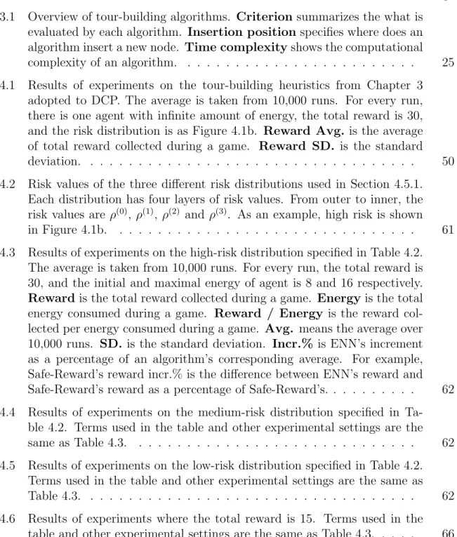
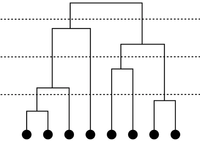
Figure Page 2.1 An example dendrogram from Hierarchical Clustering of 8 elements. The
black dots represent elements. The solid lines indicate merges or splits. The dotted lines show different positions for cuts. In top-down order, the cuts result in 2, 4 and 6 clusters. . . 7 2.2 An example of a convolutional layer with input and outputs. The input is
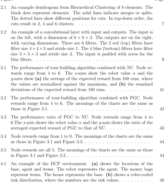
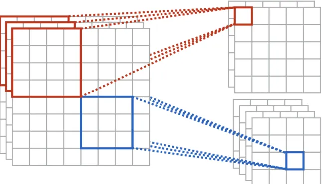
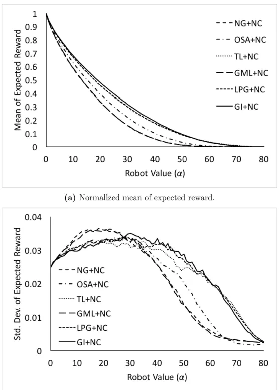
on the left, with a dimension of 8×8×3. The outputs are on the right, with varying dimensions. There are 6 filters. The 2 red (top) filters have filter size 4×4×3 and stride size 1. The 4 blue (bottom) filters have filter size 3×3×3 and stride size 2. The input is padded with zeros for the blue filters. . . 9 3.1 The performance of tour-building algorithm combined with NC. Node
re-wards range from 4 to 6. The x-axes show the robot value α and the
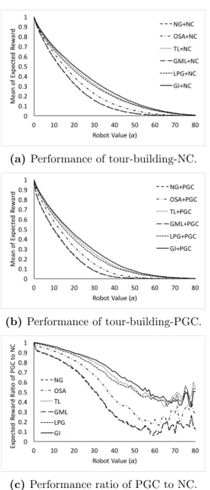
y-axes show (a) the average of the expected reward from 100 runs, where the values are normalized against the maximum, and (b) the standard deviations of the expected reward from 100 runs. . . 41 3.2 The performance of tour-building algorithm combined with PGC. Node
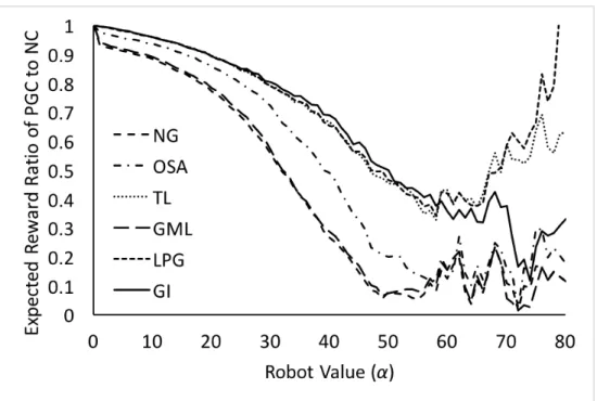
rewards range from 4 to 6. The meanings of the charts are the same as those in Figure 3.1. . . 42 3.3 The performance ratio of PGC to NC. Node rewards range from 4 to
6.The x-axis shows the robot valueα and they-axis shows the ratio of the averaged expected reward of PGC to that of NC. . . 43 3.4 Node rewards range from 1 to 9. The meanings of the charts are the same
as those in Figure 3.1 and Figure 3.3. . . 44 3.5 Node rewards are all 5. The meanings of the charts are the same as those
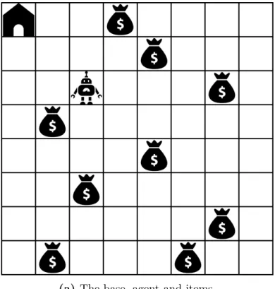
in Figure 3.1 and Figure 3.3. . . 44 4.1 An example of the DCP environment. (a) shows the locations of the
base, agent and items. The robot represents the agent. The money bags represent items. The house represents the base. (b) shows a color-coded risk distribution, where the numbers are the risk values. . . 48
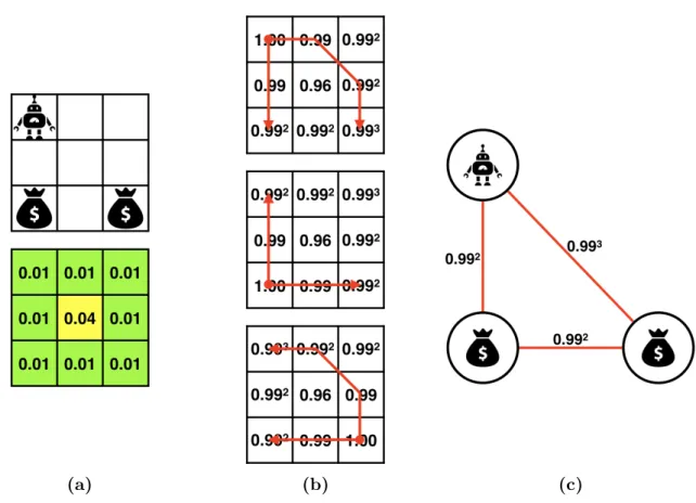
4.2 Extracing a complete undirected graph from a game state. (a) shows the original game state. The bottom grid contains risk values. (b) shows the safest paths calculated by Dijkstra’s Algorithm for (from top down) the agent, the left item and the right item. The numbers are success probabilities instead of risk values. (c) shows the complete undirected graph created from the safest paths. The nodes represent the agent and items, and the edge weights are the success probabilities of safest paths. 50 4.3 Structure of ENN. ENN is composed of a Convolultional Neural Network
(CNN) and a number of heuristics Hi, all of which take game state s as
input. The heuristics output action vectors Hi(s) and the CNN outputs
one weight wi(s;θ) for each action vector, a bias b(s;θ), and a state value
estimation V(s;θv), where θ and θv represent network parameters. The
final policy π(s;θ) is a softmax function σ of a linear combination of all the outputs. . . 56 4.4 Structure of EQN. EQN is composed of a Convolultional Neural Network
(CNN) and a number of heuristicsHi, all of which take game statesas
in-put. The heuristics output action vectors Hi(s) and the CNN outputs one
weightwi(s;θ) for each action vector and a biasb(s;θ), whereθrepresents network parameters. The final output is an estimate of the state-action value function Q(s, a;θ) for every action a, which is a linear combination of all the heuristic outputs. . . 70 5.1 An example of the DCG environment. The robot represents the collector.
The ghost represents the adversary. The money bags represent items. The house represents the base. . . 77 5.2 Structure of VNN in Section 5.4.2. VNN is a Convolultional Neural
Net-work. It takes statesas input, and gives the policyπ(s, h;θ) and the value estimationV(s, h;θv) as outputs, whereθand θv are network parameters. 81
5.3 Structure of IMNN in Section 5.4.3. IMNN is a Convolultional Neural Network. It takes state s and history h as inputs, and gives the policy
π(s, h;θ) and the value estimation V(s, h;θv) as outputs, where θ and θv
are network parameters. . . 82 5.4 Structure of EMNN in Section 5.4.4. EMNN is a Convolultional
Neu-ral Network. It takes state s and history h as inputs, and gives the policy π(s, h;θ), the value estimation V(s, h;θv), and opponent strategy
πo(s, h;θ
o) as outputs, where θ, θv and θo are network parameters. . . . 83
Convolultional Neural Networks. OMN takes state s and history h as inputs, and gives the opponent strategy πo(s, h;θo) as output. CoNN
takes state s, history h, and opponent strategyπo as inputs, and gives the policy π(s, h, πo;θ) and the value estimation V(s, h, πo;θ
v) as outputs. θ, θv and θo are network parameters. . . 85
5.6 Results on episode reward for networks trained in 1 million steps. The labeled bars in the chart show the averaged episode rewards over 10,000 episodes. The error bars are the standard deviations. . . 90 5.7 Results on reward per energy (RPE) for networks trained in 1 million
steps. The labeled bars in the chart show the averaged RPEs over 10,000 episodes. The error bars are the standard deviations. . . 90 5.8 Results on episode reward for different maximum energy levels. The
la-beled bars in the chart show the averaged episode rewards over 10,000 episodes. The error bars show the standard deviations. . . 92 5.9 Results on reward per energy (RPE) for different maximum energy levels.
The labeled bars in the chart show the averaged RPE over 10,000 episodes. The error bars show the standard deviations.. . . 93 5.10 Reward areas of different sizes. The sizes are defined by the edge length
in terms of the number of cells in the square. For a given reward area, one item of reward one is uniformly randomly placed in a cell within the square. . . 95 5.11 Results on episode reward for different sizes of reward area. The labeled
bars in the chart show the averaged episode rewards over 10,000 episodes. The error bars show the standard deviations. In each episode, there is only 1 item of reward 1, and it is randomly placed in a square to the bottom-right of the grid. The size of reward area indicates the edge length of the square. . . 96 5.12 Results on reward per energy (RPE) for different sizes of reward area. The
labeled bars in the chart show the averaged RPE over 10,000 episodes. The error bars show the standard deviations. In each episode, there is only 1 item of reward 1, and it is randomly placed in a square to the bottom-right of the grid. The size of reward area indicates the edge length of the square. . . 97
5.13 Gameplays of VNN and OMN + CoNN when the opponent uses the pa-trol strategy. The robot represents the collector, the ghost represents the opponent, and the money bag represents the item. The base and the en-ergy level of the collector are not shown. The reward of the item is one. The numbers under the grids show the time steps, and the number on the top and left edges of the first grid are the coordinates of the grid cells. The three big dots between grids indicate omitted steps, while those at the end indicates infinite number of steps. . . 100 5.14 Gameplays of VNN and OMN + CoNN when the opponent uses the
re-strictedstrategy. The robot represents the collector, the ghost represents the opponent, and the money bag represents the item. The base and the energy level of the collector are not shown. The reward of the item is one. The numbers under the grids show the time steps, and the number on the top and left edges of the first grid are the coordinates of the grid cells. The three big dots between grids indicate omitted steps, while those at the end indicates infinite number of steps. . . 101 5.15 Gameplays of VNN and OMN + CoNN when the opponent uses the
with-fog strategy. The robot represents the collector, the ghost represents the opponent, and the money bag represents the item. The base and the energy level of the collector are not shown. The reward of the item is one. The numbers under the grids show the time steps, and the number on the top and left edges of the first grid are the coordinates of the grid cells. The three big dots between grids indicate omitted steps. . . 102 5.16 Results on episode reward for networks trained in 5 million steps. The
labeled bars in the chart show the averaged episode rewards over 10,000 episodes. The error bars are the standard deviations. . . 104 5.17 Results on reward per energy (RPE) for networks trained in 5 million
steps. The labeled bars in the chart show the averaged RPEs over 10,000 episodes. The error bars are the standard deviations. . . 105 5.18 Results on episode reward for networks trained in 1 million steps. The
labeled bars in the chart show the averaged episode rewards over 10,000 episodes. The error bars are the standard deviations. Thewith-fog strat-egy is replaced by the double-blind with-fogstrategy where agents can-not see each other when the collector goes into special “foggy” cells. . . 107 5.19 Results on reward per energy (RPE) for networks trained in 1 million
steps. The labeled bars in the chart show the averaged RPEs over 10,000 episodes. The error bars are the standard deviations. Thewith-fog strat-egy is replaced by the double-blind with-fogstrategy where agents can-not see each other when the collector goes into special “foggy” cells. . . 108
1. INTRODUCTION
1.1 Motivation
Robots have been working among humans for many years, on simple and repetitive tasks such as cashier, phone operator and bank teller, or on dangerous tasks such as extraterrestrial explorations. With the advances in areas such as computer vision, machine perception, and control theory, robot’s capabilities and potentials have been greatly increased. As a result, humans are gradually being replaced by robots in more complex tasks as driving, package delivery, and image/video surveillance.
Robots have many advantages over humans. They can vary in sizes to suit the task to be accomplished, they can perform repetitive tasks faster, they can survive in harsh environments, and they usually cost less than human employees. In
addition, they are even more reliable when it comes to tasks that require precision, such as surgery, because they can eliminate human errors. In this thesis, we want to make use of these good traits in the domain of autonomous data collection.
Consider scientific exploration in an uninhabited environment like a rainforest or an island. Scientists need to collect data from different locations periodically. But the environment may be too dangerous for human expedition. It would be too costly and inefficient. Fortunately, the scientists have a lot of expandable UAVs that
are able to collect data and communicate with the satellite.1 The autonomous UAVs are so affordable that even hiring humans to operate them would be more costly than using autonomous agents to control them instead. The scientists can set the locations of interests and let the UAVs collect data autonomously. However, there are threats in the environment that can destroy the UAVs, such as animals and bad weathers, but the autonomous UAVs can select routes efficiently thanks to their state-of-art navigation algorithms. When a UAV is navigated to a location of interest, it can collect data using its various sensors and immediately send the data back to the base station via satellite. Occasionally, UAVs may be destroyed and lost forever, but the algorithms anticipate that and can learn from it. Therefore the goal of the scientists is to collect as much data as possible with a given UAVs. Scenarios like this motivate the work in this thesis.
1.2 Problem framework
As a general framework for the problems studied in this thesis, we consider a data-collection task where autonomous robots are to collect digitaldata. We assume that the robots have communication capability, so they are able to send and receive information. When a robot collects a piece of data, it can immediately send the data to a receiving end, and receives a positive reward amounts to the value of the data. In addition, we assume there are internal (energy) and/or external
(environment, animal, etc.) threats that can disable the robot, after which the robot can no longer move or collect data, and the value of the robot, if there is any, is lost. 1The UAVs are, hopefully, made of environment friendly materials.
We propose three different problem formulations that deal with different real-world scenarios. The problems have different formalism but they share the common goal, which is to maximize the total reward collected from the data with given robots.
1.3 Thesis overview
With the focus on studying the mission of data collection in risky environment, the rest of this thesis is organized as follows.
Chapter 2 provides some theoretical and technical backgrounds for the other chapters. Section 2.1 and 2.2 are applied in Chapter 3. Section 2.3, 2.4 and 2.5 are necessary for both Chapter 4 and Chapter 5. Section 2.6 is utilized by Chapter 5.
Chapter 3 formulates a planning problem on a weighted complete undirected graph. It assumes a known uniform distribution of risk, which is a probability of the robot being disabled, and a unspecified number of robots, and it does not consider energy constraints. This formulation is applicable in cases where finer-grained modeling of risk is impossible or too costly, and the robots have relatively high energy capacity. We propose heuristic algorithms to solve the problem. These heuristic algorithms are able to determine the number of the robots to be deployed and find routes with high expected reward for the robots.
Chapter 4 formulates a Markov Decision Problem (MDP) in a grid-based world. It allows for non-uniform risk, and considers the energy constraints. The risk is also a probability of the robot being disabled. There is only one robot in the MDP and
the robot is able to go back to the base for recharge. This formulation is application in a wider range of cases where the risk distribution is diverse and the energy
capacity of the robot is limited. In such cases, a delicate balance of safety and energy (S&P) needs to be struck, therefore we propose a deep neural network named the Ensemble Navigation Network (ENN) to automatically find this balance.
Chapter 5 formulates a two-player Stochastic Game (SG) in a grid-based world. It also considers energy constraint. However, different from the other two
formulations, the SG does not model probabilistic risk. Instead, the risk is in the form of an opponent. In real-world scenarios, this opponent can model a living entity such as an animal. The robot not only needs to avoid getting disabled by the opponent while collecting data, but also needs to worry about going back to the base for recharge. The focus of Chapter 5 is to use opponent modeling to improve data-collection performance. We propose four deep neural networks that model the opponent in different ways.
We move from graph-based formulation in Chapter 3 to grid formulations in Chapter 4 and 5 due to the following reasons: (1) Although graph is a more general data structure, grid, as a special type of graph, is usually able to model the
real-world reasonably well, which is why it is often the data structure used in video games. (2) Grid can be implemented as array which has much better time and space complexities than graph. (3) Convolutional neural network (CNN), which gained its popularity from the field of computer vision, can be easily applied to grid world by treating each cell as a “pixel”. CNN is able to extract localized features and
Since Chapter 3 belongs to a different field of research than Chapter 4 and Chapter 5, to be consistent with each research community’s convention, we do not
share symbols across chapters, i.e., the same symbol may have different meanings in different chapters. The meaning of symbols are clarified wherever it is necessary. In addition, we use the termsrobot and agent interchangeably, and the terms location of interest and item interchangeably across the proposal. But these terms are used properly to the context of discussions.
Finally, Chapter 6 summarizes all the work presented in this thesis and discusses future directions.
2. BACKGROUND
In this chapter, we provide some of the theories and technologies used in the other chapters. Each section assumes the knowledge of all previous sections. Therefore, if a term is not defined in a certain section, it is defined in the previous ones.
2.1 Hierarchical Clustering
Hierarchical Clustering is a method used to build a hierarchy of clusters. There are two types of Hierarchical Clustering [30]:
• Agglomerative Hierarchical Clustering builds the hierarchy from bottom up. Starting from singletons that consists of a single element, it iteratively merges two clusters into one.
• Divisive Hierarchical Clusteringbuilds the hierarchy from top down. Starting from one cluster containing all the elements, it iteratively splits one cluster into two.
In general, the merges and splits follow some greedy criteria and the resulting hierarchy of clusters is presented in a dendrogram. The dendrogram can be cut at different positions according to different optimization goals, which result in different number of clusters. See Figure 2.1 for an example. In the figure, the black dots represent elements, the solid lines indicate merges or splits, and the dotted lines
Fig. 2.1.: An example dendrogram from Hierarchical Clustering of 8 elements. The black dots represent elements. The solid lines indicate merges or splits. The dotted lines show different positions for cuts. In top-down order, the cuts result in 2, 4 and 6 clusters.
show different positions for cuts. In top-down order, the three cut positions result in 2, 4 and 6 clusters from the same 8 elements.
One of the key characteristics of Hierarchical Clustering is that, unlike more common clustering methods like k-means Clustering, it does not require a
predefined number of clusters. This is useful when the number of clusters should be decided based on the clustering criteria, and this clustering method can
2.2 Rooted k Minimum Spanning Tree
Given a connected undirected graph with weighted edges, a Minimum Spanning Tree (MST) is a subset of the edges that connects all the vertices of the graph, without any cycles, and has the minimum total edge weights. The classical methods for finding the MST include Prim’s algorithm [27] and Kruskal’s algorithm [17], both of which have O(mlogn) time complexity for a graph of m edges and n vertices.
A k-MST, however, asks for a tree of minimum total edge weights that connects exactlyk vertices. When k is a fixed constant, the solution can be found in
polynomial time by trying all the subsets of size k. When k is a variable, the problem is NP-hard [22, 29].
A rooted tree is a tree that consists of a selected vertex, called aroot. A rooted k-MST is therefore a MST that has k vertices, one of which must be the root. Having a root makes Prim’s algorithm easily applicable in finding thek-MST. Starting from the tree that contains only root, the new vertex with minimal-weight edge is added to the tree at each iteration. The process has k−1 iterations, so it is
O(kn) for a graph of n vertices.
2.3 Convolutional Neural Network
Convolutional Neural Networks (CNN) is a bio-inspired feed-forward artificial neural network that has been the key to the recent breakthroughs in Machine Learning [21]. It has been successfully applied to fields including computer vision, speech recognition and natural language processing. Besides these traditional
Fig. 2.2.: An example of a convolutional layer with input and outputs. The input is on the left, with a dimension of 8×8×3. The outputs are on the right, with varying dimensions. There are 6 filters. The 2 red (top) filters have filter size 4×4×3 and stride size 1. The 4 blue (bottom) filters have filter size 3×3×3 and stride size 2. The input is padded with zeros for the blue filters.
supervised learning domains, it is also making aspiring progress in reinforcement learning domains [23, 24, 34]. The key characteristic of CNN is its reduced number of network parameters and its ability to extract different localized features from inputs.
CNN contains one or more convolutional layers, each convolutional layer contains a number of convolutional matrices of parameters, or filters, of different sizes. The size of a filter is usually much smaller than that of the input. Each filter acts as a sliding window over the input matrix. At each step of the sliding, also referred to as a stride, the filter transforms the input submatrix within the window to a single value. This transformation, or convolution, is done at every stride during
the forward pass, and the input matrix is converted to an output matrix of equal or smaller size. Since the same filter is applied at every stride, the number of
parameters is reduced and the network can be deep, which is proven to be crucial for its effectiveness [38].
Figure 2.2 shows an example convolutional layer with input and outputs. The input is on the left, with a dimension of 8×8×3. The outputs are on the right, with varying dimensions. There are 6 filters. The 2 red (top) filters have filter size 4×4×3 and stride size 1. The 4 blue (bottom) filters have filter size 3×3×3 and stride size 2. The input is padded with zeros for the blue filters.
During gradient-descent training, filters can specialize towards different
directions [16]. For example, in the field of computer vision, one filter may specialize in detecting horizontal edges, while another may specialize in detecting vertical edges; one filter may specialize in colors, while another may specialize in contrasts. In other words, different filters are able to extract different localized features from their input.
A convolutional layers is usually followed by a max-pooling layer, which works in a similar way but, instead of convolving with the input, a filter simply picks the highest value within the window. The output of the max-pooling layer is therefore smaller in size than the input, which further reduces the number of network
parameters. At the end, before the output layer, a fully connected layer, as seen in regular neural networks, is normally used for high-level reasoning. This layer summarizes the localized features extracted by the convolutional and max-pooling layers. The summaries are then used for the final output.
2.4 Markov Decision Process and Stochastic Game
Markov Decision Process (MDP) is an extension of Markov Chain. It satisfies the Markov property and provides a framework for modeling decision making in scenarios where the outcome is partially random and partially in the control of the decision maker. It is commonly used to formulate problems that can be solved by dynamic programming or reinforcement learning.
In a standard MDP, an agent interacts with an environment over a number of discrete time steps. At each time stept, the agent receives a statest and selects an
action at from a set of possible actions A according to a policy π, which is a mapping from states st to actions at. After the action is chosen, the environment
transits from the state st to the next state st+1 according to some transition probability function T(st, a, st+1) = P r(st+1|st, at). In return, the agent receives a scalar reward rt. This process repeats until the agent reaches a terminal state, after
which the process restarts. The discounted accumulated return, or returnfor short, is defined as Rt=P∞
k=0γ
krt
+k, where the discounting factor γ ∈[0,1] signifies the
importance of immediate rewards. The goal of the agent is to maximize the return for every state st, in other words, to find the optimal policy π∗.
The generalization of MDP to multiagent case is the Stochastic Game (SG), in which a number of agent interacts with an environment over a number of discrete time steps. At each time step t, each agent z selects an action a(tz) from its own set of possible actions A(z) according to state s
t and its policy π(z). All the actions from
environment transit from st tost+1 according to transition function
T(st,a, st+1) = P r(st+1|st,a). In return, each agentz receives a scalar reward r
(z)
t .
The return for agent z is defined as R(tz)=P∞
k=0γ
kr(z)
t+k and the goal of agentz is to
maximize its own return for every statest by finding its optimal policyπ(z)∗.
If there is no communication between the agents, SG is the same as MDP in the perspective of a particular agent z. In addition, if the other agents use fixed policy, orstrategy, they can be considered as part of the environment and the SG can be reduced to MDP for agent z. But if the other agents use mixed strategy, i.e., their mappings from states to actions may change, the transition function T become unstable for agentz, and it is more difficult for z to find π(z)∗.
2.5 Reinforcement Learning
Reinforcement Learning (RL) is a common method for MDPs and SGs. In RL, the state-action value function Qπ(s, a) =E[Rt|st=s, a] is the expected return for
selecting action a in state s and following policy π afterwards. The optimal value function Q∗(s, a) = maxπQπ(s, a) gives the maximum value achievable for state s
and action a by any policy. Similarly, the state-only value function
Vπ(s) =
E[Rt|st=s] is the expected return of state s for following policyπ. The
advantage function Aπ(s, a) =Qπ(s, a)−Vπ(s) indicates the advantage of actiona
2.5.1 Q-learning
Q-learning is a value-based RL method [35]. It works by learning the optimal value function Q∗(s, a) = maxπQπ(s, a) using the update rule:
Q(st, at)←Q(st, at) +α(rt+γmax at+1
Q(st+1, at+1)−Q(st, at))
where α is the learning rate that decides the strength of each update, and γ is the discounting factor. The values of Q(s, a) is traditionally stored in a table, but can also be in the format of an approximating function if the number of state-action pairs is intractable. When an approximation function is used, the function is
denoted as Q(s, a;θ) withθ representing the parameters of the function. Q-learning is model-free and off-policy, which means it does not learn a model for the
environment and it does not maintain a policy. The policy is implicitly obtained by always choosing action a= arg maxaQ(s, a) ior every states. In practice, an
-greedy strategy, which follows the greedy strategy with probability 1− and selects random action with probability , is often used to ensure adequate exploration of the state space.
2.5.2 Policy gradient
Policy gradient is another common method of RL. It is a policy-based method that optimize a policy approximation functionπ(a|s;θ) directly. In particular, REINFORCE [41] is a policy gradient method that updates function parameterθ in
the direction of∇θlogπ(at|st;θ)Rt. A baseline bt(st) is usually subtracted from the
return Rt to reduce the variance of gradient estimate while keeping the
unbiasedness, giving a gradient direction ∇θlogπ(at|st;θ)(Rt−bt(st)). In practice,
an estimate of the state-only value function V(st;θv) is often used as the baseline,
where θv represents function parameters. This gives us an approximation of the
advantage function A(st, at;θv) =Rt−V(st;θv) where Rt is an estimate of Q(st, at).
The gradient direction then becomes:
∇θlogπ(at|st;θ)A(st, at;θv)
Policy gradient is model-free and on-policy. In an actor-critic policy gradient method, the critic updates the value function parameters, and the actor updates policy parameters according to the gradient suggested by the critic. Compared to a value-based method like Q-learning, the advantages of policy gradient include (1) better convergence properties, (2) effective in high-dimensional or continuous action spaces and (3) can learn stochastic policies. But it typically converge to local rather than global optimum, and evaluating a policy is typically inefficient and has high variance.
2.5.3 Deep Reinforcement Learning
In Deep Reinforcement Learning (DRL), deep neural networks are used as the approximation functions. As a result, DRL brings the benefits of Deep Learning to RL. In particular, the key advantages of DRL methods over traditional RL methods
include (1) its ability to learn from untraceable state space efficiently and (2) its ability to automatically extract features from inputs.
Deep neural network can approximate the state-action value function Q(s, a;θ). In their seminal work [23, 24], Mnih et al. proposed the Deep Q Learning algorithm, which uses a CNN named the Deep Q Network (DQN) asQ(s, a;θ) and achieved professional-human performance on 49 Atari 2600 games. The Q Network learns by taking only raw pixels from the console images and game scores as input. It outputs
Q(s, a;θ) for all the actionsa ∈ A for a given state s. The same network structure works well for all the 49 games, showing a hint of general intelligence. During training, DQN uses a replay buffer to store past experience, which is sampled from for parameter updates. This helps smooth out learning and avoid oscillations or divergence of the parameters.
Many works have been done to improve the performance of DQN. Van Hasselt et al. [39] use Double DQN (D-DQN) to deal with the overestimate problem in
Q-learning. Schaul et al. [33] proposed prioritized experience replay, which uses more important experience more often to improve learning efficiency. Wang et al. [40] employ a dueling network architecture to estimate state value function V(s) and the associated advantage function V(s, a), which are combined to estimate the state-action value function Q(s, a). This architecture is proven to speed up
convergence.
Deep neural network can also approximate the policy function π(a|s;θ) directly. In their following work [25], Mnih et al. proposed Asynchronous Advantage
and theV(s;θv) function. This is an actor-critic method where the policy is the
actor and an estimate of Aπ(s, a) usingV(s;θ
v) is the critic. The CNN used in A3C
learns from the same type of input and shares similar network structure as DQN. A3C uses asynchronous threads to explore state space in parallel to stabilizes training. It runs faster and performs better or equally good with DQN and all the extensions of DQN mentioned above. In addition, A3C is easy to implemented compared with the extensions of DQN, it does not need a replay buffer, and it is able to learn stochastic policies. Therefore, it is chosen as the learning method of our work.
2.6 Opponent modeling
Opponent modeling, or agent modeling in general, is a way to improve a
controlled agent’s performance by identifying and exploiting other agents’ behaviors. In a multiagent environment such as a SG, the environment state st is affected by
the joint action a of all the agents. Let a denote the action of agent z and o denote the actions of all the other agents, i.e., a= (a, o). From the perspective of z, the transition function T(s, a, o, s0) and reward function R(s, a, o, s0) are unstable, because z cannot predict o. As a result, RL methods normally takes a long time to converge, and the results may be suboptimal.
If the other agents use a fixed joint strategy, their behaviors can be considered as part of the environment. Mathematically, letπo be the joint strategy of all the other
agents, the transition function and reward function can be redefined as:
To(s, a, s0 ) = X o πo(o|s, a)T(s, a, o, s0) Ro(s, a, s0) = X o πo(o|s, a)R(s, a, o, s0) (2.1)
Since πo is fixed, To(s, a, s0) and Ro(s, a, s0) are determined. The multiagent problem is thus reduced to a single-agent one and agent modeling is not necessary [13].
But if the other agents use mixed joint strategy, Equation 2.1 becomes:
To t (s, a, s 0 ) = X o πot(o|s, a)T(s, a, o, s0) Rot(s, a, s0) = X o πot(o|s, a)R(s, a, o, s0) (2.2) the policy πo
t can change over time and so can Tto(s, a, s
0) and Ro t(s, a, s
0). As a
result, the problem cannot be reduced to single-agent. But with an accurate agent model, πto(o|s, a) can be predicted and exploited. Therefore, the goal of agent modeling is to predict information, such as strategies or actions, of other agents in order to smooth learning and improve performance.
Agent modeling is most helpful in games with imperfect information, such as Poker, because the agent model provides a significant amount of extra information about the game state and can greatly stabilizes the learning process of the
controlled agent. In this work, however, the controlled agent has perfect information about the state, and the objective is to study the effectiveness of different
3. GRAPH FORMULATION WITH UNIFORM RISK
3.1 Chapter overview
In this chapter, we formulate the data-collection task as a planning problem on a complete undirected graph. This type of multiagent planning problems are generally considered as variants of the Vehicle Routing Problem (VRP). Although many variants of VRP are well studied [37], they usually consider agents to be humans or human operated, implicitly assuming that the assigned tasks are completed with certainty. In contrast, unexpected events may destroy robots and terminate assigned tasks. This practical aspect is generally not considered in the VRP research community.
Unlike existing formulations of the VRPs, in this chapter, the probabilities of robots breaking down and the value of the robots are explicitly modeled. The value of a robot can be the hardware cost of the robot or the strategic importance of the robot quantified by a real number. Therefore, the objective of the proposed
algorithms is to generate a routing plan that maximizes the expected reward with the optimal number of robots. To our best knowledge, these two aspects, i.e.,risks
and value of lost robots, of our formulation are unique to any other existing VRP formulations.
3.2 Contributions
• Introducing the Data-collecting Robot Problem (DRP), which explicitly models the value of robots and the risk of losing robots,
• Introducing heuristics for clustering and tour-building steps for solving DRP,
• Showing that the Greedy Insertion (GI) and Total-Loss (TL) algorithms have the top performance among tour-building algorithms, and
• Showing that the Progressive Gain-aware Clustering (PGC) algorithm produces quality results with a better time complexity.
3.3 Problem formulation
The world is modeled as a complete undirected graph G= (V,D, α, β, ψ).
V ={0,1, . . .}is the set of nodes, where 0 represents the base station and the others represent the locations of interest. D:V ×V →R+ is a symmetric distance
function, i.e., D(u, v) =D(v, u) is the distance between nodes u and v. D satisfies the triangle inequality. The value of a robot isα. Data collected from location
v ∈V has a value of β(v). The probability of a robot successfully traversing one unit distance is ψ, so if a robot traverses from node u to v foru, v ∈V, the probability of success is ψD(u,v).
We assume that data at a location is collected only once, which means there is no extra gain by visiting the same node redundantly. Since Gis a complete graph
that satisfies the triangle inequality, visiting an extra node before a target node always decreases the expected gain.
A tour t= (v, . . . ,0) for v ∈V\{0} is a vector of distinct nodes. A robot starts a tour at node 0, then sequentially visit all the nodes in the vector, which leads it back to 0 eventually. The objective is to find a planT consisting a set of tours, that maximizes the sum of the expected rewards of all the tours. Suppose Dt(u, v) is the
distance between u and v along tour t, Pt(u, v) =ψDt(u,v) is the probability of the
robot successfully traveling fromu to v along tour t. We use Pt(v) to denote Pt(0, v). Let |T| be the cardinality of T, and let t\{0} be the subtour excluding the
final returning edge. We assume that there are unlimited number of robots at disposal, and the nodes can be left unvisited. Therefore, in addition to generating the tours, the planning involves deciding the number of robots to deploy and which nodes to visit.
In addition, we assume that data collection and transmission are instantaneous. Therefore, the optimal strategy is always to upload the data right after collecting it. If the robot is at u, the expected marginal gain from v is ψD(u,v)β(v), regardless of which nodes are visited after v. Without loss of generality, letβ(0) =α so that
Pt(0)α=Pt(0)β(0). Then the objective function can be expressed mathematically as: maxX t∈T X v∈t\{0} Pt(v)β(v)−(1−Pt(0))α = maxX t∈T X v∈t Pt(v)β(v)−α = max X t∈T X v∈t Pt(v)β(v)− |T|α (3.1)
In this formulation, the inner summation term in Equation 3.1 is referred to as the (expected) gain (of rewards) from the visiting nodes in a tour t; the expected cost due to the risk of losing a robot on t is referred as the cost of the tour; and the difference between the gain from all the nodes in a tour and the cost of the tour is referred as the rewardof the tour.
3.4 Algorithm
Our solution consists of two steps: (1) clustering for the number of robots and (2) tour building for a single robot. We introduce the Progressive Gain-aware Clustering (PGC) and compare it with a naive clustering approach. Six tour building heuristics are proposed and compared.
3.4.1 Clustering for the number of robots
For a thorough discussion of the effects of the number of robots, refer to [14]. In that work, one important observation is that robots are reluctant to visit a node
Algorithm 1 Clustering Algorithm Cluster
Input: G, R //G: the world model, R: a cluster evaluation function
Output: S // a set of clusters 1: S ← ∅ 2: for all v ∈V \ {0} do 3: S ←S∪ {v} 4: end for 5: loop 6: Ci∗ ← ∅, Cj∗ ← ∅
7: ∆∗ ←0 // the highest difference in reward 8: for all Ci ∈S do 9: for all Cj ∈S, j > i do 10: ∆← R(Ci∪Cj)− R(Ci)− R(Cj) 11: if ∆>∆∗ then 12: ∆∗ ←∆, Ci∗ ←Ci, Cj∗ ←Cj 13: end if 14: end for 15: end for 16: if ∆∗ = 0 then 17: break 18: end if 19: S ←S\ {Ci∗, Cj∗} ∪ {Ci∗∪Cj∗} 20: end loop 21: return S
that is too faraway, because there is a higher chance of breaking down as they travel to the node and therefore the expected reward would be negligible or even negative. However, if there is a cluster of nodes that are equally faraway, a robot may visit all of them because the high cost due to the initial long edge to the cluster is effectively distributed among all the nodes within the cluster. Therefore, clustering methods should be used to find these clusters. After clustering, the problem is reduced to a single-robot problem. Each cluster is assigned to one robot and a tour covering all
We use the Bottom-up Hierarchical Clustering, also known as Agglomerative Clustering, employed in [14] to determine the number of robots needed. Starting from single-node clusters, each iteration finds the best merge that gives the highest increase in total reward. Formally, if R∗(C
i) is the maximum reward a robot can get
from cluster Ci, and Ci∪Cj is the merged cluster, then at each step we merge Ci
and Cj that give the maximum positive value R∗(Ci ∪Cj)− R∗(Ci)− R∗(Cj), until
there’s no more positive merge values. The base node, 0, is excluded from this process. See Algorithm 1 for more details. The algorithm takes as input an
evaluation function R, which can be R∗ or a function that estimates R∗. Suppose the time complexity ofR isO(m), where m is a polynomial expression as we show later in this section, and there aren nodes in the graph. This procedure has
O(mn3) operations. However, since the evaluation of one pair of clusters is
completely independent of another, parallelism can be easily achieved, which, in the best case, isO(m+n3).
The only way to get R∗(C
i) is to find the optimal tour visiting all the nodes in
cluster Ci for a single robot, which is a variant of the NP-hard MLP [4]. Therefore,
instead of trying to find the optimal tour, we propose six tour-building heuristics, and use the tours built by the heuristics as estimations of the optimal tour. In addition, we also propose an efficient clustering heuristic that uses k Minimum Spanning Tree (k-MST) to estimate the expected reward of a cluster without explicitly building a tour.
Algorithm 2 Tour-Building Algorithm BuildTourK
Input: G, C //G: the world model, C: a cluster of nodes
Output: t // a tour contains all the nodes inC
1: t← ∅
2: while C 6=∅ do
3: u, i← K(C, t) // subroutine K returns a node and an insertion position 4: t ←t⊕iu // insert nodeu after position iof t
5: C ←C\ {u} 6: end while
7: return t
Algorithm Criterion Insertion position
Time complexity
NG Marginal reward of next step end O(n2) OSA Marginal reward of two steps end O(n3) TL Total loss from all nodes end O(n3) GML Marginal reward & min loss end O(n3) LPG Marginal reward & total loss end O(n3) GI Marginal reward of insertion anywhere O(n3)
Table 3.1: Overview of tour-building algorithms. Criterionsummarizes the what is evaluated by each algorithm. Insertion position specifies where does an algorithm insert a new node. Time complexity shows the computational complexity of an algorithm.
3.4.2 Heuristics for building tours
A partial tour is a vector of nodes (0, . . . , v) forv ∈V that defines an acyclic (v 6= 0) or a cyclic (v = 0) path starting from node 0. Given a partial tour t,t⊕iu
is a new partial tour extended by inserting node u afterthe i-th node of t, ρ(t) is the reward of t, defined as the gain from all the nodes in t, and |t| is the total number of nodes, including the starting 0, in t. The marginal rewardof an extended partial tour is calculated as the difference between its reward and the original’s.
The tour-building heuristics are incremental in the sense that they build a tour by assigning one node at a time. All these six heuristics share the same algorithmic
structure described in Algorithm 2. The difference is the subroutine for choosing a node for insertion and the insertion position given a partial tour and a set of unassigned nodes. The subroutine is denoted as K(subscript of BuildTourK) in Algorithm 2. Table 3.1 shows an overview of the algorithms.
The Naive Greedy (NG) algorithm (BuildTourKNG). This simple heuristic
picks the next node solely based on the marginal reward. Formally, to assign the next node, the algorithm calculates the marginal reward of visiting unext
πNGt (u) = ρ(t⊕|t|u)−ρ(t) (3.2)
for all unassigned node uin the cluster, and picks the maximum u with πNG
t (u).
The insertion position is always |t|, which means it always appends a node at the end of a partial tour. This is anO(n2) operation for a cluster of n nodes.
The One-Step-Ahead (OSA) algorithm. This heuristic considers one more step than NG. Namely, it calculates:
πtOSA(u) = max v6=u ρ(t⊕|t|u⊕|t|+1v)−ρ(t) (3.3)
for all unassigned u and v, and picks the u with highest πOSA
t (u). The insertion
position is always |t|. Notice that node v is used only for the evaluation of node u, there is no guarantee in that the next step actually picks node v. This is an O(n3) operation for a cluster of n nodes.
The Total-Loss (TL) algorithm. This heuristic calculates the sum of all the “losses” that visiting a node u incurs, and picks the uthat minimizes this total loss. The loss from a node v incurred by visiting u6=v is defined as:
δt(u, v) = ρ(t⊕|t|v)−ρ(t) − ρ(t⊕|t|u⊕|t|+1v)−ρ(t⊕|t|u) (3.4)
where ρ(t⊕|t|v)−ρ(t) is the marginal reward of appending v to t, while
ρ(t⊕|t|u⊕|t|+1v)−ρ(t⊕|t|u) is the marginal reward of appending v to t⊕|t|u. The difference of these two signifies theminimum reduction in the marginal reward of appendingv to a partial tour caused by appending u first. For each assignment, TL calculates:
πTLt (u) = X
v6=u
δt(u, v) (3.5)
for all the unassignedu and v, and picks the uwith the minimum πtTL(u). The insertion position is always |t|. This takes O(n3) operations for a cluster of size n.
The Gain-Minus-Loss (GML) algorithm. This heuristic calculates the difference of gain (marginal reward) and loss; then it uses only the minimum loss instead of the total. For each assignment, the algorithm calculates:
πGMLt (u) = πNGt (u)−min
v6=u δt(u, v) (3.6)
for all unassigned u and v, and picks the u with the maximum πGML
t (u). The
The Loss-Per-Gain (LPG) algorithm. This heuristic considers both gain and total loss by taking the ratio of the total loss to the gain. For each assignment, the algorithm calculates:
πtLPG(u) = π TL t (u) πNG t (u) (3.7)
for all the unassignedu, and picks the uwith the minimum πtLPG(u). The insertion position is always |t|. This is an O(n3) operation for a cluster of n nodes.
The Greedy Insertion (GI) algorithm. This algorithm is a single-robot variation of the Sequential Greedy Algorithm (SGA) proposed in [8]1. At each step, GI assigns the next node by trying out all the possible insertions of all the
unassigned nodes, and picks the one with the highest marginal reward. However, for each partial tour, this algorithm calculates the reward of the corresponding cyclic partial tour, which appends node 0 at the end and sets β(0) =α (see Section 3.3). Formally, given the partial tour t, inserting node u afterthe i-th node of t gives a marginal reward:
πtGI(u, i) = ρ(t⊕iu⊕|t|0)−ρ(t⊕|t|0) (3.8)
At each assignment, the algorithm calculatesπGI
t (u, i) for all the unassigned u and
all the integral i∈[1,|t|], and chooses theu and iwith the maximum πGI
t (u, i). This
is an O(n3) operation for a cluster of n nodes.
Other than GI, all these algorithms build a partial tour by inserting nodes at the end, and therefore can be adopted for online planning. Since GI needs to insert 1The reward function in our problem does not satisfy the Diminishing Marginal Gain property, so the performance guarantee of SGA doesn’t hold.
node at any position of a partial tour and the robot cannot change the path already taken, it can only be used offline.
With a small modification (see Section 3.5), the above tour-building algorithms can be used as the input function R in Algorithm 1 to evaluate cluster merging. All of the algorithms except NG have O(n3) time. Fortunately, all the O(n3) algorithms can reduce the time complexity by at most a factor of n using parallelism, because the evaluation of one candidate node is independent of another.
3.4.3 The Progressive Gain-aware Clustering algorithm
The Progressive Gain-aware Clustering algorithm (PGC) has a better time complexity than the naive clustering. Based on the technique of using rooted
k-MST to approximate the optimal solution of MLP [5, 7], PGC estimates the reward obtainable from a cluster without building a tour. Algorithm 3 shows the merging procedure. The complete algorithm is in Algorithm 4, which follows a similar structure as the clustering algorithm.
The data structures associated with an existing cluster Ci are: (1) an entry node
ei which is the closest node to the base node in the cluster; (2) an estimated gain gi
from all the nodes in the cluster; (3) an estimated cost ci due to the risk of losing
the robot; (4) an adjacency listLi that keeps track of the Minimum Spanning Tree
(MST) of the nodes in the cluster, where Li(v) is the list of neighbors of node v in
Algorithm 3 PGC Merging Algorithm PGCMerge
Input: G, (Ci, ei, li, gi, ci,Li), (Cj, ej, lj, gj, cj,Lj) // G: the world model, (Ci, ei, li, gi, ci,Li): data structure of Ci, see Section 3.4.3
Output: (Cij, eij, lij, gij, cij,Lij) // data structure of Cij
1: Cij ←Ci∪Cj 2: if D(0, ei)>D(0, ej) then 3: swap(i, j) 4: end if 5: eij ←ei, d←+∞ 6: for all vi ∈Ci do 7: for all vj ∈Cj do 8: if D(vi, vj)< dthen 9: d← D(vi, vj), vi∗ ←vi, v∗j ←vj 10: end if 11: end for 12: end for 13: Lij ← Li∪ Lj∪ {{v∗i, v∗j}}
14: H ← {(D(vi∗, vj∗), vj∗)} // min-heap as BFS queue, sorted on the edge length 15: M ←Ci // the visited nodes
16: lij ←li, gij ←gi
17: while H 6=∅ do
18: d, v ←H.pop // the top of H
19: lij ←lij +d, gij ←gij +ψD(0,eij)+lijβ(v), M ←M ∪ {v} 20: for all u∈ Lj(v), u /∈M do 21: H ←H∪ {(D(u, v), u)} 22: end for 23: end while 24: cij ←(1−ψD(0,ei)+D(0,ej)+lij)α 25: return (Cij, eij, lij, gij, cij,Lij)
MST. For the rest of this section, subscript ij is used to denote a variable associated with cluster Ci∪Cj. For example, Cij is Ci∪Cj and eij is the entry node of Cij.
Given Ci and Cj, the estimated reward before merging is computed trivially as gi−ci+gj−cj. But the computation of the estimated reward after merging is more
complicate. The first step is to choose the entry nodeeij ∈ {ei, ej} of Cij to be the
one that is closer to the base node. Without loss of generality, assume eij =ei.
Algorithm 4 PGC Algorithm PGC
Input: G // the world model
Output: S // a set of clusters 1: S ← ∅ 2: for all v ∈V \ {0} do 3: Cv ← {v}, ev ←v, lv ←0, gv ←ψD(0,v)β(v), cv ←(1−ψ2D(0,v))α, Lv ← ∅ 4: S ←S∪Cv 5: end for 6: loop 7: Ci∗ ← ∅, Cj∗ ← ∅, Ck∗ ← ∅, ∆∗ ←0 8: for all Ci ∈S do 9: for all Cj ∈S, j > i do 10: (Ck, . . . , gk, ck, . . .)←PGCMerge((Ci, . . . , gi, ci, . . .),(Cj, . . . , gj, cj, . . .)) 11: ∆←(gk−ck)−(gi−ci)−(gj−cj) 12: if ∆>∆∗ then 13: ∆∗ ←∆, Ci∗ ←Ci, Cj∗ ←Cj, Ck∗ ←Ck 14: end if 15: end for 16: end for 17: if ∆∗ = 0 then 18: break 19: end if 20: S ←S\ {Ci∗, Cj∗} ∪ {Ck∗} 21: end loop 22: return S
that connects nodes vi ∈Ci and vj ∈Cj. To computegij, we perform a breadth-first
search (BFS) starting from node vi on the MST of Cij, with all the nodes in Ci
marked as visited, lij set to li and gij set to gi. At each iteration, the shortest edge that connects the visited subtree to an unvisited node is picked. Its length is added tolij, and the unvisited node on the edge, sayv, is marked as visited. Assume at
this point there aren visited nodes, thenlij is the total edge length of then-MST of Cij rooted at node eij, which can be used as a lower-bound of the n-th node’s
latency in the optimal minimum-latency tour of Cij starting from nodeeij. After
Algorithm 5 BuildTourK + Cluster
Input: G // the world model
Output: T // a plan of tours 1: T ← ∅
2: S ←Cluster(G,BuildTourK0) //BuildTourK0 returns the reward of the built tour 3: for all C ∈S do
4: t ←BuildTourK(G, C), T ←T ∪ {t} 5: end for
6: return T
the robot successfully traveling one unit distance, and β(v) is the reward of node v. At last, the estimated cost is calculated as cij = (1−ψD(0,ei)+D(0,ej)+lij)α, whereα is
the value of the robot, and the estimated reward is gij−cij.
Finding the closest nodes vi and vj is O(n2) for two clusters of size n each; BFS
is O(n) as the graph is a tree. Other operations are constant. Therefore, merging takes O(n2).
For the whole algorithm, assume the graph contains N nodes. During one merge iteration, where all the clusters are pair-wise evaluated and the best pair is merged, regardless of how many clusters are there: each nodeis paired with each of the
O(N) nodes outside its own cluster exactly once for finding vis and vjs; each node is
visited O(N) times in all the BFS’s; and there are O(N) constant operations. Therefore, one iteration isO(N2) and the whole algorithm is O(N3). Note that, given an O(n2) evaluation functionR, a similar argument, which considers nodes instead of clusters, can be made for the clustering algorithm in Algorithm 1. It makes the overall time complexity of Algorithm 1O(N4) instead of O(N5).
Algorithm 6 BuildTourK + PGC
Input: G // the world model
Output: T // a plan of tours 1: T ← ∅, S ←PGC(G) 2: for all C ∈S do
3: t ←BuildTourK(G, C), T ←T ∪ {t} 4: end for
5: return T
We run experiments with two clustering algorithms, the naive clustering
algorithm (NC) in Algorithm 1 and PGC in Algorithm 4, combined with each of six tour-building heuristics (NG, OSA, TL, GML, LPG and GI) in Algorithm 2.
Therefore, there are 12 different combinations of clustering and tour-building
algorithms (2×6). The tour-building-NC combinations are detailed in Algorithm 5, whereBuildTourK0 is the variation of BuildTourK that still uses Kto build tours but returns the reward of the built tour instead of the tour itself. The
tour-building-PGC combinations are in Algorithm 6.
For each combination, we run experiments with different robot values and different variances in node rewards, which is also referred to as node variance. For each combination of clustering and tour building, robot value, and node variance, we experiment on 100 uniformly random graphs, each of which contains 100 nodes within a world of size 100×100. The success rate ψ is fixed to 0.99. The results are averaged from the 100 runs. Since the problem is NP-hard, computing the optimal solution is infeasible. Therefore we compare the solutions given by our algorithms.
Section 3.5.1 compares the performance (quality of solution) of the tour-building heuristics when they are combined with NC with node reward drawn from a integral
uniform distribution from 4 to 6. Section 3.5.2 shows the results of the
tour-building-PGC combinations to compare PGC’s performance against NC, when node reward drawn from a integral uniform distribution from 4 to 6. Finally,
Section 3.5.3 discusses the interesting effects of changing the node variance.
3.5.1 Comparison of tour-building algorithms
To evaluate the performance of the six tour-building heuristics, we use NC for clustering and draw the node rewards from a integral uniform distribution from 4 to 6, then plot the normalized mean of expected reward against different robot values (α). The normalized mean of expected reward is the ratio of the mean in an experimental setting to the maximum, which is obtained in the setting where the robot value is 0, i.e. there is no cost in losing robot, and therefore the best plan is to send one robot to each node. The value of standard deviation is normalized by the same factor in order to be meaningful. The combined algorithms are described in Algorithm 5, and the plot is in Figure 3.1.
As shown in Figure 3.1, the six combinations have different performances. The order from high to low is GI, TL, LPG, OSA, GML and NG, with GI, TL and LPG being nearly identical, and GML and NG being nearly identical. Although, as shown in Section 3.5.3, the difference between GI, TL and LPG becomes more obvious when the data variance becomes larger. The standard deviation isrelatively
large for larger robot values for all the algorithms. This indicates that when the robot value is high, the algorithms are less stable. One possible reason is that, due
to the high cost of losing robot, even a small difference in distance can change the decision made by an algorithm.
GI being the best is not surprising, because insertion-based construction methods generally perform better than nearest-neighbor heuristics [31]. All the other five construction methods are only able to look ahead by appending new nodes to the end of a partial tour. Therefore, they are intuitively less powerful than any nearest-neighbor heuristics that adjust tours in various places. Consequently, it is surprising that TL, which takes only losses into account, performs almost as well as GI. Since NG and OSA consider the gain from the immediate next steps, and LPG and GML consider both gain and loss, this result indicates that the immediate loss, which is caused by robot traveling extra distance that discounts future gains, has more impact on the overall performance the immediate gain.
In addition, one advantage of a “look-ahead” heuristic like TL is that it can be easily adopted for online planning, in cases where nodes of interest appears
dynamically, or edge length is not known until the robot reaches a node. And as shown by the results, TL performs almost as well as GI that requires all information before making decisions.
3.5.2 Comparison of clustering algorithms
To evaluate the performance of the PGC algorithm, we run the same experiments as in Section 3.5.1, with PGC instead of NC. The algorithms are
described in Algorithm 6, and the results are shown in Figure 3.2; the performance ranking is consistent with the ranking in using NC in Section 3.5.1.
To give a clearer comparison of PGC and NC, we plot the ratios of
tour-building-PGC’s expected reward to those of tour-building-NC, against different robot values (α) in Figure 3.3. PGC gives good results when combined with better tour building algorithms. Specifically, when combined with GI, TL or LPG, the ratio is above 0.8 when the robot value is below 30. However, when the robot value becomes relatively high, the performance ratio is fairly low. For example, when the robot value is around 60, the ratio is only about 0.4. It should be noted that, when the robot value is very high, above 60 in our experiments, the cost becomes too high that the algorithms rarely send out any robot at all. In such cases, the measures have a large variance and are therefore less indicative. They are included in the results only for completeness. PGC’s performance downgrades when
low-performance tour-building algorithms are used, which indicates that a better performing tour-building heuristic has more stable performance and is less sensitive to the choice of clustering algorithm.
3.5.3 Effect of node reward variance
We also evaluate the effects of node variance on the performance of the proposed algorithms. The same experiments as those in Section 3.5.1 and 3.5.2 are done with the node rewards randomly sampled from integral uniform distributions from 1 to 9, shown in Figure 3.4, and all set to 5, shown in Figure 3.5.
Interestingly, when the difference in performance of the tour-building algorithms varies in accordance with the node variance. Namely, as seen in Figure 3.4, when node variance becomes larger, the difference in performance becomes larger, and vice versa in Figure 3.5.
With respect to the performance of PGC, as shown in Figure 3.4(b), 3.4(c), 3.5(b) and 3.5(c), the result is similar to that of in Section 3.5.2. Namely, PGC performs well for low robot values (<30) but bad for high robot values (30 to 60). In addition, comparing across node variances, PGC performs better for larger node variance.
3.6 Related work
A large volume of literature exists on route planning problems such as the
Traveling Salesman Problems (TSPs) and the Vehicle Routing Problems (VRPs). In [11], several variations of the TSPs with profits are defined. The objective function may be the maximization of the collected total profit (Orienteering Problem), the minimization of the total traveling cost (Prize-Collecting TSP) or the optimization of a combination of both (Profitable Tour Problem). Traditionally, except for the Orienteering Problem, these problems assume a single-tour solution for only one vehicle [2]. Archetti et al. [2] use the term VRPs with profitsto refer to the class of problems involving multiple vehicles.
The above problems are company centricbecause they maximize the payoff for the party that executes the plan. Some problems are customer centric, which means