Vision-based vehicle detection and tracking in intelligent transportation system

(1)

Wencan Mao

Vision-Based Vehicle Detection and Tracking in

Intelligent Transportation System

Master’s Thesis Aalto University

School of Engineering

Department of Mechanical Engineering

Thesis submitted as partial fulfillment of the requirements for the degree of Master of Science in Technology

Espoo, 20.03.2019

Supervisor: Professor Kari Tammi Advisor: Professor Kari Tammi

(2)

(3)

Aalto University, P.O. BOX 11000, 00076 AALTO www.aalto.fi

Abstract of master's thesis

Author Wencan Mao

Title of thesis Vision-Based Vehicle Detection and Tracking in Intelligent

Transportation System

Master programme Master’s Programme in Mechanical

Engineering

Code ENG25

Thesis supervisor Professor Kari Tammi

Thesis advisor(s) Professor Kari Tammi

Date 20.03.2019 Number of pages 64+13 Language English

Abstract

This thesis aims to realize vision-based vehicle detection and tracking in the Intelligent Transportation System. First, it introduces the methods for vehicle detection and tracking. Next, it establishes the sensor fusion framework of the system, including dynamic model and sensor model. Then, it simulates the traffic scene at a crossroad by a driving simulator, where the research target is one single car, and the traffic scene is ideal. YOLO Neural Network is applied to the image sequence for vehicle detection. Kalman filter method, extended Kalman filter method, and particle filter method are utilized and compared for vehicle tracking. The Following part is the practical experiment where there are multiple vehicles at the same time, and the traffic scene is in real life with various interference factors. YOLO Neural Network combined with OpenCV is adopted to realize real-time vehicle detection. Kalman filter and extended Kalman filter are applied for vehicle tracking; an identification algorithm is proposed to solve the occlusion of the vehicles. The effects of process noise as well as measurement noise are analysed using variable-controlling approach. Additionally, perspective transformation is illustrated and implemented to transfer the coordinates from the image plane to the ground plane. If the vision-based vehicle detection and tracking can be realized and popularized in daily lives, vehicle information can be shared among infrastructures, vehicles, and users, so as to build interactions inside the Intelligent Transportation System.

Keywords Intelligent Transportation System, Computer Vision, Vehicle Detection,

Vehicle Tracking, YOLO Neural Network, Sensor Fusion, Kalman Filter, Extended Kalman Filter, Particle Filter, Perspective Transformation.

(4)

(5)

1. Introduction

1.1 Background

During the past few decades, the automobile industry has experienced dramatic development. New technologies are emerging from time to time, which make our lives more convenient. Meanwhile, due to the growing number of vehicles, the transport problem arises. The major challenges for the transportation system are traffic congestion, environment effects, energy consumption, safety hazards, high maintenance cost, and land occupation (Lin et al. 2017).

The first problem is traffic congestion. The number of vehicles in China has reached 319 million. Among them, there are more than one million cars in 58 cities, and more than three million cars in 7 cities (Chinese Ministry of Public Security 2018). The gigantic number of vehicles led to ubiquitous congestions and transport delays, especially in the high-dense urban area. Secondly, air pollution and energy consumption brought by the enormous number of vehicles could not be neglected, and the traffic congestions had made the case even worse. Thirdly, under the pressure of fast-paced life, people were tired of being stuck in the traffic jams; and this may lead to chaotic driving behavior and potential accidents. From the perspective of transport construction, everyone anticipates a self-contained and efficient transportation system. However, adding more transport infrastructure means adding considerable expense (Andersen et al. 2000), let al.one the high maintenance costs and land consumption.

Under these circumstances, the Intelligent Transportation System (ITS) is conceived to solve the problems and gradually becomes a global phenomenon (Figueiredo et al. 2001). Intelligent Transportation System is an integrated transportation system, which aims at providing innovative services for all kinds of transportation and traffic management so that users can learn more about the transportation network and use it more safely, coordinately, and intelligently (Boonphoka et al. 2014). From the system perspective, the main components of the Intelligent Transportation System are transportation infrastructures, vehicles, and users. Many problems result from the lack of timely and accurate information as well as the lack of coordination of the users in the system (Andersen et al. 2000). Intelligent Transportation System combines the traditional transportation infrastructure with new technologies in the information system, communication system, sensor system, and control system, and adopts advanced mathematical methods for optimized planning. (Lin et al. 2017). These technologies provide the users in the system a better understanding of the traffic condition so that they can make synergetic decisions. In this way, transportation sustainability and mobility are improved, energy efficiency is increased, environmental impacts are reduced, and traveling safety is secured.

(8)

1.2 Research Problem

Vision-based Intelligent Transportation System is extensively utilized in daily life because of four reasons. Firstly, people are used to visual information. The information does not need to be transformed or derived, which would save a lot of time for the users to make judgments. Secondly, video sequences are able to detect the time-varying tendency since they contain an extensive range of information which can reflect the traffic condition directly. Thirdly, the installation, operation, as well as maintenance of video sensors are simple. Lastly, the vision-based device is cost-effective. (Zhang et al. 2011)

The detection, recognition, and tracking of objects in traffic system are widely used in vision-based Intelligent Transportation System. Vehicle detection and tracking, in particular, has broad applications such as over-speeding and red-light running identification, parking lot access control, automatic charging, and lost vehicle tracking (Zhang et al. 2011). Moreover, it can be used to construct a “vehicle-road-user” system. Real-time traffic image sequences are collected by cameras on road; traffic flow parameters are extracted by vehicle detection, recognition and tracking module; then the traffic information is processed in the control center and sent to the users (Liu et al. 2013), so as to build interactions among road, vehicle, and users.

Figure 1.1: Components of Vision-based Intelligent Transportation System

There are some issues about vehicle detection and tracking in the Intelligent Transportation System. Firstly, the vehicles have different shapes, sizes, and colors, which increase the difficulty of detection. Secondly, the figure of vehicles will change with its pose and orientation. Thirdly, environmental factors could affect the result of detection and tracking. Fourth, the fast movement and the tracking algorithm require

(9)

high computing power. Lastly, the motion and drifts of vehicles require higher robustness. (Zhang et al. 2011) The issues will later be discussed and solved in the thesis.

1.3 Scope and Objectives

The objectives of the thesis are to achieve vision-based vehicle detection and tracking in the Intelligent Transportation System. Vehicle detection is to perceive the vehicles passing the region of detection (Liu et al. 2013). The vehicles need to be extracted from the video and located within the image. For computers, it manages to recognize a specific image such as QR codes, but it struggles to recognize things without “expectation”. These require computer vision, which automates acquiring, processing, analyzing and understanding digital images or videos, and extracting information from them (Klette 2014). After recognition of the vehicle, it needs to be located within the region of detection; therefore, a bounding box is drawn around the vehicle to get its pixel location.

Beyond vehicle detection, vehicle tracking aims to estimate the motion parameters, calculate the corresponding trajectories, and predict the upcoming position of vehicles on the road (Sivaraman et al. 2013). Vehicle tracking could be unsmooth since the Visual-based vehicle detectors fluctuate between frames at pixel positions. For example, a pedestrian passing by may affect the detection result and lead to a drift in the trajectory. Besides, the loss of measurement data may occur when the vehicle is driving to the blind spot. The thesis aims to smooth out the tracking process.

(10)

1.4 Structure of the Thesis

The thesis is organized as follows. In the second chapter, vehicle detection and tracking methods are discussed respectively, existing literature is introduced, and the methods of the thesis are selected. In the third chapter, a mathematical framework is established using the concept of sensor fusion. Dynamic model and sensor models are built, and the dynamic model is discretized correspond to the measurement sampling. In the fourth chapter, vehicle detection and tracking are simulated. The video simulates the traffic scene at a crossroad by a driving simulator. One vehicle is set as the target, and the traffic scene is an ideal one without inference factors such as pedestrians, bikes and other vehicles. The methods selected are tested by the simulation video to verify the feasibility and precision of each method. On this basis, in the fifth chapter, a practical experiment is carried out. The video is recorded by a camera installed at a crossroad at Aalto University. Various vehicles, pedestrians, bikes pass by from time to time, and there is also a construction site which blocks part of the view of the objects behind. The algorithm is optimized to meet more complicated requirements. And the effects of noise are analyzed using variable-controlling method. Then introduces the principle of perspective transformation to convert the coordinates from the image plane to the ground plane. And vehicle tracking with perspective transformation are conducted using Kalman filter method and extended Kalman filter method. The following chapter is the discussion of the findings, and the last chapter is the conclusion of the thesis.

(11)

2. Method

The methodology of the thesis is introduced, compared, and determined in this chapter. Various methods of vision-based vehicle detection and tracking are discussed; the current literature examples of realizing vision-based vehicle detection and tracking are taken for references; and finally, the methods to be adopted in the thesis are decided.

2.1 Vehicle Detection Method

Vehicle detection aims to estimate if there is any vehicle passing through the region of detection, and locate the vehicle within the region of detection. In order to distinguish the vehicle from the background, three steps are adopted in the detection algorithm: image acquisition, generation of candidates and verification of candidates (Bush et al. 2011, Cheng et al. 2011). There are two kinds of methods for vision-based vehicle detection: methods based on intrinsic properties and methods based on motion detection (Liu et al. 2013).

Methods based on intrinsic properties include representative methods, machine learning methods, and 3D modeling methods. Representative methods use intrinsic visual properties to detect the vehicles, such as symmetry, contour, edge, color, texture, shadow and parts of the vehicle. The methods are based upon the subjective hypothesis of the vehicle – they depend on the knowledge that human learns and describes before teaching the computers (Liu et al. 2013). Machine learning methods use a recognition classifier generated from training dataset to distribute category tags to the things it detects and shows the probability of each labeled category (Buch et al. 2011). They do not depend on the knowledge of human, thus have been widely used in computer vision. 3D modeling methods detect and track the vehicle by constructing 3D models of them. However, it is a challenge to build the 3D models which can sufficiently represent the features of vehicles, and suitable for all kinds of vehicles (Liebelt et al. 2008).

Methods based on motion detection aim to capture the most common characteristics of the vehicles – their “movement”. The methods include background subtraction method, optical flow method, frame differencing method, and virtual coil method. Background subtraction method compares the divergence between the present image and the background image by pixel and sets a threshold to determine whether it is background or not (Gupte et al. 2002). Optical flow method calculates the motion of every pixel by combing the temporal variation of the pixel with the relevance of the pixels in the image sequence (Beauchemin et al. 1995). Frame differencing method calculates the difference between two contiguous frames by pixel and set the threshold to obtain the moving foreground pixels and their region (Seki 2000). Virtual coil method detects vehicles by

(12)

the change of the image in the virtual coil area, assuming that there is a vehicle when the width of the covered image is larger than the threshold value.

For detection methods based on intrinsic properties, machine learning methods have a broad prospect. And for the motion detection methods, although the algorithm is much easier than machine learning methods, they could not always reflect the truth – the moving objects are not limited to vehicles, for example the pedestrians and bikes are also moving; and the vehicles can also be static, such as the cars in the parking lot (Liu et al. 2013). Therefore, detection methods based on machine learning will be further discussed in the thesis.

In recent years, Convolutional neural network (CNN) was developed, which does well in completing difficult tasks of object recognition. Convolutional Neural Network is capable of recognizing the visual patterns straightly from pixel images with a minimum amount of preprocessing. They can identify visual patterns with great variability and have the ability to resist distortion and simple geometric transformation.

On the basis of object recognition, object detection needs to draw a bounding box around the object of interest to locate it within the region of detection. It is not feasible to merely build a standard convolutional network with a fully connected layer, because the amount of the output is not a constant. The objects of interest can be located in different places of the image with its own aspect ratios. To avoid selecting a huge number of regions, four latest methods are introduced and compared here: CNN, fast CNN, faster R-CNN and You Only Look Once (YOLO) algorithm.

The first method is R-CNN proposed by Ross Girshick et al. In the method, selective search is used to extract 2000 regions from the image to be the region proposals. The candidate region proposals are warp into a square and then fed into a convolutional neural network that generates an output of a 4096-dimensional feature vector. The features extracted from the image are then fed into a Support Vector Machine to classify the objects within the region proposal, and predict four offset values to adjust the location of the bounding box. However, it takes around 47 seconds to classify 2000 region proposals per image.

(13)

Figure 2.1: R-CNN system overview (Girshick et al. 2014)

The second method is fast R-CNN proposed by Ross Girshick. It is similar to R-CNN; except that the region proposals are not fed into the convolutional neural network, but the input image is directly fed into it to generate a convolutional feature map. From the map, the regions of proposals are identified and warp into squares. Region of interest (RoI) pooling layer is used to reshape the squares and feed them into the fully connected layer. Softmax layer is used to classify the region proposal from the RoI feature vector, and predict the offset values of the bounding box. It is much faster than R-CNN because the convolutional feature map is generated once per image instead of feeding 2000 region proposals in into the convolutional neural network every time.

Figure 2.2: Fast R-CNN method overview (Girshick et al. 2015)

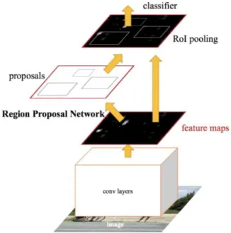
The third method is faster R-CNN. It is proposed by Shaoqing Ren et al. on the basis of fast R-CNN. Instead of using selective searching algorithm to predict the region proposals, it uses a region proposal network to do so. The method can significantly save time for detection because selective searching algorithm is a time-consuming process.

(14)

Figure 2.3: Faster R-CNN method overview (Ren et al. 2016)

The last method is You Only Look Once (YOLO) algorithm proposed by Joseph Redmon et al. All of the above methods use regions to localize the objects; the convolutional neural network does not look at the whole image, but the parts that have a high probability of containing the objects. YOLO algorithm, however, uses a single convolutional neural network to predict the bounding box together with the class probabilities. In the algorithm, the input image is split into an S×S grid, and within every grid, m bounding boxes are generated. The network outputs the class probability and offset values for each of the bounding boxes, and the bounding boxes with the probability larger than the threshold will represent the objects detected. Yolo neural network is very simple and fast. It processes images in real time at 45 frames per second.

(15)

2.2 Vehicle Tracking Method

Vehicle tracking aims to estimate the motion parameters, calculate the corresponding trajectories, and predict the upcoming position of vehicles. In vehicle detection, the bounding box of the vehicles and the locations of the bounding box are already obtained. The bounding box can be the representation of the vehicles in the tracking process. There are two types of methods for vision-based vehicle tracking: methods with prior knowledge and methods without prior knowledge (Liu et al. 2013).

Methods with prior knowledge include template match method and mean shift method. Template match method looks for a specific template from vehicle image and uses certain correlation to match and recognize vehicle in both steady state and dynamic state images (Fieguth et al. 1997). It is simple and precise but takes a long implementing time. Mean shift method uses a non-parameter density gradient estimator based on a general kernel function to analyze the image. If the kernel function meets the requirement, the estimation would be asymptotic unbiased, continuous, and consistent with the true value (Comaniciu et al. 2003).

Methods without prior knowledge include Kalman filter method, extended Kalman filter method, unscented Kalman filter method, and particle filter method.

Kalman filter method is suitable for linear state-space models. It uses a series of measurements over time, including noise and uncertainty to estimate the upcoming state. The dynamic model is used to predict the upcoming state, and the upcoming state is estimated using the prediction as well as the new measurement. The information imposed by the dynamic model significantly improves the tracking performance. (Gustaffson 2018)

Extended Kalman method and unscented Kalman filter method are suitable for nonlinear state-space models. Extended Kalman filter method linearize the nonlinear models at a certain point, so the Jacobian matrix around the point needs to be calculated. Unscented Kalman filter collects a set of deterministic samples and propagates them on the nonlinear function to calculate the means and covariance. (Gustaffson 2018)

Particle filter is suitable for both linear and nonlinear state-space models. It uses a set of random samples with important weights to estimate the upcoming state. The important weights indicate the relevance of each sample. The dynamic model is used to propagate the samples; the measurement update evaluates the likelihood to assign an importance

(16)

weight to each sample; re-sampling is used to mitigate particle degeneracy. When the number of sampled particles is large enough, the samples can sufficiently describe the probability density distribution. (Gustaffson 2018)

2.3 Method Selection

For vehicle detection method, methods based on machine learning are being considered. Compared to the classifier-based method, YOLO method has the following advantages. First, it looks at the entire image at once so that the prediction can be notified through the global context of the image. Secondly, it predicts through a single network evaluation, so it is very fast and suitable for real-time detection. Thirdly, YOLO has universality and extensive suitability. When it is extended from natural images to other fields such as works of art, it is superior to other methods. Fourthly, YOLO detects an object in each grid cell. It enhances spatial diversity in forecasting. A good example is Ojala et al. apply YOLO algorithm to localize pedestrians in real-time with high accuracy. Therefore, YOLO algorithm is selected as the vehicle detection method.

For vehicle tracking methods, methods without prior knowledge are being considered. Generally, Kalman filter method is suitable for linear model; extended Kalman filter method is suitable for weakly nonlinear model; unscented Kalman filter is suitable for highly nonlinear model; particle filter method is for both linear and nonlinear model (Zhao et al. 2015). Unscented Kalman filter is not selected due to its computational complexity. Therefore, Kalman filter method, extended Kalman filter method and particle filter method will be adopted and compared in the following context. The flowchart of vision-based vehicle detection and tracking is shown in Figure 2.5.

(17)

Figure 2.5 Flowchart of vision-based vehicle detection and tracking

2.4 Existing Literature

Having decided the thesis approaches, some literature relating to the topics are introduced here. The first topic is about using YOLO-based algorithm to detect the traffic participants; another topic is about utilizing the filtering algorithm to track the vehicles.

2.4.1 Literature about Vehicle Detection

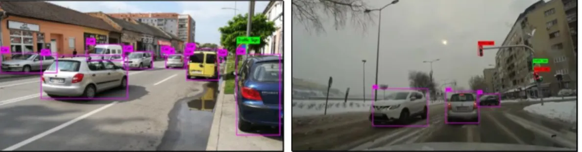
Aleksa Corovic et al. (2018) use YOLO algorithm to detect real-time traffic participants. They train the algorithm for five categories: car, truck, pedestrians, traffic signs, and traffic lights. The result shows that YOLO algorithm is suitable for real-time detection, and all of the objects close to the camera are successfully detected. They point out that the failure of detection occurs in two situations: the first is in high dense traffic area when one cell of the detection grid contains more than three objects; the other is when some objects are blocked by others. They also compare the detection results in different weathers and declare that the accuracy of the algorithm could be improved by training from a larger and more diverse dataset covering various weather and lighting conditions.

(18)

Figure 2.6: Detection visualization examples in sunny (left) and snowy (right) weathers (Aleksa Corovic et al. 2018)

Zhi Xu et al. (2018) propose a vehicle detection system under UAV based on optimal dense YOLO method. For vehicle detection under aerial view angle of UAV platform, the background information is complex and the vehicle target is small. To solve the problem, they combine YOLO algorithm with dense topology and optimal pooling. The result shows the model is significantly improved in extracting features of the small target. It also presents better accuracy and robustness, while maintaining the fast speed of YOLO algorithm.

Figure 2.7: YOLO v2 detection result (left) and optimal dense YOLO method detection result (right) (Zhi Xu et al. 2018)

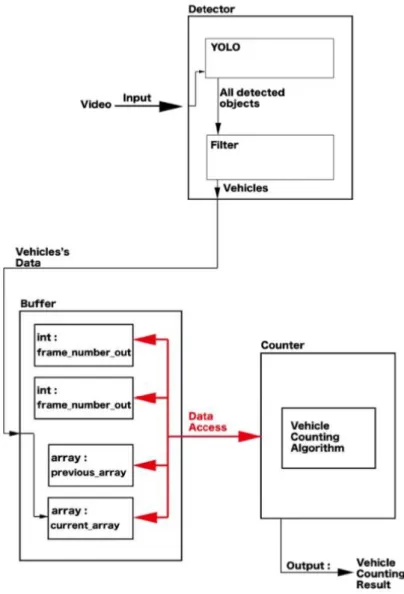
Jiaping Lin et al. (2018) develop a YOLO-based traffic counting system. The system consists of three modules, the Detector that generates the bounding boxes of the vehicles, the Buffer that stores the vehicle coordinates, and the Counter responsible for counting the vehicles. Video is input to the Detector where passing through YOLO and filter. Data access is built among frame number input and output, previous and current array in Buffer, and vehicle counting algorithm in Counter. They also add checkpoints to verify the validity of the detection. The correctness and overall efficiency of the system are evaluated by using video from different positions and angles. The results show that the system achieves high accuracy in the light-rich environment.

(19)

Figure 2.8: Architecture of traffic counting system (Jiaping Lin et al. 2018)

Jing Tao et al. (2017) build an object detection system for images in the traffic scene. They developed an optimized YOLO method called OYOLO by removing the last two fully connected layers and adding an average pool layer. The new network is faster than YOLO while exceeding other region-based methods in accuracy such as R-CNN. Combing OYOLO and R–FCN algorithm, the detection becomes more accurate. They also add a pre-processing procedure for night images by removing highlights, enhancing contrast and increasing brightness. The results show the new object detection system in the traffic scene is fast, accurate, and robust.

(20)

Figure 2.9: Speed (left) and accuracy (right) of OYOLO method compared with other object detection methods (Jing Tao et al. 2017)

2.4.2 Literature about Vehicle Tracking

Amir Salarpour et al. (2011) develop an algorithm to realize multiple vehicle tracking using Kalman filter and feature. First, they use background subtraction approach to detect the vehicles. Then they utilize both region-based and feature-based algorithms to track the vehicle. For region-based tracking, they use Kalman filter to predict the region of the vehicle in the next frame. And for feature-based tracking, they use color and size features to correct the results of the prediction. The result reflects that the method can solve the problem such as appearance, disappearance, and occlusion, thus it can distinguish and track all the vehicles individually in clutter scene with high accuracy.

Figure 2.10: Multi-vehicle tracking in clutter scene (Amir Salarpour et al. 2011)

Daniel Ponsa et al. (2005) present a multiple vehicle 3D tracking method using unscented Kalman filter. They use a monochrome camera platform installed on vehicles facing the road ahead with an inclination angle and determine the host coordinate system based on the camera position. Then a three-dimensional dynamic model of the system is established, in which the platform and the tracked vehicle are represented by state vectors. Combining the different observed values, a set of two-dimensional areas for vehicle

(21)

searching is obtained. The state vector is reevaluated by unscented Kalman filter from measurements obtained in every frame. After testing in long sequences, the results proved to be reliable even under poor acquisition conditions.

(22)

3. Mathematical Framework of the Vehicle

In order to detect and track the vehicle, the mathematical framework of the vehicle needs to be established. The concept of sensor fusion is employed here, which composed of sensor, variable of interest, models and estimation algorithm (Gustafsson 2018). Sensor, variable of interest, and models are established in this chapter, and estimation algorithm is discussed later in chapter 4.2.

Figure 3.1: Basic concept of sensor fusion

The variable of interest is the time-varying state of a dynamic system that can be measured directly or indirectly. The state can be measured directly is the pixel location of the vehicle at each time step t_n, consisting of x-coordinate and y-coordinate. According to different indirect states, two models are established, Wiener velocity model and quasi-constant turn model. The former one is a linear model, while the latter one is a nonlinear model.

The derivation of equations takes reference of the work by Fredrik Gustafsson (2018).

3.1 Wiener Velocity Model

The movement of the vehicle can be determined by its acceleration, as shown in Figure 3.2.

Figure 3.2: The movement of the vehicle determined by its acceleration

𝐚𝐲(t)

(23)

Assume the acceleration along x-axis and y-axis is random, it can be denoted as:

𝒗̇(t) = 𝐚(t) = [𝜔1(𝑡)

𝜔₂(𝑡)] (1)

where 𝜔₁(𝑡) and 𝜔₂(𝑡) are stochastic quantity with variance 𝛿_𝜔2_.

Set the variable of interest 𝒙(𝑡) as:

𝒙(𝑡) = [𝑝𝑥(𝑡) 𝑝𝑦_{(𝑡) 𝑣}𝑥_{(𝑡) 𝑣}𝑦_(𝑡)]𝑇 ₍₂₎

The state-space model is:

[ 𝑝̇𝑥_(𝑡) 𝑝̇𝑦_(𝑡) 𝑣̇𝑥_(𝑡) 𝑣̇𝑦(𝑡)] = [ 0 0 1 0 0 0 0 1 0 0 0 0 0 0 0 0 ] [ 𝑝𝑥_(𝑡) 𝑝𝑦_(𝑡) 𝑣𝑥_(𝑡) 𝑣𝑦(𝑡)] + [ 0 0 0 0 1 0 0 1 ] [𝜔1(𝑡) 𝜔₂(𝑡)] (3)

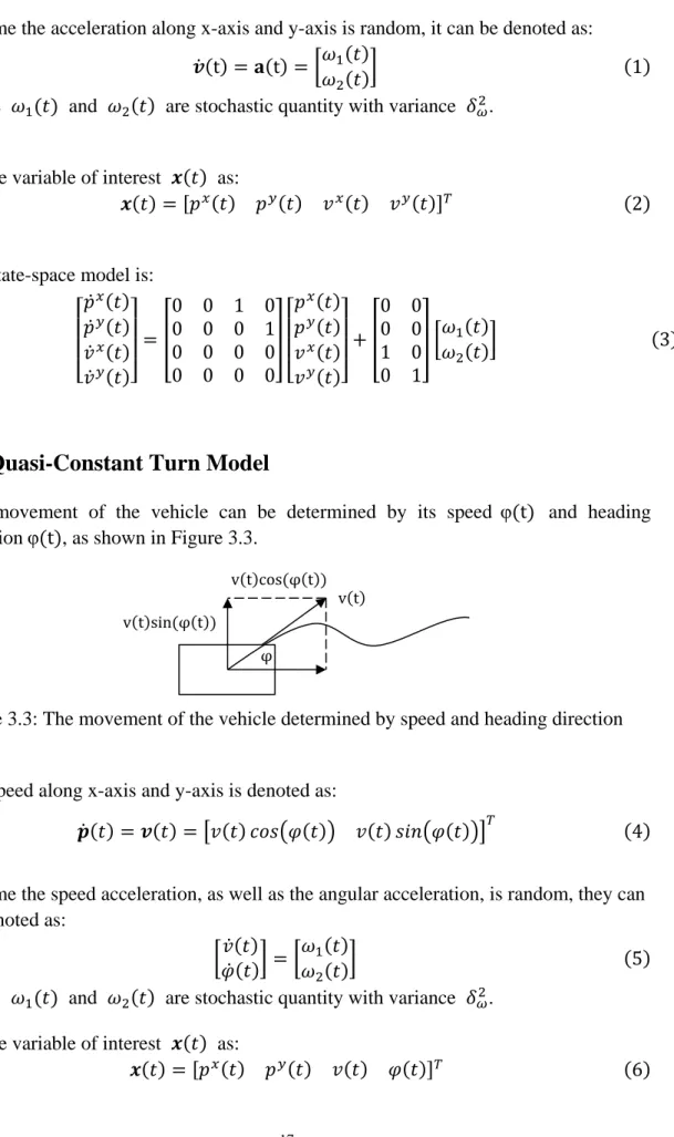
3.2 Quasi-Constant Turn Model

The movement of the vehicle can be determined by its speed φ(t) and heading directionφ(t), as shown in Figure 3.3.

Figure 3.3: The movement of the vehicle determined by speed and heading direction

The speed along x-axis and y-axis is denoted as:

𝒑̇(𝑡) = 𝒗(𝑡) = [𝑣(𝑡) 𝑐𝑜𝑠(𝜑(𝑡)) 𝑣(𝑡) 𝑠𝑖𝑛(𝜑(𝑡))]𝑇 (4)

Assume the speed acceleration, as well as the angular acceleration, is random, they can be denoted as:

[𝑣̇(𝑡) 𝜑̇(𝑡)] = [

𝜔₁(𝑡)

𝜔₂(𝑡)] (5)

where 𝜔₁(𝑡) and 𝜔₂(𝑡) are stochastic quantity with variance 𝛿_𝜔2.

Set the variable of interest 𝒙(𝑡) as:

𝒙(𝑡) = [𝑝𝑥(𝑡) 𝑝𝑦_{(𝑡) 𝑣(𝑡) 𝜑(𝑡)]}𝑇 ₍₆₎

v(t) v(t)sin(φ(t))

v(t)cos(φ(t))

(24)

The state-space model is: [ 𝑝̇𝑥(𝑡) 𝑝̇𝑦(𝑡) 𝑣̇(𝑡) 𝜑̇(𝑡) ] = [ 𝑣(𝑡) 𝑐𝑜𝑠(𝜑(𝑡)) 𝑣(𝑡) 𝑠𝑖𝑛(𝜑(𝑡)) 0 0 ] + [ 0 0 0 0 1 0 0 1 ] [𝜔1(𝑡) 𝜔₂(𝑡)] (7)

3.3 Sensor Model

A sensor is a device that provides a measurement of a variable of interest. The sensor, in this case, is the road camera that is used to record the traffic scene.

The sensor measurement is affected by measurement noise, and it represents the coordinates along x-axis and y-axis. So, for both of Wiener velocity model and quasi-constant turn model, the sensor model is:

𝒚_𝑛 = 𝑮_𝑛𝒙_𝑛 + 𝒓_𝑛 (8)

where

𝑮_𝑛 = [1 0 0 0

0 1 0 0] (9)

𝒓𝑛is the measurement noise, which is a multivariate random variable with probability

density function, which can be denoted as:

𝒓_𝑛~𝑝(𝒓_𝑛) (10)

Assume it is a zero-mean, independent random variable with covariance 𝑹_𝑛, it can be represented as:

𝐸{𝒓_𝑛} = 0, 𝐶𝑜𝑣{𝒓_𝑛} = 𝑹_𝑛 (11)

3.4 Discretization of

the State-Space Model

The measurement of the vehicle location is sampled at each time step 𝑡𝑛, so the

continuous state-space models need to be discretized. Discretization of the models is equivalent to solving the stochastic differential equation between 𝑡_𝑛−1 and 𝑡_𝑛.

3.4.1 Discretization of Wiener Velocity Model

Wiener Velocity Model is a stochastic linear dynamic model:

(25)

𝒙̇(𝑡) = 𝑨𝒙(𝑡) + 𝑩_𝜔𝛚(t) (12)

Multiply the integrating factor e−𝐀t we get:

𝑒−𝑨𝑡_{𝒙̇(𝑡) = 𝑒}−𝑨𝑡_{𝑨𝒙(𝑡) + e}−𝐀t_𝑩 𝜔𝝎(𝑡) (13) Rearranging it we get: 𝑒−𝑨𝑡𝒙̇(𝑡) − 𝑒−𝑨𝑡𝑨𝒙(𝑡) = e−𝐀t𝑩𝜔𝝎(𝑡) (14) Substituting d dt𝑒 −𝑨𝑡_{𝒙(𝑡) = 𝑒}−𝑨𝑡_{𝒙̇(𝑡) − 𝑒}−𝑨𝑡_{𝑨𝒙(𝑡)}_{we get:} d dt𝑒 −𝑨𝑡_{𝒙(𝑡) = e}−𝐀t_𝑩 𝜔𝝎(𝑡) (15)

Integrate it with respect to t we get:

∫ 𝑑 𝑑𝑡𝑒 −𝑨𝑡_{𝒙(𝑡)𝑑𝑡} 𝑡_𝑛 𝑡𝑛−1 = ∫ 𝑒−𝑨𝑡𝑩𝜔𝝎(𝑡) 𝑡_𝑛 𝑡𝑛−1 𝑑𝑡 (16) 𝑒−𝑨𝑡𝒙(𝑡_𝑛) − 𝑒−𝑨𝑡_𝑛−1_𝒙(𝑡 𝑛−1) = ∫ 𝑒−𝑨𝑡𝑩𝜔𝝎(𝑡) 𝑡𝑛 𝑡𝑛−1 𝑑𝑡 (17)

The solution is:

𝒙(𝑡_𝑛) = 𝑒𝑨(𝑡_𝑛−𝑡_𝑛−1)_𝒙(𝑡

𝑛−1) + ∫ 𝑒𝑨(𝑡𝑛−𝑡)𝑩𝜔𝝎(𝑡) 𝑡𝑛

𝑡𝑛−1

𝑑𝑡 (18)

It can be written as:

𝒙_𝑛 = 𝑭_𝑛𝒙_𝑛−1+ 𝒒_𝑛 (19) where 𝑭_𝑛 ≡ 𝑒𝑨(𝑡𝑛−𝑡𝑛−1) _{= 𝑰 + 𝛥𝑡𝑨} (20) 𝒒_𝑛 ≡ ∫ 𝑒𝑨(𝑡𝑛−𝑡)_𝑩 𝜔 𝑡𝑛 𝑡_𝑛−1 𝝎(𝑡)𝑑𝑡 (21)

𝝎(𝑡) is a white noise process and 𝑅_𝜔𝜔(𝜏) = 𝜎_𝑤2_𝛿(𝜏)

The process noise 𝒒𝑛 satisfies:

(26)

𝑸_𝑛 = 𝐶𝑜𝑣{𝒒_𝑛} = ∫ 𝑒𝑨(𝑡𝑛−𝜏)_𝑩 𝜔 𝑡𝑛 𝑡_𝑛−1 𝜎_𝑤2_𝑩 𝜔 𝑇_𝑒𝑨𝑇(𝑡_𝑛−𝜏)_𝑑𝜏 ₍₂₃₎

Substitute in the matrices we get:

𝑭𝑛 = [ 1 0 𝛥𝑡 0 0 1 0 𝛥𝑡 0 0 1 0 0 0 0 1 ] (24) 𝑸_𝑛 = 𝜎_𝜔2 [ (𝛥𝑡)3 3 0 (𝛥𝑡)2 2 0 0 (𝛥𝑡) 3 3 0 (𝛥𝑡)2 2 (𝛥𝑡)2 2 0 𝛥𝑡 0 0 (𝛥𝑡) 2 2 0 𝛥𝑡 ] (25)

Therefore, the discrete time state-space model is:

{ [ 𝑝_𝑛𝑥 𝑝_𝑛𝑦 𝑣𝑛𝑥 𝑣_𝑛𝑦] = [ 1 0 𝛥𝑡 0 0 1 0 𝛥𝑡 0 0 1 0 0 0 0 1 ] [ 𝑝_𝑛−1𝑥 𝑝_𝑛−1𝑦 𝑣_𝑛−1𝑥 𝑣_𝑛−1𝑦 ] + 𝒒_𝑛 𝒚_𝑛 = 𝑮_𝑛𝒙_𝑛+ 𝒓_𝑛 (26) with 𝐸{𝒒_𝑛} = 0, 𝐶𝑜𝑣{𝒒_𝑛} = 𝑸_𝑛 (27) 𝐸{𝒓𝑛} = 0, 𝐶𝑜𝑣{𝒓𝑛} = 𝑹𝑛 (28)

3.4.2 Discretization of Quasi-Constant Turn Model

Quasi-Constant Turn Model is a stochastic nonlinear dynamic model:

𝒙̇(𝑡) = 𝑓(𝒙(𝑡)) + 𝑩_𝜔(𝒙(𝑡))𝛚(t) (29)

First, the model is linearized around 𝒙𝑛−1 using first order Taylor series approximation:

(27)

𝒙̇(𝑡) ≈ 𝑓(𝒙_𝑛−1) + 𝑨𝑥(𝒙(𝑡) − 𝒙𝑛−1) + 𝑩𝜔(𝒙(𝑡))𝛚(t) (31)

where 𝑨_𝑥 is the Jacobian matrix of 𝑓(𝒙(𝑡)) at 𝒙_𝑛−1.

Substitute in the matrices we get:

𝑨𝑥 = [ 0 0 cos(𝜑_𝑛−1) −𝑣𝑛−1sin(𝜑𝑛−1) 0 0 sin(𝜑_𝑛−1) 𝑣_𝑛−1cos(𝜑_𝑛−1) 0 0 0 0 0 0 0 0 ] (32)

Then the model is discretized in the same way:

𝒙_𝑛 = 𝒙_𝑛−1+ ∫ 𝑒𝑨(𝑡𝑛−𝑡)_𝑑𝑡 𝑡𝑛 𝑡𝑛−1 𝑓(𝒙_𝑛−1) + ∫ 𝑒𝑨(𝑡𝑛−𝑡)_𝑩 𝜔 𝑡𝑛 𝑡𝑛−1 (𝒙(𝑡))𝝎(𝑡)𝑑𝑡 (33) 𝑭_𝑥≡ 𝑒𝑨𝑥(𝑡𝑛−𝑡𝑛−1) _{= 𝑰 + 𝛥𝑡𝑨} 𝑥 = [ 1 0 𝛥 tcos(𝜑_𝑛−1) −𝛥𝑡𝑣𝑛−1sin(𝜑𝑛−1) 0 1 𝛥 tsin(𝜑_𝑛−1) 𝛥𝑡𝑣_𝑛−1cos(𝜑_𝑛−1) 0 0 1 0 0 0 0 1 ] (34) 𝒒_𝑛 ≡ ∫ 𝑒𝑨(𝑡𝑛−𝑡)_𝑩 𝜔 𝑡𝑛 𝑡_𝑛−1 (𝒙(𝑡))𝝎(𝑡)𝑑𝑡 (35) with 𝒒_𝑛~𝑁(0, 𝑸_𝑛) (36) 𝑸_𝑛 = 𝐶𝑜𝑣{𝒒_𝑛} = ∫ 𝑒𝑨(𝑡𝑛−𝜏)_𝑩 𝜔 𝑡𝑛 𝑡_𝑛−1 𝜎_𝑤2_𝑩 𝜔 𝑇_𝑒𝑨𝑇(𝑡_𝑛−𝜏)_𝑑𝜏 ₍₃₇₎

However, it is still hard to determine 𝑸_𝑛. So, Euler-Maruyama method is used here.

The stochastic nonlinear dynamic model is:

𝒙̇(𝑡) = 𝑓(𝒙(𝑡)) + 𝑩𝜔(𝒙(𝑡))𝛚(t) (38)

The integral representation is:

𝒙_𝑛 = 𝒙_𝑛−1+ ∫ 𝑓(𝒙(𝑡)) 𝑡𝑛 𝑡_𝑛−1 𝑑𝑡 + ∫ 𝑩_𝜔(𝒙(𝑡))𝛚(t) 𝑡𝑛 𝑡_𝑛−1 𝑑𝑡 (39)

(28)

By Euler-Maruyama discretization:

𝒙𝑛 = 𝒙𝑛−1+ 𝛥𝑡𝑓(𝒙𝑛−1) + 𝒒𝑛 (40)

The process noise is:

𝒒𝑛 ≡ ∫ 𝑩𝜔(𝒙(𝑡))𝛚(t) 𝑡_𝑛 𝑡𝑛−1 𝑑𝑡 (41) with 𝒒𝑛~𝑁(0, 𝑸𝑛) (42) 𝑸𝑛 = 𝐶𝑜𝑣{𝒒𝑛} = ∫ 𝑩𝜔 𝑡_𝑛 𝑡𝑛−1 (𝒙(𝑡))𝜎𝑤2𝑩𝜔𝑇(𝒙(𝑡))𝑑𝜏 (43)

Using rectangle approximation, we get:

𝑸𝑛 = 𝐶𝑜𝑣{𝒒𝑛} ≈ 𝛥𝑡𝑩𝜔(𝒙𝑛−1)𝜎𝑤2𝑩𝜔(𝒙𝑛−1)𝑇 (44)

The discrete time state-space model is:

{ [ 𝑝_𝑛𝑥 𝑝_𝑛𝑦 𝑣_𝑛 𝜑_𝑛 ] = [ 𝑝_𝑛−1𝑥 𝑝_𝑛−1𝑦 𝑣𝑛−1 𝜑𝑛−1] + [ 𝛥𝑡𝑣_𝑛−1cos(𝜑_𝑛−1) 𝛥𝑡𝑣_𝑛−1sin(𝜑_𝑛−1) 0 0 ] + 𝒒_𝑛 𝒚_𝑛 = 𝑮_𝑛𝒙_𝑛+ 𝒓_𝑛 (45) with 𝐸{𝒒𝑛} = 0, 𝐶𝑜𝑣{𝒒𝑛} = 𝑸𝑛 (46) 𝐸{𝒓_𝑛} = 0, 𝐶𝑜𝑣{𝒓_𝑛} = 𝑹_𝑛 (47)

(29)

4. Simulation of Vehicle Detection and Tracking

4.1 Simulation of Vehicle Detection

The aim of vehicle detection is to extract the vehicle from the video and locate it within the image. The traffic video is a simulation of the traffic scene at a crossroad recorded by a driving simulator called BeamNG.drive. In the 5-second video, the detection target is a single car, and it is making a turn from the top right side to the bottom left side. There are no pedestrians, bikes, or other vehicles passing through the region of detection.

4.1.1 Generation of Image Sequence

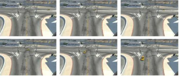
In order to conduct vehicle detection, the video is converted into an image sequence. Set the frame rate to be 10fps, 52 frames are generated. Figure 4.1 shows a subset of the frames.

Figure 4.1: Frame 1, frame 10, frame 20, frame 30, frame 40 and frame 50 in the image sequence of the traffic scene

4.1.2 Adoption of YOLO Algorithm

YOLO is a network inspired by GoogleNet. It has twenty-four convolutional layers working as feature extractors and two dense layers to make predictions. The framework is called Darknet, which is also created by Redmon et al. Darknet uses mostly 3 × 3 filters to extract features, 1 × 1 filters to reduce output channels, and a global average pooling to make predictions (Hui 2018). The flowchart of YOLO network with Darknet is shown in Figure 4.2.

(30)

Figure 4.2: Flowchart of YOLO network with Darknet (Hui 2018)

The algorithm used in the simulation is YOLO v3 from open source. In YOLO v3, a new 53-layer Darknet-53 is used as the feature extractor, instead of the 19-layer Darknet-19 used in YOLO v2. Darknet-53 mainly consists of 3 × 3 and 1× 1 filters with skip connections similar to the residual network in ResNet. Darknet-53 has less billion floating point operations than ResNet-152, but it is two times faster with the same classification accuracy. (Redmon et al. 2018)

Figure 4.3: Darknet-19 in YOLO v2 (left, Redmon et al. 2017) and Darknet-53 in YOLO v3 (right, Redmon et al. 2018)

The simulation uses the pre-trained weights for object detection. The model is trained on COCO dataset, which includes 123287 images and 886284 instances. The results are divided into 80 categories shown in Figure 4.4.

(31)

Figure 4.4: 80 catagories in COCO dataset (http://cocodataset.org)

Detect objects with YOLO v3 algorithm using the pre-trained weights in each frame by running the following command:

darknet.exe detect cfg/yolov3.cfg yolov3.weights

The default input image size of YOLO v3 is 416 × 416 pixels, which affects accuracy and computational load. Real-time detection can be achieved with higher input sizes, for example 608×608 pixels. The default detection threshold is 0.25, which affects the output number of class categories. The threshold can be adjusted according to the needs. Default values are used here for vehicle detection.

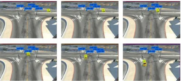
Enter the file path of every frame, and Darknet prints out the object categories, the confidence, and the time it takes to find them. Figure 4.5 shows the detection results corresponding to the frames in Figure 4.1.

Figure 4.5: Object detection in frame 1, frame 10, frame 20, frame 30, frame 40 and frame 50 using YOLO algorithm

(32)

The vehicle can be detected in all the images, except that in the 18th image, it is blocked by the traffic lights.

4.1.3 Statistic Analysis

Select the bounding box of the vehicle in each frame and extract the left, top, right, bottom coordinates of the bounding box. The pixel location of the vehicle center can be obtained in each frame, as shown in Table 4.1. In the table, left, top, right, bottom are the offset values of the bounding box, 𝑐_𝑥is the x-coordinate of the bounding box center, and 𝑐𝑦is the y-coordinate of the bounding box center.

Table 4.1: Characteristic coordinates of the vehicle in each frame

Left Top Right Bottom 𝒄_𝒙 𝒄_𝒚

1 1398 259 1503 296 1450 277 2 1375 259 1482 295 1428 277 3 1357 260 1460 295 1408 277 4 1335 261 1435 295 1385 278 5 1313 262 1410 296 1361 279 6 1286 261 1392 296 1339 278 7 1267 260 1367 295 1317 277 8 1243 260 1344 296 1293 278 9 1218 259 1318 296 1268 277 10 1197 259 1298 296 1247 277 11 1175 259 1271 296 1223 277 12 1150 256 1247 297 1198 276 13 1126 258 1225 295 1175 276 14 1110 257 1204 295 1157 276 15 1105 254 1182 294 1143 274 16 1063 256 1161 296 1112 276 17 1041 259 1144 294 1092 276 18 \ \ \ \ \ \ 19 1011 261 1083 289 1047 275 20 981 258 1078 298 1029 278 21 963 259 1053 300 1008 279 22 945 256 1043 302 994 279 23 923 265 1026 305 974 285 24 903 265 1000 307 951 286 25 885 266 983 310 934 288 26 869 269 968 313 918 291

(33)

27 853 270 948 318 900 294 28 834 275 929 321 881 298 29 820 279 915 329 867 304 30 804 282 905 331 854 306 31 795 286 891 338 843 312 32 780 292 874 342 827 317 33 766 299 860 351 813 325 34 749 304 845 358 797 331 35 745 310 824 364 784 337 36 724 316 818 375 771 345 37 709 322 807 382 758 352 38 705 327 792 392 748 359 39 692 340 779 405 735 372 40 682 348 765 414 723 381 41 677 358 754 427 715 392 42 664 371 743 445 703 408 43 653 380 732 460 692 420 44 647 395 723 472 685 433 45 631 406 716 497 673 451 46 629 411 713 513 671 462 47 625 438 703 537 664 487 48 603 450 704 565 653 507 49 598 479 699 586 648 532 50 589 500 690 623 639 561 51 585 530 688 660 636 595 52 575 555 682 703 628 629

4.2 Simulation of Vehicle Tracking

Vehicle tracking aims to estimate the motion parameters, calculate the corresponding trajectories, and predict the upcoming position of vehicles in the image. Since the measurement points of the sensor are obtained in the “𝑐_𝑥” and “𝑐_𝑦” columns in Table 4.1,

they can be put into the mathematical model of the vehicle to realize vehicle tracking. Three methods are compared here, Kalman filter method, extended Kalman filter method, and particle filter method.

(34)

4.2.1 Kalman Filter Method

Kalman filter method iterates two steps for all measurement points in sequence. The first step is the prediction, which aims to predict the current state using the dynamic model. The second step is measurement update, which aims to estimate the current state using the prediction and the new measurement.

The objective is to estimate the current state 𝒙_𝑛 given the new measurement 𝒚_𝑛, taking the prediction into account.

𝒙

̂_n|ndenotes the estimated value at 𝑡_𝑛, given the measurements 𝒚_1:𝑛 = {𝑦₁, 𝑦₂, … , 𝑦_𝑛},

𝐏n|n denotes the covariance at 𝑡𝑛.

The initial condition is 𝒙̂_0|0= 𝒎₀, 𝑷_0|0= 𝑷₀. For n=1,2, …

The prediction is:

𝒙

̂_n|n−1= 𝑭_𝑛𝒙̂_n−1|n−1 (48) 𝐏_n|n−1 = 𝑭_𝑛𝐏_n−1|n−1𝑭_𝑛𝑇_{+ 𝑸}

𝑛 (49)

Using regularized squares as the estimation algorithm to estimate𝒙_𝑛:

J_RELS(𝒙_𝑛) = (𝒚_𝑛 − 𝑮_𝑛𝒙_𝑛)𝑇_𝑹 𝑛 −1_(𝒚 𝑛− 𝑮𝑛𝒙𝑛) + (𝒙_𝑛 − 𝒙̂_n|n−1)T𝐏_n|n−1(𝒙_𝑛− x̂_n|n−1) (50) and solve 𝒙 ̂_𝑛|𝑛 =𝑎𝑟𝑔𝑚𝑖𝑛 𝒙𝑛 𝐽𝑅𝐸𝐿𝑆(𝒙𝑛) (51)

The measurement update is:

𝐊_n = 𝐏_n|n−1𝑮_𝑛𝑇_(𝑮 𝑛𝐏n|n−1𝑮𝑛𝑇+ 𝑹𝑛) −1 (51) 𝒙 ̂_𝑛|𝑛 = 𝒙̂_n|n−1+ 𝐊_n(𝒚_𝑛− 𝑮_𝑛𝒙̂_n|n−1) (52) 𝐏_n|n = 𝐏_n|n−1− 𝐊_n(𝑮_𝑛𝐏_n|n−1𝑮_𝑛𝑇 _{+ 𝑹} 𝑛)𝐊nT (53)

(35)

4.2.2 Extended Kalman Filter Method

Extended Kalman Filter first linearizes the dynamic model, then it also iterates the same two steps for all measurement points in sequence. The objective is also to estimate the current state 𝒙_𝑛 given the new measurement 𝒚_𝑛, taking the prediction into account.

The initial condition is 𝒙̂_0|0= 𝒎0, 𝑷0|0= 𝑷0.

First, the dynamic model is linearized around 𝒙̂_n−1|n−1:

𝒙_𝑛 = 𝑓(𝒙_𝑛−1) + 𝒒_𝑛 ≈ 𝑓(𝒙̂_{𝑛−1|𝑛−1}) + 𝑭_𝑥(𝒙_𝑛−1− 𝒙̂_{𝑛−1|𝑛−1}) + 𝒒_𝑛 (54)

For n=1,2, … The prediction is:

𝒙

̂_{𝑛|𝑛−1}= 𝐸{𝒙_𝑛|𝒚_1:𝑛−1}

≈ 𝐸{𝑓(𝒙̂_{𝑛−1|𝑛−1}) + 𝑭_𝑥(𝒙_𝑛−1− 𝒙̂_{𝑛−1|𝑛−1}) + 𝒒_𝑛|𝒚_1:𝑛−1} = 𝑓(𝒙̂_{𝑛−1|𝑛−1}) (55)

𝑷_{𝑛|𝑛−1}= 𝐸 {(𝒙_𝑛− 𝒙̂_{𝑛|𝑛−1})(𝒙_𝑛− 𝒙̂_{𝑛|𝑛−1})𝑇|𝒚_1:𝑛−1}

= 𝑭𝑥𝑷𝑛−1|𝑛−1𝑭𝑥𝑇+ 𝑸𝑛 (56)

Using regularized squares as the estimation algorithm to estimate𝒙_𝑛:

J_RELS(𝒙_𝑛) = (𝒚_𝑛− 𝑮_𝑛𝒙_𝑛)𝑇_𝑹 𝑛 −1_(𝒚 𝑛 − 𝑮𝑛𝒙𝑛) + (𝒙_𝑛 − 𝒙̂_n|n−1)T𝐏_n|n−1(𝒙_𝑛− x̂_n|n−1) (57) and solve 𝒙 ̂_𝑛|𝑛= 𝑎𝑟𝑔𝑚𝑖𝑛 𝒙_𝑛 𝐽𝑅𝐸𝐿𝑆(𝒙𝑛) (58)

The measurement update is:

𝐊n = 𝐏n|n−1𝑮𝑛𝑇(𝑮𝑛𝐏n|n−1𝑮𝑛𝑇+ 𝑹𝑛) −1 (59) 𝒙 ̂_𝑛|𝑛 = 𝒙̂_n|n−1+ 𝐊_n(𝒚_𝑛 − 𝑮_𝑛𝒙̂_n|n−1) (60) 𝐏_n|n = 𝐏_n|n−1− 𝐊_n(𝑮_𝑛𝐏_n|n−1𝑮_𝑛𝑇_{+ 𝑹} 𝑛)𝐊nT (61)

(36)

4.2.3 Particle Filter Method

The particle filter method also iterates the same two steps, prediction and measurement update. However, there are J sets of states sampled instead of one. And the particles in each set are evaluated respectively.

The initial condition is 𝒙₀𝑗~𝑁(𝒎₀, 𝑷₀ ). For n=1,2, …

In prediction, the simulated states 𝒙_𝑛−1𝑗 (𝑗 = 1,2, … 𝐽) are given. And 𝒙_𝑛𝑗 (𝑗 = 1,2, … 𝐽) is obtained by simulating from t_𝑛−1 to t_𝑛.

For 𝑗 = 1,2, … 𝐽, Sample 𝒒_𝑛𝑗 ~𝑁(0, 𝑸𝑛) and propagate particles:

𝒙_𝑛𝑗 = 𝑭_𝑛𝒙_𝑛−1𝑗 + 𝒒_𝑛𝑗 (𝑗 = 1,2, … 𝐽) (62)

In measurement update, 𝒙_𝑛𝑗 is evaluated by how well it explains 𝒚𝑛 and assigned to a

weight.

𝜔̃_𝑛𝑗 = 𝑝(𝒚_𝑛|𝒙_𝑛𝑗) = 𝑁(𝒚_𝑛; 𝑮_𝑛𝒙_𝑛𝑗, 𝑹_𝑛)(𝑗 = 1,2, … 𝐽) (63)

Normalize the particle weights:

𝜔_𝑛𝑗 = 𝜔̃𝑛

𝑗

∑𝐽_𝑖=1𝜔̃_𝑛𝑗(𝑗 = 1,2, … 𝐽) (64)

And calculate 𝒙̂_𝑛|𝑛, 𝐏_n|n.

To prevent particle degeneracy after a few samples, the particles are resampled by removing samples with low weights and replicate samples with high weights so that:

Pr{𝒙̃_𝑛𝑖 _{= 𝒙} 𝑛 𝑗

} = 𝜔_𝑛𝑗 (65)

4.3 Simulation Result

Using Kalman filter method, extended Kalman filter method and particle filter method respectively. For Kalman filter method and particle filter method, Wiener velocity model is adopted; and for extended Kalman filter method, quasi-constant turn model is adopted. The measurement noise covariance is set as 1 × 𝑒𝑦𝑒(2). The variance of stochastic vector is set as 500. For particle filter method, the number of particles J is set to be 1000.

(37)

The code of applying particle filter for tracking simulation is shown in appendix 4, and the code of applying Kalman filter and extended Kalman filter are later shown in chapter 5.2. The simulation results of vehicle detection and tracking of the three methods are shown in Figure 4.6-4.8.

Figure 4.6: Detection and tracking result of Kalman filter method

(38)

Figure 4.8: Detection and tracking result of Particle filter method

The performance of the two methods can be assessed in the following two ways. The first way is to measure the precision of the data. This can be realized by calculating the root mean square error (RMSE):

e_RMSE= √1 N∑(x̂n|n− xn) T (x̂_n|n− x_n) N n=1 (66)

where x̂_n|n is the estimated value and x_nis the measurement value.

Since the detection result of YOLO algorithm can be bouncing around the target due to the noise factors, the second way is to measure the fluctuation degree of the data. In order to do this, the points on the fitting trajectory are collected with the same x-coordinates of the estimated value, and the fluctuation error is calculated by:

e_fluc= √1 N∑(x̂n|n− xn′) T (x̂_n|n− x_n′) N n=1 (67)

(39)

The RMSE and fluctuation error of Kalman filter method (KF), extended Kalman filter method (EKF) and particle filter method (PF) are shown in Table 4.2, and translated into Figure 4.9 for analysis.

Table 4.2 RMSE and fluctuation error of different methods

KF EKF PF

𝐞_{𝐑𝐌𝐒𝐄}(pixels) 2.53 2.59 3.29

𝐞_{𝐟𝐥𝐮𝐜} (pixels) 1.61 3.01 2.58

Figure 4.9: Chart of RMSE error and fluctuation error of different methods

It can be seen that the errors of the three methods are of the same order of magnitude. For RMSE error, Kalman filter method and extended Kalman filter method are more accurate than particle filter method. For fluctuation error, Kalman filter method surpasses the other two methods, which means it is less likely to be affected by the noise factors. Particle filter method, however, conducts numerical calculation on each step instead of the estimation algorithm, so it has lower computational complexity. Particle filter method also overcomes the constraint of a single Gaussian distribution of Kalman filter and extended Kalman filter methods (Liu et al. 2013). However, in the simulation, only one set of data is collected by the road camera, which could not sufficiently describe the probability density distribution. Therefore, Kalman filter method and extended Kalman filter method are more feasible than particle filter method, and they are selected as the vehicle tracking method in the practical experiment.

0 2 4

RMSE Fluctuation Error

Pix

els

RMSE and Fluctuation Error of Different

Methods

Kalman filter method Extended Kalman filter method Particle filter method

(40)

5. Practical Experiment

The simulation result is quite promising. However, in real life, the case is much more complicated. It is a challenge to deal with the occlusion problem of multiple targets in a scene and the data correlation among them (Liu et al. 2013). Besides, the traffic scenes in real life can be very complicated, many factors such as shadow, reflection and weather conditions could affect the result of vehicle detection and tracking. These require higher robustness and adaptive ability.

5.1 Experiment of Vehicle Detection

The video is recorded by the test camera installed towards a crossroad at Aalto University. Cars, trucks, pedestrians, bikes pass through the region of detection from time to time, and there is a construction site which blocks part of the view of the objects behind. A video clip of 40 seconds is intercepted and set as the experiment target.

5.1.1 Real-Time Vehicle Detection

Real-time detection is achieved by combing Darknet and OpenCV. Run the following command:

darknet.exe detector demo cfg/coco.data cfg/yolov3.cfg yolov3.weights <traffic video>

YOLO displays the detection categories, class probability, current FPS on the command window, together with the image with bounding boxes.

The detection frame rate depends on the computational capability of the computer. The computer specifications are listed in Table 5.1.

Table 5.1: Computer specifications of real-time detection

System Specification

CPU Intel Core i7-7700 3.6Ghz

RAM 32Gb DDR4 2666Mhz

GPU Nvidia Geforce GTX 1080

(41)

As a result, 1227 frames are captured during the process, showing object categories such as cars, persons, trucks, and traffic lights. The average frame rate of the 1227 frames is 42.5 fps, which means real-time detection is achieved.

Though the detection frame rate is time-varying, it is fluctuating around the average within a narrow range. To simplify the calculation, the sampling rate is set as 42.5 fps. During the video clip, two trucks and seven cars are detected at the traffic scene.

5.1.2 Statistic Analysis

By adding the following line to the function “draw_detections” in the file “image.c”:

Printf (“%f %f %f %f \n”, b.x, b.y, b.w, b.h);

The characteristic coordinates of different objects are displayed in the command window in each frame. For example, in the first frame (shown in Figure 5.5), the coordinates are shown in Table 5.2. In the table, c_x is the x-coordinate of the bounding box center,

c_y is the y-coordinate of the bounding box center, w is width of the bounding box, and h is the height of the bounding box.

(42)

Table 5.2: Characteristic coordinates of frame 1 Category Confidence 𝒄_𝒙 𝒄_𝒚 w h truck: 77% 0.512026 0.395793 0.086306 0.156872 car, truck: 65%, 57% 0.328256 0.625595 0.060951 0.143655 car: 85% 0.204036 0.261504 0.041046 0.032712 car: 93% 0.257539 0.279898 0.044714 0.027226 car: 44% 0.991706 0.316585 0.011802 0.040050 person: 75% 0.207041 0.419650 0.013232 0.053896 car: 88% 0.821291 0.292883 0.061517 0.051907 person: 94% 0.120525 0.702477 0.026776 0.093496 car: 99% 0.853219 0.325227 0.075767 0.050247

To get the coordinates of the vehicles, the first step is to keep the data of the vehicles including cars and trucks; and delete the data of other categories such as persons, bikes, and traffic lights. Then the static objects are removed, for example, the parking cars on the right side. Then the “cx” and “cy” columns collected in each frame composed of the measurement data.

5.2 Experiment of Vehicle Tracking

Knowing the coordinates of all the vehicles in 1227 frames, the next step is to find out the trajectory of the vehicles by figuring out their correlations. The biggest challenge, as mentioned above, is to distinguish which coordinates belong to which vehicle, since the occlusion of multiple targets occurs at all times. This requires an identification algorithm, which assumes that the vehicle is the same one when the range between two measurement points is within the threshold.

5.2.1 Identification Algorithm

The idea of the algorithm is to put the initial points of different vehicles into a temporary matrix. Comparing the points with the new point in each frame, if the range of the two points is smaller than the threshold, the new point will be added below the old point in

(43)

the temporary matrix and removed from the frame matrix. Every matching string is stored as the trajectory of a car. The string is considered ended when no match could be founded in the new frame. Otherwise, the remaining points that could not find a match from previous strings in the frame will be added to the temporary matrix, made starts of new strings, and continue comparing. To get rid of accidental errors. The strings that are too short are eliminated. The flowchart of the identification algorithm is shown in Figure 5.6, and the code is shown in Appendix 1.

Figure 5.6: Flowchart of the identification algorithm

By running the code, point sequences are obtained in each cell of the result. In order to get the measurement points of each vehicle, Minimum length of the point sequences, as

(44)

well as the threshold of point matching, needs to be tuned. However, in some cases the point sequences are discontinuous since the detection is not always ideal; to solve the problem, the point sequences need to be stitched. The final result of the measurement points of each vehicle in saved in an Excel document.

5.2.2 Applying Filtering Algorithm

The next step is applying filters to the point sequence of each vehicle to realize tracking. Kalman Filter and extended Kalman filter are applied to calculate the trajectory and predict the upcoming position. The flowchart of applying Kalman filter and extended Kalman filter for tracking experiment is shown in Figure 5.7, and the codes are shown in Appendix 2-3. The measurement noise covariance is set as 0.1 × 𝑒𝑦𝑒(2). The variance of stochastic vector is set as 104.

Figure 5.7: Flowchart of applying Kalman filter and extended Kalman filter for tracking experiment

(45)

5.3 Experiment Result

5.3.1 Detection and Tracking Result

The detection and tracking results of part of the vehicles are shown in Figure 5.8-5.12.

Kalman filter method

Extended Kalman filter method

Figure 5.8: detection and tracking result of Car 2

Pixel s Pixel s Pixels Pixels

(46)

Figure 5.9: Detection and tracking result of Car 3

(47)

(48)

(49)

Figure 5.12: Detection and tracking result of Truck 2

The RMSE and fluctuation error of each vehicle are listed in Table 5.3, and translated into Figure 5.13 and Figure 5.14 for analysis.

(50)

Table 5.3: RMSE and fluctuation error of each vehicle ( |𝑹_𝒏| = 𝟎. 𝟏, 𝝈𝒘𝟐 = 𝟏𝟎𝟒 )

Vehicle KF Method EKF Method

RMSE (pixels) Fluct. Error (pixels) RMSE (pixels) Fluct. Error (pixels) Car 1 2.79 3.03 3.82 3.72 Car 2 2.67 3.41 3.08 3.14 Car 3 0.92 3.06 1.84 2.78 Car 4 1.03 / 1.98 / Car 5 1.22 / 1.89 / Car 6 3.53 1.89 3.74 1.71 Car 7 1.55 3.26 2.33 2.97 Truck 1 1.83 2.58 3.50 3.20 Truck 2 3.12 / 4.16 / Average 2.07 2.87 2.92 2.92

Figure 5.13: Chart of RMSE of different vehicles

0 1 2 3 4

Car 1 Car 2 Car 3 Car 4 Car 5 Car 6 Car 7 Truck 1 Truck 2

Pix

els

RMSE of Different Vehicles

(51)

Figure 5.14: Chart of fluctuation error of different vehicles

For both of the methods, the RMSE are within 4.5 pixels, and the fluctuation errors are within 4 pixels. So, the overall results achieve high accuracy and stableness. Kalman methods surpasses extended Kalman method in precision, and the two methods have similar performance in stableness.

There are a few points to note here. First, the interference factors could result in the loss of the measurement points where the machine vision is not detecting the vehicle for a while. For example, the measurement points of Truck 2 are not regular due to the occlusion by construction fence and shadows in the experiment.

This is the scenario where YOLO are not able to provide any measurements of the vehicle for a short period of time. Therefore, we would have to estimate the trajectory of the vehicle during that time. Assuming the 50th to 70th measurement points are lost, the tracking result for Car 2 during that period of time are shown in Figure 5.15.

0 1 2 3 4

Car 1 Car 2 Car 3 Car 6 Car 7 Truck 1

Pix

els

Fluctuation Error of Different Vehicles

(52)

Figure 5.15: Tracking result for Car 2 when 50th to 70th measurement points are lost

For both Kalman filter method and extended Kalman filter method, during the period of lost measurement, the estimation points will follow the same gradient of the last measurement until it receives the new measurement. As a consequence, the fluctuation error of this period jumps to zero, but the RSME significantly increases because the trajectory becomes a line and deviates from the measurement points.

To estimate how long a vehicle can be undetected before the error becomes substantial, we set different time steps of the lost measuremt and compare the maximum error (shown in Figure 5.15) during the period of lost measurement.

(53)

Table 5.4: Maximum error during the period of lost measurement for Car 2 with different lost time steps ( |𝑹_𝒏| = 𝟎. 𝟏, 𝝈𝒘𝟐 = 𝟏𝟎𝟒 )

Lost time steps KF Method EKF Method

Max error (pixels) Max error (pixels)

50th_{- 55}th _3.63 _5.09

50th_{- 60}th _13.96 _14.79

50th_{- 70}th _24.32 _27.57

50th_{- 80}th _30.49 _41.08

50th - 90th 51.48 73.41

From the table, it can be seen when the lost measurement is around 30 time steps, the RMSE of that period exceeds 30 pixels, which is assumed to be a substantial error. The footage was recorded at 30 FPS, so it can be estimated that when the loss of measurement data achieves 1 second, the positioning error caused by the lack of measurement data could not be neglected. This prediction method is naturally very prone to errors when the vehicle is taking a turn at the intersection, so the fragment that we assume to be lost here is not at the intersection. More sophisticated prediction is required for those scenarios.

Second, polynomial fitting is used for the trajectory fitting in the experiment. In statistics, polynomial fitting is a form of regression analysis in which the relationship between the independent variable x and the dependent variable y is modelled as an nth degree polynomial in x. In the experiment, x and y denote the x-coordinate and y-coordinate of the vehicle estimated position, so that we can plot the fitting trajectory of the vehicles. We use 10 degrees of polynomial fitting here.

However, polynomial fitting does not work effectively in some complex curve. For example, polynomial fitting is not feasible for Car 4, Car 5, and Truck 2, so the trajectories for these vehicles are plotted by simply connecting the discontinuous estimation points. Since the points collected from fitting trajectory are used as the standards to calculate the fluctuation errors, the fluctuation errors of these vehicles cannot be calculated.

Third, the precision of the estimation depends on the precision of the measurement data, because they are regarded as the standard values to evaluate RMSE. However, if

Vision-based vehicle detection and tracking in intelligent transportation system

Wencan Mao