An Effective Data-Driven Method for 3-D Building Roof Reconstruction and Robust Change Detection

Article

An Effective Data-Driven Method for 3-D Building

Roof Reconstruction and Robust Change Detection

1 _{School of Information and Communication Technology, Griffith University, Nathan, QLD 4111, Australia;}

[email protected] (S.A.N.G.); [email protected] (F.U.S.)

2 _{Faculty of Information Technology, Monash University, Clayton, VIC 3800, Australia}

* Correspondence: [email protected]; Tel.: +61-7-373-55032 † Authors contributed equally to this work.

Received: 13 June 2018; Accepted: 19 September 2018; Published: 21 September 2018 Abstract:Three-dimensional (3-D) reconstruction of building roofs can be an essential prerequisite for 3-D building change detection, which is important for detection of informal buildings or extensions and for update of 3-D map database. However, automatic 3-D roof reconstruction from the remote sensing data is still in its development stage for a number of reasons. For instance, there are difficulties in determining the neighbourhood relationships among the planes on a complex building roof, locating the step edges from point cloud data often requires additional information or may impose constraints, and missing roof planes attract human interaction and often produces high reconstruction errors. This research introduces a new 3-D roof reconstruction technique that constructs an adjacency matrix to define the topological relationships among the roof planes. It identifies any missing planes through an analysis using the 3-D plane intersection lines between adjacent planes. Then, it generates new planes to fill gaps of missing planes. Finally, it obtains complete building models through insertion of approximate wall planes and building floor. The reported research in this paper then uses the generated building models to detect 3-D changes in buildings. Plane connections between neighbouring planes are first defined to establish relationships between neighbouring planes. Then, each building in the reference and test model sets is represented using a graph data structure. Finally, the height intensity images, and if required the graph representations, of the reference and test models are directly compared to find and categorise 3-D changes into five groups:new,unchanged, demolished,modifiedandpartially-modifiedplanes. Experimental results on two Australian datasets show high object- and pixel-based accuracy in terms of completeness, correctness, and quality for both 3-D roof reconstruction and change detection techniques. The proposed change detection technique is robust to various changes including addition of a new veranda to or removal of an existing veranda from a building and increase of the height of a building.

Keywords:building; modelling; reconstruction; change detection; LiDAR; point cloud; 3-D

1. Introduction

The fundamental task of building reconstruction is the transformation of low-level building primitives (e.g., lines and planes) to a high-level model description. In 3-D change detection, it is inspected whether there are changes in buildings over a period in terms of new, modified, and/or demolished buildings and/or building-parts. The reconstruction step can be considered as an essential prerequisite for 3-D change detection, particularly for detection of informal buildings or extensions and for update of 3-D map database. In a 3-D map database, there are buildings along with other important man-made objects such as roads and electric power lines. A direct comparison of 3-D building models generated from a recent dataset to the models in the (old) map database will not

only identify the changes in buildings but also help an effective and efficient update of the database. In practice, there will be only a small number of buildings being changed in an area for a given period of time, unless this is a newly built-up area or an area hit by a calamity (e.g., bushfire or earthquake). Therefore, automatic modelling and change detection steps will be helpful in indicating the potential changed areas of buildings in a user interface, where a human operator can quickly accept and/or reject the indications and update the database accordingly [1]. Moreover, the state and local government officials can check if the indicative changes were previously authorised or not. Thus, they can send inspectors to the unauthorised (informal) areas only, instead of all areas, saving both money and time.

Many scientists have developed building reconstruction and change detection techniques utilising image information only, others have utilised LiDAR (Light Detection And Ranging) point cloud, and some have attempted to integrate LiDAR and aerial images for several Geographic Information System (GIS) applications, including city mapping, map database updating, disaster estimation, and city infrastructure planning. However, among spatial data researchers and mapping professionals, LiDAR data have gained popularity because of fast pulsation, precision, and accuracy in capturing 3-D geo-referenced spatial information about buildings, roads, vegetation, and other objects expediently at a high point density. These characteristics make these data feasible to examine natural and built environments across a wide range of scales for automatic reconstruction and change detection in buildings and their distinct features. Recent improvements in the automation of building reconstruction and change detection methods are reducing the labour and time consumption in these applications.

The 3-D reconstruction of building models and change detection include several non-trivial processes, such as segmentation, classification, structuring, hypothesis generation, and geometric modelling. A seamless integration of these in a conventional way would be not only unrealistic but also labourious. This paper, therefore, presents a workflow that uses building roof planes for 3-D model generation and subsequently uses these models for change detection. To achieve our goals and address the particular challenges, this research presents two techniques aiming at 3-D reconstruction of building roof models and building change detection separately. The proposed techniques are entirely data-driven using LiDAR point cloud data only. The first technique, 3-D building roof modelling, reconstructs buildings represented at lower levels with coarse boundaries (3-D roof planes) to higher levels (3-D building models). The second technique, building change detection, subsequently uses the constructed 3-D building models and LiDAR data for identification of changes in buildings.

In Section2, the related works are discussed. Section3provides the detail on challenges for 3-D building modelling and change detection methods, along with the contributions of this paper. The proposed 3-D building modelling and 3-D change detection methods are presented in Sections4 and5, respectively. In Section6, the dataset, parameter settings, experimental setup, and results are discussed. Finally, conclusions are presented in Section7.

2. Related Works

In recent years, studies on building extraction, reconstruction and change detection have made significant advances and a wide range of methods have been proposed on façade segmentation and opening area detection [2], building extraction [3–5], change detection and map database update [1,6–8], roof plane extraction [9] and 3-D reconstruction [10]. A number of techniques [11,12] have also been proposed for evaluation of these methods. In addition, since different methods were evaluated using different datasets and evaluation techniques, there have been several attempts to benchmark them on common platforms [13,14].

In 3-D building roof reconstruction and change detection most early methods were manual, with the involvement of a trained human operator who performed accurate measurements. However, human intervention is not only expensive but also reduces the speed of execution in achieving high productivity and in processing large datasets. Recently developed reconstruction and change detection methods [1,15] aim to reduce these limitations in a semiautomatic manner.

2.1. 3-D Building Roof Modelling

The 3-D building reconstruction methods can broadly be classified into three categories on the basis of their processing strategies: model-driven, data-driven, and hybrid approaches [16–18]. A model-driven method uses a set of predefined building models (shape) and fits into the input data for the extraction purposes, in contrast to a data-driven method that uses the input data and extracts one or more features (e.g., lines and planes) for the detection and reconstruction of buildings. A hybrid method, on the other hand, exhibits the characteristics of both model- and data-driven approaches.

Among the model-driven methods, Oude Elberink and Vosselman [19] proposed a graph matching approach to handle both complete and incomplete laser data. While a complete matching of data with a target model allows an automated 3-D reconstruction of a building roof, an incomplete match leads to a manual interaction for a correct model. To reduce human interaction, Xiong et al. [20] proposed a graph-based error correction for roof topology. A graph edit dictionary that stores representative erroneous subgraphs was used to automatically identify and correct errors.

Kim and Shan [10] proposed a novel data-driven roof plane segmentation and building reconstruction technique using airborne LiDAR data. Although this technique shows good results, it suffers from over-segmentation and neglects the effect of vegetation in the segmentation process. Jung et al. [21] presented a reconstruction technique to develop 3-D rooftop models at city-scale from LiDAR data. Although the experimental results showed a good performance for large buildings, some small roof planes were not detected, and were therefore not reconstructed. Moreover, this method suffers from under-segmentation issues since many roof planes were merged into their adjacent clusters. Wu et al. [22] offered a graph-based technique to reconstruct urban building models from airborne LiDAR data. Building models were reconstructed by gluing all individual parts of the building models obtained from bipartite graph matching into a complete model. Although this technique provides detailed models, it fails to capture the sides of buildings and produces high geometric distortion resulting in low completeness and high modelling errors.

Rottensteiner et al. [14] reported comparative research results for urban object detection and 3-D building reconstruction using the ISPRS (International Society for Photogrammetry and Remote Sensing) benchmark datasets. They selected fourteen different building reconstruction methods and evaluated their performances on the basis of different quality metrics.

2.2. 3-D Building Change Detection

Based on the input data sources, the building change detection methods can be categorised into three groups: image only, LiDAR only or integration of LiDAR and image-based methods. The image-based methods are mainly for 2-D change detection and are mostly unable to differentiate between partially-modified buildings and planes. For example, both Gu et al. [8] and Leichtle et al. [7] divided the image region into changed and unchanged buildings only and were unable to find out the changes in individual roof planes.

Raw LiDAR data or LiDAR-derived Digital Surface Model (DSM) is also used as the only source of information to detect the 3-D building changes [6,23]. Tran et al. [6] proposed a method where, in addition to the ground and tree, they classified buildings into new, demolished and unchanged types. Teo and Shih [23] extracted changed building regions by applying the height threshold and morphological filter to nDSM (normalised DSM) of two different days. However, this method missed many small planes because of inadequate selection of window size of the filter. In addition, this method was unable to detect partially-modified building planes.

There are also methods that use a segmentation technique for building change detection from both LiDAR and images [1,24]. For instance, Awrangjeb [1] generated a building mask by extracting the building boundaries from non-ground LiDAR data. Later, the building boundaries were refined manually using visual analysis of the aerial image. This method could detect all possible changes in a building such as new, demolished, unchanged, modified, and partially-modified buildings.

In addition, there are also methods that detect the changes in a building using 3-D building models. These methods compare the height information of individual buildings and detect the height changes in the buildings for change detection. A 3-D building model can be generated from LiDAR data by using thresholding method [25] or from stereo-images by using a least square matching process [26,27]. For example, Chen et al. [25] used LiDAR-based building models at two different dates to detect building changes. The non-building portion of the models was removed by using a height threshold and NDVI (Normalized Difference Vegetation Index) analysis. However, small changes in buildings and occluded buildings were also removed from the models and were not detected. Therefore, this method had up to 96% of pixel-based accuracy. Stal et al. [26] and Qin [27] methods compare the stereo-images- and LiDAR-based building models to detect building changes. In the method of Stal et al. [26], a morphological filter and NDVI analysis were applied to remove the unwanted regions, while Qin [27] used three more filters, such as shadow index, noise filter, and irregular structure filter. However, the methods that use 3-D building models need several pre-defined parameters for accurate detection of building changes. In addition, modified and partially-modified building planes were not detected by these methods.

3. Challenges and Contributions

The existing 3-D building modelling techniques differ significantly, based on the primitive shapes used and the input data sources [28]. They often impose constraints on the minimum footprint size and positional accuracy values for reconstruction of specific models at a certain level of detail [29]. Although many of the existing approaches have demonstrated promising results in building reconstruction, there are still a number of issues to be improved. For instance, building roofs are mostly disconnected after segmentation process, causing difficulty in determining the neighbourhood relationships among the roof planes. Furthermore, locating step edges from LiDAR data only is also hard and often requires additional information or constraints. In addition, the approximation of roof patches, which are generally missed because of the low density of the LiDAR data, requires the operator to make assumptions and often produces high reconstruction errors.

To resolve the above issues, this research introduces a data-driven 3-D reconstruction technique that constructs buildings represented at lower levels with coarse boundaries (3-D roof planes) to the higher levels (3-D building models). The proposed reconstruction technique receives building roof planes (extracted from LiDAR point could data by any roof plane extraction method such as Awrangjeb and Fraser [9] and Mongus et al. [4]) as inputs and offers the following contributions:

• Insertion of missing planes: A missing plane can be a small plane from where the number of reflected laser points is limited, possibly due to a low point density. It can also be due to a height jump between planes. A slanted plane is grown if there is an existence of unsegmented LiDAR points between any two planes. Otherwise, a vertical plane is inserted between the planes.

• Reconstruction of complete building models: When there are missing planes, the topological relationship among the roof planes is incorrect. Thus, an adjacency matrix that defines the topological relationships among the input roof planes of a building is first constructed. Then, the matrix is updated (i.e., the topological relationship is corrected) based on the inserted missing planes. Finally, the building model is generated using the correct topological relationship and the revised intersection lines among the inserted missing planes and the input roof planes.

Generally, the building change detection step is applied after the building detection or 3-D building modelling stage to update a map database [1]. The update to the map database is largely dependent on visual interpretation, estimation of numerous parameters, and human interaction. Consequently, it is a time-consuming procedure to analyse the changes. In addition, most of the existing methods mainly focus on detecting the 2-D changes in a building and, thus, are unable to distinguish the specific height change in individual planes. Moreover, majority of the existing 3-D change detection methods, which are based on height difference in the DSM, classify the detected changes into three

groups: new, unchanged and demolished planes [23,25,30]. Consequently, these methods are unable to distinguish the partially-modified planes from the unchanged and new planes, and modified planes from the new planes. Therefore, the contribution of the proposed building change detection technique can be summarised as follows:

• Change detection: Automatic detection of 3-D (2-D space and height) changes in buildings and their planes into five groups:new,unchanged,demolished,modified, andpartially-modifiedplanes. Unlike the existing methods, the proposed method is capable of detecting changes on a per-plane basis. A newly proposed graphical representation of 3-D building models helps in identification ofmodifiedandpartially-modifiedplanes.

Since in reality only a small number of buildings are changed in an area, the proposed change detection technique first uses height difference values between the reference and test models to identify new, completely demolished and unchanged buildings. The planes of these buildings are denoted as new,demolishedandunchanged, respectively. Then, only the modified building regions are compared using a graph-based representation of the reference and test models to obtain other changes such as modifiedandpartially-modifiedplanes.

4. Proposed 3-D Building Modelling Technique

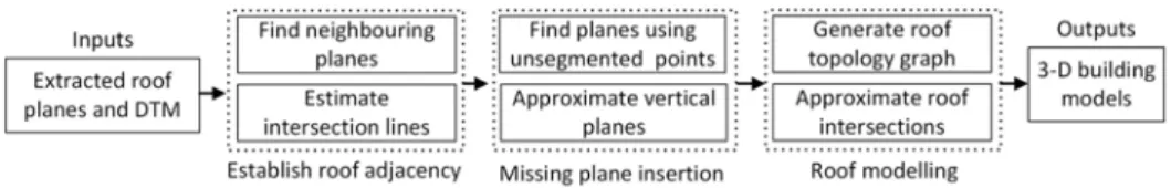
Figure1shows the workflow of the proposed 3-D building modelling technique. Awrangjeb and Fraser’s [9] technique is used for the extraction of building roof planes using LiDAR data and the corresponding Digital Terrain Model (DTM) as the input. The used technique offers high detection performance but has low accuracy in extracting small roof planes and tiny structures since it uses only the LiDAR data. This section presents the different steps in Figure1in detail for generation of 3-D building models.

4.1. Adjacency of Roof Planes and Their Intersection Lines

The primary elements for the generation of building models are the roof planes which are input to the proposed technique. A neighbourhood relation matrix is established among the roof planes to determine the topological relations among these 3-D roof primitives, which is originally an adjacency matrix and stores the records of the neighbours of each roof plane.

LetSp={P1,P2, ...,Pn}be a set ofninput roof planes and an adjacency matrixMof the same size is instantiated, i.e.,Mn×n. The roof planes that remain within the Euclidean distancedistpof a source planePiare considered its neighbours and the corresponding rows and columns ofMare updated accordingly with the roof plane’s ID. The value ofdistpis chosen as twice the maximum distance (dmax) of a point to its nearest point in the input LiDAR point cloud [9]. To speed up the generation ofM, the planes within an appropriate rectangular region (e.g., a bit larger than the bounding box) around the source planePiare first determined, rather than computing the distances of a planePito the rest of the input roof planes. Next, for the planes which lie withindistpof the boundary points ofPi, their particular records against theith row and column ofMare updated. The procedure continues and all the input roof planes are processed iteratively to establish the interrelations among them.

Then, to find the intersection line between two adjacent planesP1andP2, their plane equations

are used to assess whether these planes mutually intersect in 3-D space. If they do, a point called the intersection pointIpntand a direction vector ˆnin 3-D space are obtained. The two end points of the intersection line are not known fromIpnt and ˆnalone. Subsequently, 2-D straight lines are first approximated using the roof boundary points which face each other. The MATLAB built-in function polyfitis used for the approximation of line segments. Following the concepts of 3-D coordinate geometry and using the approximated 2-D lines,Ipnt, and ˆntogether, the 3-D intersection lines between the adjacent roof planes are estimated.

Figure 1.The workflow of the proposed 3-D building modelling technique.

The position ofIpntfrom the two corresponding plane boundaries is considered, entirely according to the resolution of the input LiDAR data, to bedistp = 2dmax. The plane insertion procedure first assesses the nearest distances ofIpntfrom two intersecting plane boundaries. If any of the two nearest distances exceeds 2dmax, it will potentially indicate either of the two general possibilities: (1) a missing LiDAR-based plane; or (2) a missing vertical plane, between these adjacent roof planes. Both o possible scenarios are described using diagrams in the following sections.

4.2. Detection and Insertion of Missing Roof Planes

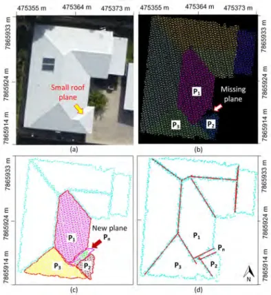
The proposed modelling technique now iteratively takes a plane and its neighbours to approximate their intersection lines. However, if the position of Ipnt is away (more than 2dmax) from the two intersecting plane boundaries, the plane insertion process attempts to search for any unsegmented LiDAR points between the participating roof planes. If such points are found (at least 4) , the process infers the presence of a plane between these roof planes. Figure2a,b shows an example building and a small missing plane among already extracted planesP1,P2, andP3.

The process invokes the region-growing segmentation technique in Awrangjeb [9] to extract a planar regionPnusing the unsegmented LiDAR points (see the green points in Figure2c). In addition to the available points, the segmentation process uses points of the neighbouring planes (P1,P2, and

P3) for the extraction of a new planePnassuming these points might have been added wrongly to the neighbouring planes becausePnwas missed earlier. Therefore, each iteration of the region-growing technique computes a plane-fitting error between new and neighbouring planes. If the new plane results in a height error smaller than those of the neighbouring planes’ errors, the LiDAR points of the neighbouring planes are removed from their respective regions and added toPn.

The segmentation process continues growing the region until it finds no points complying with the above height error criterion. After the segmentation process stops, the proposed technique estimates the boundary of the new plane and updates the boundary information of the neighbouring planes, as shown in Figure2c. The process also updates the neighbourhood matrixMwith the information on the new plane and new neighbouring relations. Subsequently, the intersection lines between the identified plane and the participating planes are estimated using their boundary points, as explained in Section4.1. These intersection lines are also recorded against their adjacent roof planes. Figure2d shows all the roof planes of the sample building and the intersection lines between them.

Figure 2.Insertion of a missing plane: (a) test building image for demonstration; (b) input roof planes for corresponding building and the location of a missing plane; (c) new roof plane using unsegmented LiDAR points (green) and points from neighbours; and (d) 3-D intersection lines between roof planes. 4.3. Insertion of Vertical Roof Planes

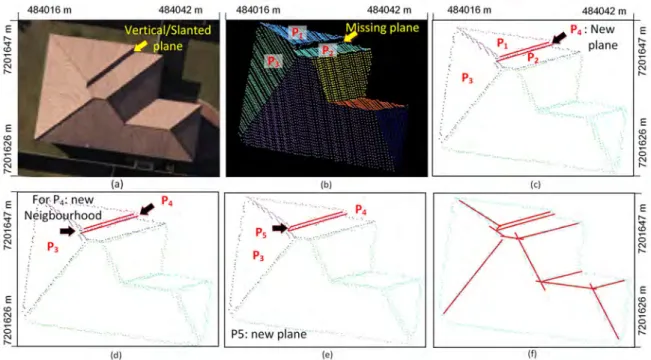
Figure3a shows a building, where a small slanted plane is located between two adjacent roof planes labelledP1andP2. This plane was not detected by the involved segmentation technique due

to the unavailability or absence of enough LiDAR points, as shown in Figure3b. Therefore, a new planeP4betweenP1andP2is inserted as follows. The neighbouring boundary points ofP1andP2are

first used to form a vertical planeP4. Then, the intersection lines ofP4withP1andP2, respectively,

are determined. Figure3c shows P4 and its intersection lines withP1 andP2 . The procedure not

only keeps track of new planes, but also maintains the correct neighbourhood information in M. Therefore, even after the insertion ofP4, it is found through the neighbourhood selection method

(described in Section4.1) thatP4has a new neighbouring plane, i.e., P3, as can be seen visually in

Figure3b,d. There is a dire need to determine the intersection betweenP3andP4to precisely establish

the topological relationships among the building roofs and reconstruct a model with a good level of detail.

As shown in Figure3,P4 is actually a thin slanted (nearly vertical) plane. However, due to

shortage of points on this plane, it could not be inserted using LiDAR data following the procedure in Section4.2. Since a vertical plane is inserted instead, the intersection line betweenP3andP4cannot

be found as expected. To solve this, the plane insertion procedure is executed following the similar steps above and a new vertical planeP5is inserted betweenP3andP4using their boundary points.

The procedure further approximates the intersection lines between the participating roof planes, betweenP3andP5and betweenP5andP4, as shown in Figure3e. The procedure stops once all the

roof planes are processed. Figure3f shows all the building roof planes and their intersection lines in 3-D space for better visualisation.

Thereafter, the boundary of each building is extracted using the boundary tracing procedure in Ali et al. [31] and regularised using the technique proposed by Awrangjeb [32] to form an appropriate building footprint, which is a polygon consisting of 3-D corner points.

Figure 3.Insertion of a real vertical plane: (a) test building image for demonstration; (b) input roof planes for corresponding building and location of missing plane; (c) insertion of a new vertical planeP4;

(d) assessing adjacency between existing planeP3and new planeP4; (e) insertion of a new vertical plane

P5betweenP3andP4; and (f) 3-D view of building roof planes and intersection lines for construction

of interrelation between roof planes. 4.4. Rooftop Topology and Modelling

At this juncture, the information about the buildings, all their possible roof planes, intersection lines, and the adjacency relationship is available. For 3-D roof modelling, it is important to obtain 3-D ridge (intersection of ridge lines) and edge (intersection of ridge line and building boundary) points. However, as shown in Figure4a, there is a small gap between each end point of a ridge line and its corresponding (actual) ridge or edge points. To fill the gaps and establish connectivity among the adjacent roof planes, the adjacency matrixMis used along with the Roof Topology Graph (RTG) following the principles proposed by Verma et al. [33]. As shown in Figure4b, each roof plane is represented as a vertex in RTG and two adjacent planes are connected through an edge. These roof planes are labelled with their vertex numbers in Figure4a.

In the context of RTG, a basic cycle indicates a ridge point that belongs to several ridge lines [34]. For instance, the roof planesP1,P4, andP5form a basic cycle and the intersection of the corresponding

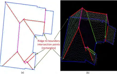
ridge lines determines a ridge intersection point. In addition, the corresponding vertices of the ridge lines participating in the intersection determination process are updated. These points can also be referred as ridge points, and will be used at the later stage to approximate the model shape. An RTG can also be represented as a composition of several basic cycles, as shown in Figure4c. The building rooftop shown in Figure4a has six basic cycles and so do the ridge intersection points. The least squares approach is applied to approximate the intersection among the ridge lines of the participating roof planes, as shown in Figure4d. Thereafter, 3-D edge points are found by intersecting ridge lines with the building boundary. Figure5a,b shows the edge points in two different perspective views. Note that, in a real scenario, two or more ridge lines intersect at the same point on the building boundary. However, the intersection of these ridge lines and the building boundary in the proposed modelling method may generate two or more individual points on the boundary. A 3-D single intersection point is not estimated for these points, since such an estimated 3-D single point may not be on the building boundary. Hence, individual edge points are considered.

1 3 2 4 5 6 7 8 (a) 3 2 1 4 6 5 8 7 1 3 2 4 5 6 7 8 (b) (d) (c) 3 1 4 3 2 1 4 6 5 4 6 7 8 6 7 5 1 4 Ridge gaps

Figure 4. Determination of ridge intersection points: (a) roof planes and ridge (intersection) lines; (b) Roof topology graph; (c) closed cycles; and (d) corresponding ridge intersection points.

Figure 5. Determination of edge intersection points: (a) edge points (ridge to building boundary intersection points); and (b) 3-D view of building showing edge points.

4.5. Complete 3-D Building Models

For roof modelling, each building is processed separately, and the procedure first finds the 3-D points around each plane boundary and constructs each roof segment. To do this, 3-D intersection lines, whose junction points (red ovals in Figure6) have been updated, are recalled. Then, the junction points (edge or ridge points) of 3-D intersection lines are re-ordered in succession around the plane using the information on the corresponding LiDAR-based building boundary points. This is shown in Figure6a, where the junction points are labelled asN1–N6to represent a roof segment. All the

roof planes of each building are processed iteratively and the corresponding roof model is generated that has regularised plane boundaries, as shown in Figure6b. Note that during the above modelling process (e.g., using least squares to approximate the intersection among the ridge lines), the planarity of the roof segment, say using the 3-D junction pointsN1–N6, may be slightly changed with respect to

the original plane equation generated from the segmented LiDAR points. However, the plane equation is not updated since it is estimated by a large number of LiDAR points on the plane.

For a complete 3-D building model, it is necessary to generate walls from the periphery of the roof model to its floor. In this regard, the edge points are used to generate the approximate building floor first. The ground height of each edge point is determined from the DTM so that the model seems to be a replica of its respective real building. All the consecutive ground points are connected to obtain the building floor. Finally, the building walls are determined by extruding the edge points to their corresponding floor points. Figure7presents the real building and its 3-D reconstructed model, where the walls are represented in a transparent grey colour.

(a) (b) N1 N2 N3 N4 N5 N6

Figure 6.Individual roof segments and building model: (a) a roof segment is shown with a sequence of ridge and edge points (N1toN6); and (b) roof model of the sample building.

Figure 7.Complete building model for the sample building: (a) aerial image; and (b) 3-D model. 5. Proposed 3-D Building Change Detection Method

Any building change detection method requires two sets of building models: a reference set and a test model set. The reference dataset is collected at an earlier date than that of the test dataset. For our investigation, however, datasets from two different dates were not available. Therefore, the 3-D models generated from the available dataset are considered to be in the reference model set and a model modification step is carried out to generate the test model set.

Figure8shows the flow diagram of the proposed building change detection method. The inputs to the proposed method are aerial images, LiDAR, DTM, and extracted 3-D building (reference) models. The proposed method has three major steps: (i) test model generation; (ii) creation of building data structure; and (iii) automatic change detection. The test model generation step is a manual step. If the test model set is generated from an available dataset captured at a later date than that of the reference dataset, then this step is not necessary.

Figure 8.The flow diagram of the proposed building change detection method.

To identify the changes, the reference and test models are represented in a graph-based data structure. Thereafter, they can be compared in the automatic change detection step. However, since the number of actual changes in buildings is small in practice, such a model-by-model comparison will be unnecessarily time consuming. Therefore, the height information of the test and reference models are first used to identify potential change locations. Then, the models are compared, if necessary, using the 3-D representations. Consequently, the planes from both models are classified into five groups: unchanged,new,modified,demolishedandpartially-modifiedplanes.

5.1. Test Model Generation

The building models generated by the proposed 3-D building modelling technique are considered as reference models. To obtain test models, the size and height changes are introduced to the reference models. Among the input data of the proposed change detection technique (see Figure8), while the aerial image contains sharp boundaries of objects including the buildings, the DTM and plane equation contain the bare earth and height information of buildings, respectively. Therefore, the DTM, plane equation, and aerial images are collectively used to produce changes in the reference data.

The changes in the reference data are performed by selecting points around a plane’s boundary in the aerial image and import X (Easting) and Y (Northing) coordinates of that location. This procedure is also shown in Figure9. Based on X and Y coordinates of a point, its Z (Height) value is approximated by using the respective plane equation. For the wall planes, Z value at a ground point of the wall plane is directly extracted from the DTM. The extracted information of planes is later used to modify the building model of the reference data. For example in Figure10, five different changes are made to the reference models: addition of height to two buildings, addition of a veranda to a building, removal of verandas from two buildings, addition of a new building, and relocation of all buildings in the scene. 5.2. 3-D Model Representation

Unlike the existing methods, the proposed 3-D change detection method not only obtains building changes on a per-plane basis, but also detectsmodifiedandpartially-modifiedplanes. A graph-based 3-D data structure, where individual planes and their relationships are represented, is proposed to detectmodifiedandpartially-modifiedplanes. The relationship between planes helps identification of different types of planes (e.g., roof and wall planes) and relative position of a plane with respect to its neighbouring planes. In addition, this ensures the detection of wall planes that are usually undetected by analysing only height change.

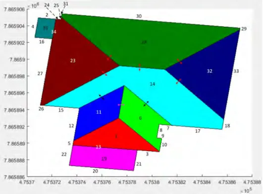
The 3-D building model consists of roof and wall planes. The relationship between the connected roof planes (indicated by the adjacency matrixM) can either be a parent-to-child, a parent-to-parent, or a child-to-child connection. The parent-to-parent and child-to-child are also called sibling connections. All connected roof planes are initially labelled as siblings. Then, the parent-to-child connection of two connected roof planes is labelled by verifying the two conditions: (1) the child and parent planes intersect each other; and (2) the child plane has a height value lower than the parent. Whereas the relationship between a roof plane and a wall plane is a parent-to-child connection, the relationship between two neighbouring wall planes is a child-to-child connection. Parents that intersect each other are in a parent-to-parent connection. For instance, in Figure11, the parent-to-child, parent-to-parent, and child-to-child connections are marked by black, red and magenta arrows, respectively, for the building shown in the orange coloured rectangle in Figure10a.

Figure 9. Extracting X and Y coordinates of a point of the cyan plane, where X and Y values are highlighted by a purple box.

Figure 10.Introduction of five different changes: (a) reference data; (b) addition of height to buildings; (c) addition of a veranda; (d) removal of verandas; (e) addition of a new building; and (f) relocation of building positions.

Thereafter, a 3-D building model is represented in a graphical structure, where each plane of a building is considered as a separate node. A node contains the complete information of a plane, e.g., plane ID, plane equation, 3-D plane points (i.e., polygon), plane type (i.e., roof or wall plane), and its connected plane information. Figure12shows an example to illustrate the data structure of a 3-D building model shown within the orange rectangle in Figure10a. The roof and wall planes are represented by blue and red nodes, respectively. As complete information of a node is not possible to mention in the data tree, the plane ID is shown at each node. The connections of nodes can either be sibling (parent-to-parent and child-to-child connections) or parent-to-child, which are highlighted by black and green coloured edges, respectively. The arrowhead of a green edge indicates the child in the parent-to-child relationship.

5.3. Automatic Building Change Detection

The proposed change detection method measures the change between the 3-D models of the reference and test scenes by comparing their structural information. The full structural comparison using the graphical representation, shown in Figure12, between the two corresponding building modelsBrandBt, from the reference and test model sets, respectively, is unnecessary for the following reasons. Firstly, the full comparison of all corresponding building pairs (Br,Bt) is computationally expensive. Secondly, in practice, there will be no or only a small number of existing buildings being changed in a given test scene. Therefore, the building structure of both models are first compared based on the height difference. Then, if necessary, only the related parts of the graph data structures are compared to obtain a more specific types and details of the involved changes. By using these two tests, the proposed method classifies the building planes into five groups:unchanged,demolished,new, modified, andpartially-modifiedplanes.

Figure 11. Relationship between the connected building planes; black, red, and magenta arrows represent the parent-to-child, parent-to-parent, and child-to-child connections, respectively. This building is the one within the orange rectangle in Figure10a and its wall plane numbers are shown outside the building boundary.

5.3.1. Height Test

For the height test, two intensity images are generated: one for the reference scene and the other for the test scene. Each intensity image has a resolution of 0.25 m and represents heights from individual roof planes with respect to the ground. Thus, a zero height represents no buildings. The input LiDAR points within the segmented planes from [9] are used to generate the height image. If the LiDAR points are not available, then the individual plane equations can be used to estimate heights on each pixel of the height image. In the height test, the height intensity image (say,Ir) of the reference scene is subtracted from that (say,It) of the test scene. Figure13c shows the absolute (pixel-to-pixel) height difference image (Id=It−Ir) forIrandItin Figure13a,b. InId, there can be the following cases for buildings in the scene (see Figure13). CaseA: For a completely new building, all height differences are positive inIdand there is only zero height value inIr. All planes within this new building are marked asnew. CaseB: Likewise, for a completely demolished building, all height differences are negative inIdand there is only zero height value inIt. All planes within this demolished building

are marked asdemolished. CaseC: If there are no or negligible height differences everywhere within a building region, then all of its planes are marked asunchanged. In reality, however, if the two models of an unchanged building are generated from two datasets obtained at different times, the final models can be slightly different. Therefore, a height tolerance threshold (0.5 m) is used. In addition, there may be non-overlapping thin parts (due to high height difference) along the building boundaries, this should not be more than 1 m in width for an unchanged building. Otherwise, the building is considered modified and CasesDandEbelow are considered.

If the above three cases (CasesA–C) fromIdare excluded, the remaining regions are all modified building regions in the scene. Figure13d shows the imageImcontaining only modified regions after exclusion of completely new, demolished and unchanged buildings fromIdin Figure13c. InIm, there can be the following cases for modified buildings in the scene. CaseD: A building is modified through removing one or more parts, e.g., a veranda is removed, which is shown within the orange rectangles in Figure10a,d. This case is observed by the same absolute height values within the corresponding modified region inImandIr, but zero height value in It. CaseE: A building is modified through extending one or more parts, e.g., a veranda is added or extended. This case is observed by the same absolute height values within the corresponding modified region inImandIt, but zero height value inIr(see Figure13d). CaseF: A building is modified in height direction, e.g., a one-storey building is modified to a two-storey building, or vice versa (see Figure13d). For these three cases, all the unchanged areas, if any, are identified and planes within these areas are markedunchanged(the same procedure is followed as in CaseCabove). Consequently, only the planes in each modified region in

Imare now subject to the plane test below exploiting the graphical representation in Figure12.

Figure 12. A graph (data structure) for a building model shown within the orange rectangle in Figure10a: roof planes are blue nodes; wall planes are red nodes; parent-to-child connections are in green edges (where an arrowhead indicates a child side); and sibling connections are in black edges.

Figure 13. Finding the 3-D plane changes between the reference and test models: Height intensity images for: (a) reference models; (b) test models; (c) absolute height difference image (test minus reference); and (d) modified building regions.

5.3.2. Plane Test

Let the two graphical representations ofBr andBtbeGr andGt, respectively. A removal of a building part (CaseD) is a result of a full and/or partially demolishment of one or more existing building planes. In this situation, the partially-demolished planes are present in bothGrandGt, but fully demolished planes are only present inGr. In contrast, an extension to an existing building (Case

E) consists of an addition of one or more completely new planes and/or an extension of one or more existing planes. In such a case, the extended planes are present in bothGrandGt, but completely new planes are only present inGt. When a building is modified in height direction (CaseF), in addition to the height change, the modification can also include CasesDandE. Therefore, CasesDandEcan be considered as minor modifications in buildings and CaseFis a major modification. Each of the planes within a modified region can be classified as a new, demolished, modified or partially-modified plane.

The proposed plane test tries to establish correspondences between the planes (fromGrandGt) by applying the point-in-polygon (PIP) test [12]. A plane inGtis marked asnewif a corresponding plane is not found inGr(see the top-right corner of Figure13d). A plane inGris marked asdemolishedif a corresponding plane is not found inGt. For instance, for removal of the veranda in Figure10, planes within the orange coloured rectangle in Figure12will be absent inGt. Thus, no correspondences are established for new and demolished planes. Nevertheless, for a fully or partially modified plane, a correspondence can be found through the PIP test.

To differentiate between a fully modified and partially-modified reference planes, the height differences inImare again used. A reference plane is fully modified when there are height changes everywhere in the plane. This reference plane and its corresponding plane inGtare marked asmodified (see the mid-right side building in Figure13d). Otherwise, the reference plane is a partially-modified plane when there are height changes in some areas and no height changes in rest of the plane. Both the reference plane and its corresponding plane inGtare marked aspartially-modified(see the building at the bottom in Figure13d).

All these groups of planes in the reference and the test building models are shown in Figure14, where the unchanged, demolished, new, modified, and partially-modified planes are marked by yellow, green, red, cyan, and blue colours, respectively.

Figure 14. Classification of building planes into five groups, i.e., unchanged (yellow), new (red), modified (blue), partially-modified (cyan) and demolished (green) planes: (a) roof planes only; and (b) roof and wall planes.

6. Performance Study

The proposed 3-D building modelling technique requires only point cloud data for individual planes and the corresponding DTM. The proposed change detection technique needs datasets, which are from the same area but collected at two well separated dates, reflecting some real building changes as illustrated in Section5.1. However, it is hard to obtain such datasets publicly. As a result, two Australian datasets, which have high density point cloud data, high resolution multi-spectral orthophotos, and DTMs, were used. Since these datasets are available for one date only, for verification of the 3-D change detection technique, tests models were manually generated. In this section, results for 3-D building modelling and change detection techniques are separately presented.

6.1. Datasets

Two datasets namely, Aitkenvale (AV) and Hervey Bay (HB), as shown in Figures15a and16a, were selected to evaluate the performance of our proposed building modelling and change detection methods. The AV site has a point density of 29.3 points per m2and it covers an area of 108×80 m2. This dataset has five buildings and comparatively high vegetation. The HB site covers an area of 108×104 m2and has a point density of 12 points per m2. It contains 26 single-storey residential buildings of different sizes that are surrounded by vegetation cut into different shapes. For both

datasets, multi-spectral orthophotos of resolution 5 cm and 20 cm, respectively, were available. In addition, DTMs with 1 m resolution were used for both the sites.

Since the data were not available from two dates, for verification of the proposed change detection method, the above available datasets were exploited to generate the reference building models by using the proposed 3-D modelling technique. However, the test models were manually generated (see Section5.1). In total, 62 changes (test sites) were made to the AV and HB reference models by introducing one or more of the following operations: addition of a new building, addition of a veranda, increasing height of a building, removal of a veranda, removal of a roof plane, removal of a building, rotation of a building, and change of the positions of three or five buildings (for details, see Table1). 6.2. Evaluation System

To verify the performance of the proposed building modelling and change detection method, a previously proposed automatic evaluation system [12] was employed. For given two sets of input data (i.e., reference and test objects), this evaluation system estimates a set of evaluation metrics without any human interaction.

For evaluation of the generated building models, there was an absence of the 3-D reference data (building models). In the literature, there is also a lack of appropriate evaluation metrics for 3-D models. Thus, it is hard to make a proper evaluation for the generated 3-D models. Earlier, the extracted roof planes and building boundaries were evaluated against the 2-D reference data that were collected through monoscopic image measurement [9]. The proposed building modelling method uses those extracted planes for generation of complete 3-D models. These input (extracted) planes consist of raw LiDAR points, thus are incomplete and have zigzag boundaries. The proposed modelling technique inserts possible missing planes on the roof and finds the plane boundaries using plane intersection lines. Consequently, the 2-D reference data from Awrangjeb and Fraser [9] were used to evaluate the planes in the generated 3-D models. In addition, since the main contribution of the proposed 3-D modelling method is to reconstruct missing planes, it is also shown how many of missing planes the proposed method successfully inserted.

The same limitation, i.e., the absence of actual 3-D reference data from two dates and the lack of appropriate evaluation metrics for 3-D changes, has been observed for evaluation of 3-D change detection performance. As a result, the reference (generated from the data of an earlier date) and test (generated from the data of a later date) models were directly compared to evaluate the change detection performance. Changes between these two sets of models were exploited to verify the changes detected by the proposed automatic change detection technique.

Mainly two categories of evaluation metrics, i.e., object-based and pixel-based, are used for 2-D evaluation of building models and changes. In object-based evaluation, completeness (Cm), correctness (Cr), and quality (Ql) metrics are estimated by counting the number of objects, whereas in pixel-based evaluation completeness (Cmp), correctness (Crp) and quality (Ql p) are calculated by counting the number of pixels in the objects. In building model evaluation, the root-mean-square-error (RMSE) is also used in both planimetric (2-D space) and height directions to evaluate the geometric accuracy. In addition, reference cross-lap, detection cross-lap, area commission and omission errors are used to indicate segmentation errors.

The detail about the above evaluation metrics can be found in Awrangjeb and Fraser [12]. In addition to quantitative results, qualitative analysis is also presented via visualisation.

Table 1. Operations performed on reference models from Aitkenvale (AV) and Hervey Bay (HB) datasets to generate test models. Tick symbol shows a particular operation applied on a corresponding dataset. Ah, addition of height; Ab, addition of building; Av, addition of veranda; Rv, removal of veranda; Bp, building position change; Rob, rotation of building; Rp, removal of plane.

Test Interchange Sites Ah Ab Av Rv 3 Bp 5 Bp Rob Rp AV(1) HB(1) X AV(2) HB(2) X AV(3) HB(3) X AV(4) HB(4) X AV(5) HB(5) X X AV(6) HB(6) X X AV(7) HB(7) X X AV(8) HB(8) X X AV(9) HB(9) X X X AV(10) HB(10) X X X AV(11) HB(11) X AV(12) HB(12) X X AV(13) HB(13) X X AV(14) HB(14) X X AV(15) HB(15) X X AV(16) HB(16) X X X AV(17) HB(17) X X X X AV(18) HB(18) X X X AV(19) HB(19) X X X X AV(20) HB(20) X X AV(21) HB(21) X X X AV(22) HB(22) X X X AV(23) HB(23) X X AV(24) HB(24) X X X AV(25) HB(25) X X X AV(26) HB(26) X X X X AV(27) HB(27) X X X X AV(28) HB(28) X AV(29) HB(29) X AV(30) HB(30) X AV(31) HB(31) X

Figure 15.3-D reconstructed models from Aitkenvale dataset: (a) aerial image; (b) LiDAR points of input roof planes; (c) building roof models; and (d) 3-D building models.

6.3. Parameter Setting

There are limited parameters used by the proposed building modelling and change detection techniques. Most of the parameter values were chosen from the existing literature. For example, the distance to find neighbouring planes or neighbouring LiDAR points (distp =2dmax), height image resolution (0.25 m), minimum width of a thin (unchanged) region (1 m), plane fitting error (0.10 m) and plane height error (0.15 m) are from Siddiqui et al. [35], Awrangjeb [1] and Awrangjeb and Fraser [9], and the Gaussian smoothing scale (σ=3) is from Awrangjeb et al. [36].

In the proposed change detection technique, a height tolerance and a distance thresholds are also used. Since reference models have been used to generate test models, there was no height difference for unchanged planes. However, due to error in the LiDAR data (which are collected using the same or different systems on two different dates), there may still be some height differences for unchanged planes and buildings. The value of the height threshold could be set at 0.5 m allowing the maximum error in the LiDAR data . The value of the distance threshold is set atdistp = 2dmax, which is the minimum length and width of an overlap, changed or unchanged area.

6.4. 3-D Building Modelling Results

The proposed geometric modelling technique relies entirely on LiDAR data, while images are used in this article for visualisation. The performance in terms of insertion of missing planes is presented in Table2. The 3-D model generation results on the two test datasets AV and HB are presented quantitatively in Table3and qualitatively in Figures15and16, respectively.

Figure 16.3-D reconstructed models from Hervey Bay dataset: (a) aerial image; (b) LiDAR points of input roof planes; (c) building roof models; and (d) 3-D building models.

6.4.1. Quantitative Results for 3-D Reconstruction

Table2shows the performance of the proposed 3-D modelling method in insertion of missing planes. In both test cases, since the reference and input plane sets do not include the wall planes, they are not counted here. In addition, the reference and input plane sets do not include vertical planes in

real height jumps (e.g., between a main building and a connected veranda). However, these vertical planes in the height jumps are required to reconstruct the building models. Therefore, the vertical planes inserted for height jumps as well as for missing small slanted planes (e.g., see Figure3) are counted here.

Table 2.Performance in insertion of missing planes. For all buildings in a scene,Nre fis the number of

reference planes,Ninputis the number of input planes from [9] andNmissingis the number of missing

planes in input plane sets. For the proposed method,Nreconis the number of planes in reconstructed

models,Nlidaris the number of inserted LiDAR-based planes,Nverticalis the number of inserted vertical

planes,Ntotalis the number of total inserted planes, andNstillmissis the number of still missing planes.

Test-Case Total Planes Inserted Planes

Nre f Ninput Nmissing Nrecon Nlidar Nvertical Ntotal Nstillmiss

AV 25 24 1 29 1 4 5 0

HB 167 147 20 158 7 4 11 9

For the AV dataset, the proposed modelling method successfully extracted the only missing slanted roof plane using the unsegmented LiDAR points (see Figure2). In addition, four vertical planes were inserted in height jumps between the main buildings and verandas. For the HB dataset, to fill the 20 missing planes, it inserted seven LiDAR-based planes and four vertical planes, including one shown in Figure3. Therefore, while there are no more missing planes in the AV dataset, there are still nine missing planes in the HB dataset. All these still missing planes are small in size, sometimes less than 1 m2in area, and, therefore, could not be recognised and inserted (see Section6.4.3below for further discussion).

6.4.2. Comparative Results

It is hard to compare the results of different 3-D building modelling methods. Firstly, the approaches that the 3-D building modelling methods adopt are different, for instance, model-driven and data-driven approaches. Secondly, different methods are evaluated using different datasets, which vary in input point density and complexity of buildings. Therefore, it is hard to find an appropriate method for comparisons. For example, Xiong et al. [20] presented a model-driven method that uses a set of pre-defined building models. It is evaluated using two datasets: the ISPRS [14] and Enschede. While the point density in the ISPRS dataset is 4–7 points/m2, in the Enschede dataset it is 20 points/m2. However, the Enschede dataset includes complex buildings with non-planar surfaces. Since the method proposed in this paper is a data-driven method that works on high density point cloud data comprising buildings with planar surfaces only, it may not be fair to compare it with Xiong et al. [20]. In the experimentation, the proposed method was tested against the ISPRS dataset, but it did not work well. Consequently, the proposed method is compared with Awrangjeb and Fraser [9].

For the AV dataset, per-plane statistics in Table3show that the proposed modelling technique achieved 100% object-based completeness (Cm), correctness (Cr), and quality (Ql), indicating 4.35% increase in object-based accuracy from that of input roof planes. This is primarily because of the insertion of the missing roof planes. The proposed modelling technique has no detection cross-lap (under-segmentation) rate for the AV dataset because of the insertion of the new roof planes, where the statistics of the input roof planes showed under-segmentation errors with a detection cross-lap rate ofCrd =4.5. In terms of pixel-based accuracy of the AV dataset, the evaluation results show a gradual increase in per-plane completeness (Cmp), correctness (Crp), and quality (Ql p).

Table 3. Roof planes evaluation results using threshold-free reference classification of Australian datasets.Cm, completeness;Cr, correctness;Ql, quality in percentage;Cmp, pixel completeness;Crp, pixel

correctness;Ql p, pixel quality;Crd, detection cross-lap (under-segmentation);Crr, reference cross-lap

(over-segmentation) rates;Oe, area omission error;Ce, area commission error; RMSXY, planimetric

accuracy (metres);RMSEz, height accuracy (metres).

Test-Case Per-Plane Object Segmentation Per-Plane Pixel Error in Area RMSXY RMSEz Cm Cr Ql Crd Crr Cmp Cr p Ql p Oe Ce

Input roof planes [9]

AV 95.65 100.0 95.65 4.5 0 88.96 93.63 83.89 11.0 5.9 0.02 0.03

HB 85.62 95.33 82.18 8.7 0.5 73.44 82.13 63.32 26.55 17.86 0.39 0.03

Proposed 3-D reconstructed roof planes

AV 100.0 100.0 100.0 0 0 90.95 94.02 85.14 9.0 5.1 0.02 0.03

HB 88.02 98.0 86.47 7.9 0.8 76.38 85.43 72.42 23.61 14.86 0.34 0.02

Table3shows that the proposed modelling technique has achieved 3–4% betterCm,Cr, andQlfor the HB dataset, and has a subsequent impact on the detection cross-lap rate, which is indicated by a decrease value ofCrdfrom 8.7% to 7.9%. In contrast,Crrshows a slight increase in reference cross-lap rate, which is due to the insertion of (missing) vertical roof planes. Two area indices (OeandCeerrors) show better accuracy in terms of non-detected (omitted) area and incorrectly detected (committed) area between the input and reconstructed roof planes for both the datasets. In addition, Table3further indicates that the reconstructed roof planes have high planimetric and height accuracies.

6.4.3. Qualitative Analysis for 3-D Models

Visual inspection of Figures15and16not only indicates the ability of the proposed modelling technique to reconstruct variably-shaped buildings but also validates its application for the development of complex building models. However, there were some modelling errors mainly as a result of missing small roof planes in the input planes. Figure17shows some of these errors in the magnified versions of buildings (labelled e–g in Figure16d). These small planes were missed mainly because of under-segmentation errors by the involved segmentation technique [9] and lack of available LiDAR points, especially in the HB dataset, where the point density was low. The rectangles in Figure17show the buildings where the height discontinuities (step edges) were not extracted properly due to sparsity of the data points and under-detected sides of the roof planes. The ovals, however, show the locations where the proposed technique was unable to recover the intersection points because of small missing planes. These shortcomings can be overcome by using spectral features from the corresponding aerial imagery. For instance, information of lines extracted from images can be used with the LiDAR-approximated intersection lines to obtain accurate building models at low reconstruction errors.

Figure 17.Issues in building modelling: The first row shows the building images and the second row illustrates the building models: (e–g) are indicated in Figure16d.

6.5. 3-D Building Change Detection Results

The proposed change detection method classifies building planes into five groups:new,unchanged, changed,modified, andpartially-modifiedplanes. In this paper, there are 62 changes introduced to the two reference sites to test the performance of the proposed building change detection method. Both qualitative analysis and quantitative results are presented to show its performance.

6.5.1. Quantitative Results

Table 4shows the change detection results for the thirty one AV test sites (see Table 1) in terms of the object- and pixel-based completeness, correctness, and quality. The proposed building change detection method achieved 100% object-based completeness, correctness, and quality for building planes larger than 10 m2. In addition, the proposed change detection method achieved 100% object-based completeness and over 95% object-based correctness and quality for all sizes of planes. Similarly, the pixel-based metrics for all the planes in the AV test sites are mostly greater than 90%.

Table 4. Building change detection results for 2-D (size) changes in the AV site. Object-based: Cm,

completeness;Cr, correctness;Ql, quality (Cm10,Cr10Ql10andCm50,Cr50Ql50are for building planes

over 10 m2and 50 m2, respectively). Pixel-based:Cmp, completeness;Crp, correctness;Ql p, quality are

in percentage.

Modified Sites Object-Based Pixel-Based

Cm Cr Ql Cm10 Cr10 Ql10 Cm50 Cr50 Ql50 Cmp Cr p Ql p AV(1) 100 95.2 95.2 100 100 100 100 100 100 93.6 97.4 91.4 AV(2) 100 95.8 95.8 100 100 100 100 100 100 95 97.4 92.6 AV(3) 100 96.0 96.0 100 100 100 100 100 100 95.1 97.4 92.7 AV(4) 100 96.1 96.1 100 100 100 100 100 100 94.0 86.8 82.2 AV(5) 100 95.8 95.8 100 100 100 100 100 100 95 97.4 92.6 AV(6) 100 95.8 95.8 100 100 100 100 100 100 94.9 97.4 92.6 AV(7) 100 96.1 96.1 100 100 100 100 100 100 94.4 96.5 91.3 AV(8) 100 96.1 96.1 100 100 100 100 100 100 94.3 96.5 91.3 AV(9) 100 96.1 96.1 100 100 100 100 100 100 94.4 96.6 91.3 AV(10) 100 96.1 96.1 100 100 100 100 100 100 94.4 96.6 91.3 AV(11) 100 95.8 95.8 100 100 100 100 100 100 94.9 97.3 92.6 AV(12) 100 96.0 96.0 100 100 100 100 100 100 95.1 97.4 92.7 AV(13) 100 96.0 96.0 100 100 100 100 100 100 95.0 97.4 92.7 AV(14) 100 96 96 100 100 100 100 100 100 95.1 97.4 92.7 AV(15) 100 96.4 96.4 100 100 100 100 100 100 94.4 96.5 91.4 AV(16) 100 96.4 96.4 100 100 100 100 100 100 94.4 96.5 91.4 AV(17) 100 96.4 96.4 100 100 100 100 100 100 94.4 96.5 91.4 AV(18) 100 96.4 96.4 100 100 100 100 100 100 94.4 96.5 91.3 AV(19) 100 96.4 96.4 100 100 100 100 100 100 94.4 96.5 91.4 AV(20) 100 95.2 95.2 100 100 100 100 100 100 93.6 97.4 91.4 AV(21) 100 95.2 95.2 100 100 100 100 100 100 93.6 97.5 91.4 AV(22) 100 95.2 95.2 100 100 100 100 100 100 93.6 97.5 91.4 AV(23) 100 95.6 95.6 100 100 100 100 100 100 92.7 86.51 81.0 AV(24) 100 95.6 95.6 100 100 100 100 100 100 93.2 96.6 90.2 AV(25) 100 95.6 95.6 100 100 100 100 100 100 93.1 96.6 90.2 AV(26) 100 95.6 95.6 100 100 100 100 100 100 93.2 96.6 90.3 AV(27) 100 95.6 95.6 100 100 100 100 100 100 93.2 96.6 90.3 AV(28) 100 95.8 95.8 100 100 100 100 100 100 95.0 97.4 92.6 AV(29) 100 96.1 96.1 100 100 100 100 100 100 83.0 97.2 81.1 AV(30) 100 95.8 95.8 100 100 100 100 100 100 95.1 97.3 92.7 AV(31) 100 95.2 95.2 100 100 100 100 100 100 93.4 96.6 90.5 Average 100 95.8 95.8 100 100 100 100 100 100 93.9 96.4 90.7

The results on the thirty one HB test sites (see Table1) are tabulated in Table5. The proposed building change detection method achieved 100% object-based completeness, correctness, and quality for building planes larger than 50 m2. For all sizes of planes, our proposed method achieved more than 90% object-based correctness, 98% object-based completeness and 95% pixel-based correctness.

Table 5.Building change detection results for changes in the HB site. Object-based:Cm, completeness;

Cr, correctness;Ql, quality (Cm,Cr10Ql10andCm50,Cr50Ql50are for building planes over 10 m2and

50 m2, respectively). Pixel-based:Cmp, completeness;Crp, correctness;Ql p, quality are in percentage.

Modified Sites Object-Based Pixel-Based

Cm Cr Ql Cm10 Cr10 Ql10 Cm50 Cr50 Ql50 Cmp Cr p Ql p HB(1) 90.9 99.2 88.5 98.0 100 96.5 100 100 100 84.4 96.9 82.2 HB(2) 90.5 99.3 88.5 97.4 100 96.5 100 100 100 84.7 99.6 84.4 HB(3) 90.5 99.3 88.6 97.4 100 96.5 100 100 100 85.0 99.6 84.8 HB(4) 90.9 99.3 89.0 97.5 100 96.7 100 100 100 85.4 99.6 85.1 HB(5) 90.5 99.3 88.5 97.4 100 96.5 100 100 100 84.7 99.6 84.4 HB(6) 90.5 99.3 88.5 97.4 100 96.5 100 100 100 84.7 99.6 84.4 HB(7) 90.9 99.3 89.0 97.5 100 96.7 100 100 100 85.4 99.6 85.1 HB(8) 90.9 99.3 89.0 97.5 100 96.7 100 100 100 85.4 99.6 85.1 HB(9) 90.9 99.3 89.0 97.6 100 96.7 100 100 100 85.4 99.6 85.1 HB(10) 90.9 99.3 89.0 97.5 100 96.7 100 100 100 85.4 99.6 85.1 HB(11) 90.4 99.3 88.5 97.4 100 96.5 100 100 100 84.7 99.6 84.4 HB(12) 90.5 99.3 88.6 97.4 100 96.5 100 100 100 85.0 99.6 84.8 HB(13) 90.5 99.3 88.6 97.4 100 96.5 100 100 100 85.0 99.6 84.8 HB(14) 90.5 99.3 88.6 97.4 100 96.5 100 100 100 85.0 99.6 84.8 HB(15) 90.5 93.9 84.3 97.4 95.2 92.1 100 100 100 85.0 91.8 79.0 HB(16) 90.9 99.3 89.1 97.5 100 96.7 100 100 100 85.7 99.6 85.5 HB(17) 90.9 99.3 89.1 97.6 100 96.7 100 100 100 85.7 99.6 85.5 HB(18) 90.9 99.3 89.1 97.5 100 96.7 100 100 100 85.7 99.6 85.5 HB(19) 90.9 99.3 89.1 97.6 100 96.7 100 100 100 85.8 99.6 85.5 HB(20) 90.9 99.3 88.5 98.0 100 96.5 100 100 100 84.5 96.9 82.3 HB(21) 90.9 99.3 88.5 98.0 100 96.5 100 100 100 84.5 96.9 82.3 HB(22) 90.9 99.3 88.5 98.0 100 96.5 100 100 100 84.5 96.9 82.3 HB(23) 91.3 99.3 89.0 98.1 100 96.7 100 100 100 85.2 97.1 83.1 HB(24) 91.3 99.3 89.0 98.1 100 96.7 100 100 100 85.2 97.1 83.1 HB(25) 91.3 99.3 89.0 98.1 100 96.7 100 100 100 85.2 97.1 83.1 HB(26) 91.3 99.3 89.0 98.1 100 96.7 100 100 100 85.3 97.1 83.1 HB(27) 91.3 99.3 89.0 98.1 100 96.7 100 100 100 85.3 97.1 83.1 HB(28) 90.4 99.2 88.5 97.4 100 96.5 100 100 100 84.7 99.6 84.4 HB(29) 90.2 99.2 88.2 97.3 100 96.4 100 100 100 85.1 99.6 84.4 HB(30) 90.4 99.2 88.5 97.4 100 96.5 100 100 100 84.7 99.6 84.4 HB(31) 90.1 98.5 87.4 97.3 99.2 95.6 100 100 100 79.4 95.7 76.7 Average 90.8 99.1 88.6 97.6 99.8 96.4 100 100 100 84.9 98.5 83.8

The high object- and pixel-based correctness and quality values for all modified sites of the dataset indicate that the proposed change detection method detects all kinds of changes in building roof planes. The proposed change detection method achieved a high pixel-based correctness, but it achieved low pixel-based completeness. As compared to the best-obtained results by existing change detection methods, i.e., 95.7% of overall completeness for all size planes [37] and 76.1% of overall correctness for all size planes [38], the proposed change detection method achieved 89.4% and 97.45% of overall completeness and correctness for all sizes of planes. However, this comparison may be unfair as different datasets were used in evaluation of these methods.

6.5.2. Qualitative Analysis

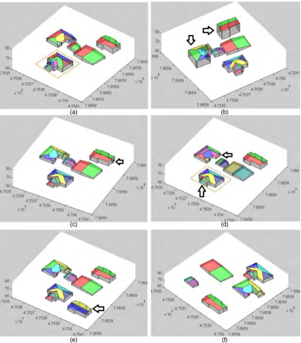
In this paper, 62 sets of changes have been made in the reference sites, AV(1)–(31) and HB(1)–(31), to evaluate the performance of the proposed building change detection method. Five test sites are used for visual demonstration, where two test sites of each reference site have the height changes in 2-D space, and the other three test sites of each reference site have changes in 2-D and/or 3-D spaces. In the first two test sites of the AV and HB reference sites, AV(17), AV(26), HB(17), and HB(26), the changes in building model are made in height, removal or addition of new verandas, addition of a new building, and relocation of three buildings. The other three test sites, i.e., AV(29)–(31) and HB(29)–(31),

are obtained by rotation of a building, destruction of a plane, and introduction of a new building in the building model.

As shown in Figures18and19, the changes in the reference sites are accurately detected by the proposed change detection method. For example, in Figures18b,c, and19b,c, the height change (in blue modified planes) are successfully detected by the proposed method. In addition, new veranda and new building planes (in red), demolished planes (in green), and unchanged planes (in yellow) are successfully detected from the building models of AV(17), AV(26), HB(17), and AV(26) sites. In the case of rotation of a building in Figures18d and19d and addition of a new building at the demolished building in Figures18e and19e, the modified planes (in blue), partially-modified planes (in cyan), demolished planes (in green), and unchanged planes (in yellow) are successfully detected by the proposed change detection method. In Figures18f and19f, a few building planes are removed from the building models of AV(31) and HB(31) sites, but these demolished planes (in green) and unchanged planes (in yellow) are also accurately detected by proposed change detection method.

Figure 18.Selected qualitative results of Aitkenvale (AV) reference site after applying the proposed change detection method: (a) AV reference models; and change detections in test sites: (b) AV(17); (c) AV(26); (d) AV(29); (e) AV(30); and (f) AV(31) (Table1). The reference models in (a) are shown in pink and grey colours. In the change detection results (b–f), the unchanged, new, modified, partially-modified and demolished planes are marked by yellow, red, blue, cyan and green colours, respectively.

Figure 19.Selected qualitative results of Hervey Bay (HB) reference site after applying the proposed change detection method: (a) HB reference models; and change detections in test sites: (b) HB(17); (c) HB(26); (d) HB(29); (e) HB(30); and (f) HB(31) (Table1). The reference models in (a) are shown in pink and grey colours. In the change detection results (b–f), the unchanged, new, modified, partially-modified and demolished planes are marked by yellow, red, blue, cyan and green colours, respectively.

7. Conclusions

Here, the building modelling task is performed in an unsupervised and data-driven fashion. Unlike the model-driven techniques, the roof types are not restricted to a pre-existing model catalogue. The roof planes, which are not extracted due to low point density, noise, and/or the vertical nature of the structures, are hypothesised using the roof topology assumption. As part of the modelling process, interrelations and interconnections among the building roof planes are used for the reconstruction of building models. It was demonstrated that the buildings at higher levels of detail are reconstructed by using individual roof planes and their interconnections based on their spatial adjacency.

The proposed 3-D change detection technique first defines the plane connections into three types of relations: parent-to-child, parent-to-parent and child-to-child. Then, it represents each generated building model into a graph-based data structure. Since, in practice, there are only a small number of buildings being changed in a period of time, the height difference values between the reference and the test models are initially used to find new, completely demolished and unchanged buildings. The corresponding building planes of these buildings are marked asnew,demolishedandunchanged. Thereafter, for only the modified building regions, the reference and building models are compared