Strongly Constrained Discrete Hashing

(1)

Chen, Y. and Tian, Z. and Zhang, H. and Wang, J. and Zhang, Dell

(2019) Strongly Constrained Discrete Hashing. IEEE Transactions on Image

Processing 29 , ISSN 1057-7149. (In Press)

Downloaded from:

Usage Guidelines:

Please refer to usage guidelines at

or alternatively

(2)

BIROn - Birkbeck Institutional Research Online

Chen, Y. and Tian, Z. and Zhang, H. and Wang, J. and Zhang, Dell

(2019) Strongly Constrained Discrete Hashing. IEEE Transactions on Image

Processing 29 , ISSN 1057-7149. (In Press)

Downloaded from:

Usage Guidelines:

Please refer to usage guidelines at

or alternatively

(3)

Strongly Constrained Discrete Hashing

Yong Chen, Zhibao Tian, Hui Zhang, Jun Wang, and Dell Zhang,

Senior Member, IEEE

Abstract—Learning to hash is a fundamental technique widely used in large-scale image retrieval. Most existing methods for learning to hash address the involved discrete optimization problem by the continuous relaxation of the binary constraint, which usually leads to large quantization errors and consequently suboptimal binary codes. A few discrete hashing methods have emerged recently. However, they either completely ignore some useful constraints (specifically the balance and decorrelation of hash bits) or just turn those constraints into regularizers that would make the optimization easier but less accurate. In this paper, we propose a novel supervised hashing method named Strongly Constrained Discrete Hashing (SCDH) which overcomes such limitations. It can learn the binary codes for all examples in the training set, and meanwhile obtain a hash function for unseen samples with the above mentioned constraints preserved. Although the model of SCDH is fairly sophisticated, we are able to find closed-form solutions to all of its optimization sub-problems and thus design an efficient algorithm that converges quickly. In addition, we extend SCDH to a kernelized version SCDHK. Our experiments on three large benchmark datasets

have demonstrated that not only can SCDH and SCDHK achieve

substantially higher MAP scores than state-of-the-art baselines, but they train much faster than those that are also supervised as well.

Index Terms—Learning to hash, image retrieval, discrete optimization.

I. INTRODUCTION

In this era of big data, there are more and more data that need to be stored, indexed, and processed automatically. Learning to hash, as a promising technique to represent data as compact binary codes for economical storage and efficient computation, has attracted much attention from many researchers as well as practitioners [2], [1], [3], [5], [6], [7], [8], [34]. To facilitate approximate nearest neighbors search, the binary codes should try to maintain the semantic similarity between any pair of samples in the data. The methods for learning to hash that preserve pairwise similarities in the learned binary Hamming space have already been shown to deliver impressive results in a number of applications, particularly large-scale image retrieval. Nevertheless, how to further improve the effectiveness and efficiency of such methods is still an important and challenging research problem today.

Generally speaking, there are two kinds of learning to hash methods: unsupervised and supervised. The latter usually works better than the former (due to the exploitation of the label Yong Chen is with the Key Lab of Machine Perception, School of EECS, Peking University, Beijing 100871, China.

Zhibao Tian and Hui Zhang are with the Department of Computer Science and Engineering, Beihang University, Beijing 100191, China.

Jun Wang is with the Department of Computer Science, University College London, London WC1E 6BT, U.K.

Dell Zhang is the corresponding author. He is with the Department of Computer Science and Information Systems, Birkbeck, University of London, London WC1E 7HX, and also with Blue Prism AI Labs, London WC2B 6NH, U.K. (e-mail: [email protected])

information) but can be considerably slower (due to the more sophisticated optimization algorithm needed).

In the unsupervised category, Spectral Hashing (SH) [9] first constructs the pairwise similarity matrix of the unla-beled data with a predefined kernel function and then solves the semantic hashing problem via spectral decomposition, which is quite inefficient when the dataset is large. Self-Taught Hashing (STH) [13] learns compact binary codes via relaxed SH from the unlabeled training documents and trains SVM classifiers to predict the binary codes for the testing documents. Similar to SH, the time-consuming spectral decomposition would make it impractical for large-scale real-world applications. Hashing with Graphs (AGH) [10] converts the pairwise similarity matrix into low-rank adjacency matrices by utilizing anchor graphs, which makes the corresponding optimization problem computationally feasible on large-scale image collections. However, the performance of image re-trieval using the produced binary codes is sensitive to the selection of anchors which is sometimes tricky. Scalable Graph Hashing (SGH) [12] utilizes feature transformation to approximate the whole pairwise similarity matrix efficiently and develops a sequential bit-by-bit learning algorithm, but the bit-wise optimization can be slow on large datasets particularly when the code length is long. All the above unsupervised learning to hash methods either make the continuous relaxation of the binary constraint or adopt just one of the discrete constraints to simplify the corresponding optimization problem, which leaves much room for improvement. Discrete Graph Hashing (DGH) [11] could be considered as an extension of AGH, which casts the graph-based hashing into a sophisticated discrete optimization framework. Although DGH also utilizes strong constraints as our proposed approach, due to the limitations of its optimization algorithm it often underperforms as we will show later in the experiments.

Semi-Supervised Hashing (SSH) [14] utilizes the class labels of data items to infer their semantic similarities/dissimilarities and then learn binary codes from them. Its eigen-decomposition based solution can be quite fast when the amount of avail-able labeled data is not very large. Minimal Loss Hashing (MLH) [15] models the semantic relationships among data items in the structural SVM framework in order to learn similarity-preserving binary codes. Supervised Hashing with Kernels (KSH) [16] exploits kernel-based hash functions to learn the binary codes which could represent complex nonlinear data. Fast Supervised Hashing with Decision Trees (FastH) [18] leverages the advantages of nonlinear functions over linear ones, and uses boosted decision trees to generate better binary codes. All the aforementioned supervised methods for learning to hash, along with other similar work [20], [19], [21], [22], [24], [25], face the same problem: when the labeled dataset is big, the corresponding pairwise similarity matrix would be

(4)

huge and therefore those methods will run very slowly and sometimes cannot finish in a reasonable time. Column Sampling Based Discrete Supervised Hashing (COSDISH) [26] is a fast algorithm using random partial labeled samples which can learn the binary codes for a large dataset with millions of images in just a dozen of seconds. However, the supervision information is not utilized to the fullest in this method, which restricts its effectiveness. Fast Scalable Supervised Hashing (FSSH) [44] combines pairwise and pointwise supervision signals in its discrete optimization algorithm which performs quite well for image retrieval, but the construction of the pairwise similarity matrix is quite space-inefficient and time-consuming. Notice that such supervised hashing methods usually have to ignore or drop some useful constraints (e.g., the balance and decorrelation of hash bits) in order to make the corresponding optimization problems easier to solve. Although recently, there emerges Discrete Proximal Linearized Minimization (DPLM) [46] and Binary Deep Neural Network (BDNN) [52] both of which start to take the balance and decorrelation constraints into account, they simply convert those constraints into parts of the objective function and thus make the optimization easier but less accurate.

There also exist some pairwise similarity based deep learning approaches to hashing [21], [42], [40], [43], [41]. Such deep-learning methods could achieve competitive performance, but they all would require massive training data and computational resources (with GPUs or TPUs), which makes them fairly expensive. In this paper, we focus on fast shallow models for learning to hash, which are cheap to run and practical for most large-scale real-world applications. How to reduce the cost of deep-learning based hashing is an open research problem, and we leave it for future work.

To unleash the full potential of supervised learning to hash, we propose a novel method named “Strongly Constrained Discrete Hashing (SCDH)”. Its main characteristics are sum-marized as follows.

• SCDH is a supervised discrete hashing method with complex constraints that not only require the hashing model yield binary codes but also enforce the balance and decorrelation of hash bits. Although the balance and decorrelation constraints have been shown to be crucially important for unsupervised learning to hash, they are typically absent in the existing supervised learning to hash methods because of the difficulty arising from discrete optimization.

• To address the tricky discrete optimization problem of SCDH, we introduce an auxiliary variable and decompose the original problem into several subproblems each of which has a closed-form solution. This makes the learning algorithm converge in just a small number of iterations (usually fewer than 10). Furthermore, we extend SCDH to a kernelized version dubbed “SCDHK” which could realize non-linear retrieval

functions for complex datasets.

• Extensive experiments on three large-scale image datasets have confirmed that our proposed methods could substantially outperform many state-of-the-art competitors with higher retrieval accuracies and meanwhile lower time costs. For example, on the NUS-WIDE dataset with 180k+ images, SCDH/SCDHK could be trained within a couple of minutes

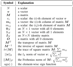
Table I: The notations adopted in this paper. Symbol Explanation

N a scalar

v a vector

M a matrix

vi a scalar: the (i)-th element of vectorv

mi a vector: the (i)-th column of matrixM

mij a scalar: the (ij)-th element of matrixM

0N anN×1vector with all0elements

1N anN×1vector with all1elements

IN anN×N identity matrix

O a matrix with all0elements

MT _{the transpose of matrix}_M

M−1 _{the inverse of square matrix}_M

tr(M) the trace of square matrixM:P

imii

||v||2 thel2 norm of vectorv: q

P

iv2i

||M||F the Frobenius norm ofM:

q P

ijm2ij

sgn(·) the element-wise sign function

using a commodity PC and achieve superior performance to the alternatives.

II. RELATEDWORK

From the perspective of optimization, the development of learning to hashing techniques could be roughly divided into three stages as follows.

Stage I: Hashing with spectral relaxation. The spectral

hashing (SH) [9] method, to the best of our knowledge, is probably the first to propose the balance and decorrelation constraints, in addition to the apparent binary constraint, for the task of learning to hash. The balance constraints require each bit to fire 50% of the time, while the decorrelation constraints require the bits to be uncorrelated. However, such a formulation implies an NP-hard mixed-integer optimization problem. To overcome this obstacle, SH chooses to relax the binary constraint into a continuous one during the learning of hash functions. Similarly, Self-Taught Hashing (STH) [13], Semi-Supervised Hashing (SSH) [14], Hashing with Graphs (AGH) [10] and Supervised Hashing with Kernels (KSH) [16] all belong to this family of spectral-based hashing methods in which the binary constraint is relaxed. This technique of continuous relaxation would greatly reduce the difficulty of optimization, but the solution could be suboptimal, i.e., the binary codes resulting from thresholding the continuous codes are likely to be inferior to those obtained by optimizing with the original binary constraint intact [17], [52]. Hence, to avoid such negative effects for hashing, our proposed SCDH/SCDHK

keeps the binary constraint discrete rather than relax them.

Stage II: Discrete hashing with the binary constraint

only.To make the discrete hashing problem tractable,

Super-vised Discrete Hashing (SDH) [17] does not make continuous relaxations but discard the “balance” and “decorrelation” constraints (employed in the above mentioned spectral-based hashing approaches), and thus develops the “discrete cyclic coordinate descent” (DCC) algorithm. Fast Supervised Discrete Hashing (FSDH) [45] enhances SDH using an exchangeable regression trick that leads to a closed-form solution for efficient binary codes. Fast Scalable Supervised Hashing (FSSH) [44]

(5)

differs from FSDH mainly in the utilization of both point-wise and pairpoint-wise labeled information; it can achieve better retrieval performance than FSDH that only leverages pointwise supervision. Column Sampling Based Discrete Supervised Hashing (COSDISH) [26] realizes binary hashing to handle large-scale image datasets by randomly sampling columns during the iterative learning process. To sum up, such kind of methods can avoid continuous relaxation and generate binary codes directly via discrete optimization algorithms. However, they have all ignored the desirable balance and decorrelation properties of hash bits, which would hurt the effectiveness of hashing. Compared with those methods, our SCDH/SCDHK

can also produce binary codes directly, and meanwhile try to satisfy the balance and decorrelation constraints.

Stage III: Discrete hashing with the other constraints too.As pointed out in SH [9], the balance and decorrelation constraints really help to maximize the compactness of binary codes. Recently, Discrete Proximal Linearized Minimization (DPLM) [46] and Binary Deep Neural Network (BDNN) [52] have been proposed to bring all those constraints (binary, bal-ance and decorrelaiton) together to achievestrongly constrained discrete hashing. However, what those methods actually do is to move the balance and decorrelation properties from the constraints to the objective function, i.e., treat them not as constraints but as regularizes instead. Although this is a popular trick for solving hard optimization problems approximately, it usually requires many iterations for the corresponding algo-rithms to converge. In contrast, our SCDH/SCDHK attempts to

findclosed-formsolutions to the strongly constrained optimiza-tion problem while maintaining both balance and decorrelaoptimiza-tion as constraints. Being able to getclosed-form solutions makes our algorithm much faster than the aforementioned iterative algorithms.

III. PROBLEMSTATEMENT

LetD={(xi,li)}Ni=1 be a set of images, wherexi∈RM

denotes the (i)-th image represented by an M-dimensional vector, andli∈ {0,1}C is its corresponding label vector, i.e., if imagexibelongs to thec-th class (c∈ {1,2,· · · , C}), then the c-th element of li is 1; otherwise, it is 0.N and C are the number of images and the number of classes in the dataset respectively. As in Ref. [39], the similaritysij betweenxiand

xj (i, j= 1,2,· · · , N) is calculated as: sij = 2 cos<li,lj >−1 = 2 l T ilj ||li||2· ||lj||2 −1 = 2 _l i ||li||2 T _l j ||lj||2 −1 . (1) If we further set: G= _l 1 ||l1||2 , l2 ||l2||2 ,· · · , lN ||lN||2 T , (2)

then the pairwise similarity matrix S = (sij)N×N could be

derived from the label information with:

S= 2GGT −1N1TN , (3)

where each elementsij would be in the range of[−1,+1]. We

aim to learn a set of hash functions that can preserve the label-based pairwise similarity in the Hamming space. Specifically,

K hash functions H(·)= [h1(·), h2(·),· · ·, hK(·)]T embed

each imagexiinto a K-bit binary code, i.e.,bi=H(xi)∈ {−1,+1}K_{, and then the whole dataset could be transformed}

intoB= [b1,b2,· · · ,bN]T ∈ {−1,+1}N×K. In principle, if

xiandxj share more class labels, then the Hamming distance between their corresponding binary codesbi andbj should be smaller. The mathematical notations used in this paper are summarized in TableI.

IV. PROPOSEDMETHOD

Here we describe in detail SCDH, a novel supervised discrete hashing method, in the joint learning framework where binary codes and hash functions are obtained simultaneously.

A. Similarity Preservation

Given a pair of images (xi,xj) each of which is encoded as aK-bit binary vector in the{−1,+1}K _{space, the value of}

their dot-product (which is in the range of[−K,+K]) should, ideally, be proportional to their semantic similaritysij. So we

make the binary codes preserve pairwise similarities through the following optimization:

min B ||K·S−BB T_||2 F (4) s.t.B∈ {−1,+1}N×K_,_BT₁ N =0K,BTB=N·IK ,

where the constraint BT1N =0K requires the hash bits to be

balanced(i.e., each bit fires 50% of the time) and the constraint

BTB = N ·IK requires the hash bits to be uncorrelated.

These two constrains, balance and decorrelation, are known to encourage the generation of compact binary codes [9], [11].

The objective function in (4) is quite common in supervised hashing with pairwise similarities preserved, but there exist two computational challenges: (1) how to construct theN×N

pairwise similarity matrixS efficiently; (2) how to solve the strongly constrained discrete optimization problem efficiently. In response to the first challenge, we represent S using the low-rank matrix G (in general C N) as shown in (3), which would significantly reduce the storage cost and also greatly accelerate the subsequent computation in the hashing process. With regard to the second challenge, most existing hashing methods (e.g., SH [9] and STH [13]) relax the discrete constraint B ∈ {−1,+1}N×K _{to a continuous one}

B∈RN×K, which simplifies the optimization but meanwhile

hurts the retrieval performance. Our solution, however, can afford to retain the discrete constraints with the help of an auxiliary variable, as explained below.

B. Joint Learning

Let X = [x1,x2,· · ·,xN]T. For fast image retrieval, we

use linear hash functionsP ∈RM×K to produce the binary

codes:

(6)

The hash functionsP can be learned simultaneously with the binary codes B by expanding (4) to the following:

min B,P||K·S−BB T_||2 F+λ||sgn(XP)−B|| 2 F+β||P|| 2 F (6) s.t.B∈ {−1,+1}N×K_,_BT₁ N =0K,BTB=N·IK ,

whereλis a positive parameter to weigh the relative importance of binary codes and hash functions, while β is a non-negative smoothing factor to prevent overfitting or irreversibility.

The sign function sgn(·)is not differentiable, which makes the optimization problem (6) difficult to solve directly. There-fore, we replacesgn(XP)with just XP. That is to say, we require each element ofXP itself rather than its sign to be as close as possible to the corresponding element of B (which is either+1or−1). Moreover, to make this discrete optimization problem easier, we introduce an auxiliary variable Z as an alias of B (i.e.,Z=B) and rewrite (6) as:

min B,P,Z||K·S−BZ T_||2 F+λ||XP −B|| 2 F +β||P|| 2 F (7) s.t. B∈ {−1,+1}N×K_, Z=B,ZT₁ N =0K,ZTZ=N·IK .

C. The Complete Optimization Problem

Finally, we go further to drop the constraint Z =B and make the relaxation thatZis a real-valued continuous variable approximating the discrete variable B. In other words,B and

Zare no longer required to be strictly identical but they should be similar to each other. Thus, the overall objective function that takes all the above considerations into account can be extended from (7) as follows:

min B,P,ZO(P, B, Z)=||K·S−BZ T_||2 F+ λ||XP −B||2 F+α||B−Z|| 2 F+β||P|| 2 F (8) s.t. B∈ {−1,+1}N×K_, Z∈RN×K,ZT1N =0K,ZTZ=N·IK. ,

where the additional parameter α controls how closely Z

approximatesB.

With the above joint learning framework, the binary codes for training data and the hash functions for out-of-sample data (e.g., testing samples, new query samples) can be obtained simultaneously. Given a set of out-of-sample imagesXoos, we

can encode them into binary codes using the hash functions:

Boos= sgn(XoosP), (9)

which is essentially a linear transformation and therefore can be computed very efficiently.

D. Kernelization

As demonstrated in KLSH [35], [36], KSH [16] and FastH [18], nonlinear hash functions can often perform much better than linear ones because of their ability of fitting complex patterns in the data. SCDH can also be extended to nonlinear hashing through kernel functions. Given a nonlinear mapping Φ : x ∈ RM 7→ Φ(x) ∈ RD (D could be

infinite), the entire image collection could be mapped into

Φ(X) ≡ [Φ(x1),Φ(x2),· · · ,Φ(xN)]T ∈ RN×D. Let us

randomly selectQanchors (i.e., a subset of images) from the image dataset, and denote them by y1,y2,· · · ,yQ; then we

can viewΦ(y1),Φ(y2),· · · ,Φ(yQ) as a set of base vectors

that can be used to represent any vector in RD. This is a

popular trick for handling big data and it usually works well in practice. Thus, we have:

Φ(P) =Φ([p1,p2,· · ·,pK])

= [Φ(y1),Φ(y2),· · · ,Φ(yQ)]A,

(10) whereA∈RQ×K. Accordingly, Eq. (5) is extended to:

B= sgn(Φ(X)Φ(P)) = sgn([Φ(x1),Φ(x2),· · ·,Φ(xN)] T [Φ(y1),Φ(y2),· · ·,Φ(yQ)]A) = sgn (Φ(xi)TΦ(yj))N×QA . (11)

Let K : RD × RD 7→ R denote the kernel function

corresponding to the nonlinear mapping Φ and KQ ≡ (Φ(xi)TΦ(yj))N×Q the kernel matrix. Similar to (8), the

kernelized version of SCDH is formulated as: min B,A,Z||K·S−BZ T_||2 F+λ||KQA−B||2F +α||B−Z||2 F+β||A||2F (12) s.t. B∈ {−1,+1}N×K_, Z∈RN×K,ZT1N =0K,ZTZ=N·IK. ,

which is called SCDHK for short.

After the kernel functionK being chosen and the matrixA

being learned, an out-of-sample image xoos can be encoded:

boos= sgn h (Φ(xoos) T Φ(yj))₁_×_QA iT = sgn _h (K(xoos,yj))₁_×_QA iT . (13)

The vector-matrix multiplication involved in the above equation should be quite computationally efficient, as usually QN.

V. OPTIMIZATION

In this section, we explain how the intricate optimization problem of the above SCDH method can be solved efficiently. The solution to SCDHK is very similar, so it is omitted here.

The optimization problem (8) has three variables to be optimized: P, B and Z. Our algorithm is to update each variable while holding the other two fixed (i.e., alternating minimization), and iterate this process until convergence.

A. Update P withB andZ Fixed

When B andZ are fixed, the objective function ofP is given by: min P O(P)=λ||XP −B|| 2 F+β||P|| 2 F, (14)

which is in fact a least-squares problem with L2regularization. Setting ∂O_∂(_PP) =O, we get the closed-form solution:

P = XTX+β λIM −1 XTB. (15)

(7)

B. Update B withZ andP Fixed

When P andZ are fixed, the objective function ofB is simplified into: min B O(B)=||K·S−BZ T_||2 F+ λ||XP −B||2 F+α||B−Z|| 2 F (16) s.t.B∈ {−1,+1}N×K .

This is equivalent to the optimization problem: max

B tr(B

T_{_K_·_SZ₊_λ_XP ₊_α_Z_}₎ ₍₁₇₎

s.t.B∈ {−1,+1}N×K

which can be solved by applying the following theorem.

Theorem 1. Given a matrix C ∈ _RN×K_{, the optimization}

problem

max

B tr(BC

T₎ _s_._t_._B

∈ {−1,+1}N×K, (18)

has the closed-form solution B= sgn(C).

Proof. According to the definition of the trace function,

tr(BCT) =X

i,jbijcij . (19)

So the optimization problem (18) is the same as: max

bij

bijcij s.t. bij ∈ {−1,+1} , (20)

for each bij with i ∈ {1,2,· · ·, N}, j ∈ {1,2,· · ·, K}.

Obviously, to achieve the maximum, each bijcij needs to be

positive, i.e.,bij=sgn(cij). Q.E.D.

Thus, the closed-form solution of (16) is given by:

B= sgn(K·SZ+λXP +αZ). (21)

C. Update Z withP and B Fixed

When P andB are fixed, the objective function of Z is written as: min Z O(Z)=||K·S−BZ T_||2 F+α||B−Z|| 2 F (22) s.t.Z∈RN×K,ZT1N =0K,ZTZ=N·IK .

It can be further reduced to: max

Z tr(Z

T

{K·SB+αB}) (23) s.t.Z∈RN×K,ZT1N =0K,ZTZ=N·IK .

LetE=K·SB+αB, and then we can get the closed-form solution through the following theorem.

Theorem 2. The optimization problem

max Z tr(Z

T_E₎ _s_._t_._ZT₁

N =0K,ZTZ=N·IK , (24)

has the closed-form solution:

Z=√N[U,U¯][V,V¯]T . (25)

The matrices

U = [u1,u2,· · · ,uK0]and V = [v₁,v₂,· · · ,v_K0]

are obtained via the Singular Value Decomposition (SVD) of J E withJ =IN−N11N1TN, i.e., J E=UΣVT =XK 0 k=1σkukv T k . (26) Note thatσ1≥σ2≥ · · · ≥σK0 >0.

Then, the matrices U¯ ∈ RN×(K−K

0₎

and V¯ ∈RK×(K−K

0₎

are obtained via the Gram-Schmidt process such that ¯

UTU¯ = IK−K0, [U,1_N]TU¯ = O, V¯TV¯ = I_K₋_K0, and

VT_V_¯ ₌_{O. If} _K0 ₌_K_,_U¯ _and _V¯ _{will be empty.} Proof. Please refer to Ref. [11].

D. Computational Complexity

The learning algorithm for SCDH is built on top of the above three subproblems of optimization and formally specified in Algorithm 1. In each iteration, three closed-form solutions — Eqs. (15), (21) and (25) — need to be computed for the three corresponding subproblems respectively.

Regarding theP-subproblem, the main computational oper-ations are the multiplicoper-ations ofXTX and the inverse of a

M×M square matrix whose time complexities areO(N M2₎ andO(M3₎_{respectively. The whole time complexity of this} subproblem is O(N M2₊_M3₊_{N M K}₊_KM2₎_{, where}_M is the number of original features andK is the length of hash codes. Usually M, K N (the number of samples in the dataset), which makes the time complexity of this subproblem linear w.r.t.N.

Regarding theB-subproblem, the most time-consuming part is the computation of SZ. However, due to the fact that S= 2GGT−1N1TN, the time complexity could be reduced from O(KN2)toO(CKN), whereCis the number of class labels (CN). Thus, the whole time complexity of this subproblem isO(CKN+KM N), which is linear w.r.t.N.

Regarding the Z-subproblem, the main step requiring intensive computation is the SVD for aN×K matrix whose time complexity is O(N K2₎_{. It is easy to see that the other} operations would require less expenditure of time than this. Therefore, we can conclude that the whole time complexity of this subproblem is also linear w.r.t.N.

Algorithm 1: SCDH

Input:Data matrix X, label matrixG, length of hash

codesK, hyperparameters α,β andλ, max iterationsmaxIter, precisionε.

Output: Binary codesB, auxiliary variable Z and

hash functionsP. 1 Randomly initializeP,B, andZ;

2 whilenot convergent do

/* Convergence: the number of

iterations is bigger than maxIter,

or the error is less than ε. */

3 OptimizeP according to Eq. (15); 4 OptimizeB according to Eq. (21); 5 OptimizeZ according to Eq. (25); 6 end

(8)

In summary, the total computational complexity of the entire SCDH algorithm is linear w.r.t. N for each iteration. Moreover, in practice, the algorithm usually needs only a few (<10) iterations to reach convergence (see Fig.1). Hence, the proposed SCDH method is indeed highly efficient.

VI. EXPERIMENTS

We have used several large-scale image datasets to evaluate SCDH’s retrieval performance on a PC with Intel(R) Xeon(R) CPU E5-2650 v4 @2.20GHz and 64GB RAM.

A. Datasets

Caltech256 contains 30,607 images belonging to 256

cate-gories [27]. Each image is represented by a 1,024-dimension CNN feature vector associated with one category label. We randomly select 26,000 samples for training and 3,000 samples for testing (i.e., Train:Test=26,000:3,000).

Cifar10 includes 60,000 color images (of size 32×32) that

are divided evenly into 10 classes (each of which holds 6,000 samples) [28]. We choose 5,400 samples from each class as the training set and the remaining as the testing set (i.e., Train:Test=54,000:6,000). For each image, a 512-dimension GIST feature vector is extracted as its representation.

NUS-WIDE is a real-world web database originally

con-taining 269,648 images each associated with multiple textual tags [37]. Following the protocol in Ref. [38], we focus on 186,577 images that cover the top-10 most frequent semantic concepts. In our experiments, we take 1% of the dataset as the testing set and the remaining as the training set (i.e., Train:Test=184,711:1,866). Each image is converted into a 500-dimensional bag-of-visual-word features. This is a relatively larger and more challenging dataset for image retrieval.

B. Evaluation

In the retrieval experiments, those images sharing at least one class label or tag with the query image would be considered as relevant results. Mean Average Precision (MAP) is a very popular metric for evaluating the retrieval performance of learning to hash methods [31], [32], [30], [18], [26], [24]. For all our experiments on the above mentioned image datasets, we would also employ MAP as the measure of effectiveness. Besides, the running time of each method in the experiments would also be recorded to assess its efficiency.

Regarding the baseline methods for comparison, we have chosen the most representative as well as the currently most competitive ones: LSH1_[₂_{], PCAH}2_[₃₁_{], ITQ (rotation after}

PCA for binary codes)3_[₃_{], DGH}4_[₁₁_{], SGH}5_[₁₂_],

CCA-ITQ6_[₃_{], SDH}7_[₁₇_{], HC-SDH}4_[₂₃_{], FSDH}8_[₄₅_{], FastH}9_[₁₈_],

1_{http://www.cad.zju.edu.cn/home/dengcai/Data/DSH.html}

2_{http://www.cad.zju.edu.cn/home/dengcai/Data/DimensionReduction.html} 3_{https://goo.gl/AGuu86}

4_{Our own implementation of this algorithm in MATLAB.} 5_{http://cs.nju.edu.cn/lwj/L2H.html}

6_{https://github.com/jfeng10/ITQ-image-retrieval} 7_{https://github.com/bd622/DiscretHashing} 8_{https://tongliang-liu.github.io/publications.html} 9_{https://bitbucket.org/chhshen/fasthash/src/master/}

COSDISH5[26], FSSH10[44]. These 12 competitors in our experiments come from two groups: the first5are unsupervised methods which usually run fast but may yield inferior results; whereas the other 7 are supervised methods which often produce high MAPs for image retrieval though their training speed could be slow. Among them, HC-SDH has just been evaluated on Cifar10 due to some of its limitations (e.g.,

K ≥ C and single-label only); the other baseline methods can successfully run on at least two of the three image datasets mentioned earlier. There also exist many other learning to hash methods such as SH [9] and KSH [16] which perform well on small datasets but cannot scale to big datasets and therefore have to be excluded from the experiments.

C. Settings

All the baseline methods except DGH and HC-SDH have already been implemented in MATLAB with their source codes provided by the corresponding authors. To ensure a fair comparison (especially for the speed), we have also implemented DGH and HC-SDH as well as our proposed approaches SCDH/SCDHK in MATLAB. The inputs (i.e., the

data and label matrices) to all the different methods are identical. The initialization of each baseline method is carried out in exactly the same way as described in its original paper. The hyperparameters of each method have been tuned on different datasets to get the best validation performance, in accordance with the authors’ proposals.

For our proposed method SCDH, we set maxIter = 10 andε= 10−10 in Algorithm1. Note that our method usually converges in fewer than10iterations in the experiments (see Fig.1). For the hyperparametersα,β andλ, we have tuned them by grid search with each of them ranging from 10−9 to 109_{. SCDH would be able to achieve good MAP scores} using most of the parameter values within the above range, and the finally chosen combination is (α= 0.1,β = 1, λ= 10). This set of hyperparameters would be directly adopted by the kernelized version of our method SCDHK in our experiments.

SCDHK would employ the Gaussian (RBF) kernelK(x,y) =

exp(−||x−y||2

2/(2σ2))withσ= 0.4 and make use of 2,000 anchors (see SectionVI-Ffor further details).

D. Results

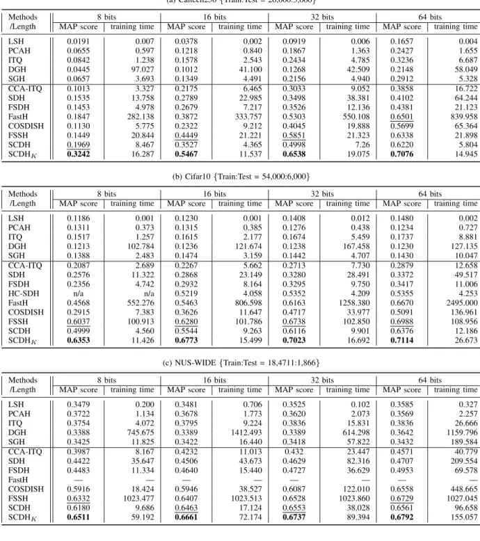
TableIIshows the MAP scores and the training time costs11

of our proposed approaches as well as the baseline methods on three different image datasets. The code length has been set to 8,16,32, and64bits.

Unsurprisingly, the experimental results indicate that the supervised hashing methods outperform the unsupervised ones, though they are usually slower. This is consistent with our intuition and previous research findings that exploiting the label information can in general enhance the effectiveness of hashing.

Among the supervised hashing methods, our proposed SCDHK always delivers the best performance, while most

10_{https://lcbwlx.wixsite.com/fssh}

11_{Compared with the training time costs, the testing time costs can usually} be ignored, especially on large datasets.

(9)

Table II: The MAP scores and training time costs (in seconds) of different hashing methods. The best results are in bold, the second-best are underlined, and “—” means that the method was unable to finish in a reasonable time.

(a) Caltech256{Train:Test = 26,000:3,000}

Methods /Length

8 bits 16 bits 32 bits 64 bits

MAP score training time MAP score training time MAP score training time MAP score training time

LSH 0.0191 0.007 0.0378 0.002 0.0919 0.006 0.1657 0.004 PCAH 0.0655 0.597 0.1218 0.840 0.1867 1.363 0.2427 1.655 ITQ 0.0842 1.238 0.1578 2.543 0.2434 4.785 0.3236 6.687 DGH 0.0445 97.027 0.1012 41.100 0.1268 42.509 0.2148 58.049 SGH 0.0657 3.693 0.1349 4.491 0.2156 4.940 0.2912 5.328 CCA-ITQ 0.1013 3.327 0.2175 6.465 0.3033 9.052 0.3858 16.722 SDH 0.1535 13.758 0.2789 22.985 0.3498 38.381 0.4102 64.244 FSDH 0.1453 4.978 0.2679 7.217 0.3526 12.136 0.4381 21.123 FastH 0.1847 282.138 0.3872 333.757 0.5303 550.108 0.6501 839.958 COSDISH 0.1130 5.775 0.2322 9.212 0.4045 19.888 0.5699 65.364 FSSH 0.1449 20.844 0.4449 21.221 0.5851 21.323 0.6338 21.898 SCDH 0.1969 8.467 0.3527 4.365 0.4998 7.26 0.6220 5.804 SCDHK 0.3242 16.287 0.5467 11.537 0.6538 19.075 0.7076 14.945 (b) Cifar10{Train:Test = 54,000:6,000} Methods /Length

LSH 0.1186 0.001 0.1230 0.001 0.1408 0.012 0.1480 0.002 PCAH 0.1311 0.373 0.1315 0.385 0.1276 0.438 0.1234 0.727 ITQ 0.1517 1.257 0.1615 2.177 0.1674 5.459 0.1737 8.881 DGH 0.1213 102.784 0.1236 121.674 0.1238 167.458 0.1230 127.135 SGH 0.1388 2.483 0.1474 3.159 0.1442 4.707 0.1430 10.047 CCA-ITQ 0.2087 2.689 0.2267 5.662 0.2713 7.730 0.2879 12.658 SDH 0.2576 11.322 0.2868 23.149 0.3280 28.491 0.3372 49.517 FSDH 0.2356 4.742 0.2932 8.164 0.3295 9.750 0.3417 11.006 HC-SDH n/a n/a 0.5219 4.058 0.5352 4.209 0.5355 4.253 FastH 0.4568 552.276 0.5463 806.598 0.6163 1258.380 0.6670 2495.000 COSDISH 0.2915 7.383 0.3626 11.647 0.4717 33.977 0.5091 136.961 FSSH 0.6037 100.913 0.6280 101.786 0.6738 102.850 0.6988 108.956 SCDH 0.4999 4.560 0.5544 9.263 0.6116 9.901 0.6376 12.186 SCDHK 0.6353 11.426 0.6773 15.499 0.7023 16.692 0.7114 26.673 (c) NUS-WIDE{Train:Test = 18,4711:1,866} Methods /Length

LSH 0.3479 0.200 0.3481 0.706 0.3525 0.102 0.3585 0.327 PCAH 0.3722 1.134 0.3678 1.773 0.3620 2.073 0.3569 2.257 ITQ 0.3754 4.072 0.3795 9.224 0.3836 15.831 0.3836 26.666 DGH 0.3388 745.675 0.3389 1412.493 0.3389 614.298 0.3642 1159.796 SGH 0.3425 11.825 0.3422 16.440 0.3418 57.822 0.3432 189.584 CCA-ITQ 0.3987 8.167 0.4232 11.013 0.432 23.447 0.4571 40.779 SDH 0.4422 35.647 0.4506 43.673 0.4629 82.316 0.4707 209.554 FSDH 0.4483 11.334 0.4640 15.440 0.4727 36.629 0.4953 69.578 FastH — — — — — — — — COSDISH 0.5916 18.424 0.5946 38.527 0.6087 122.010 0.6558 448.665 FSSH 0.6332 1023.477 0.6407 1023.513 0.6528 1023.860 0.6729 1027.045 SCDH 0.6180 9.686 0.6463 17.124 0.6553 38.028 0.6561 96.658 SCDHK 0.6511 59.192 0.6661 72.174 0.6737 89.394 0.6792 155.057

of the time SCDH and FSSH compete for the second spot. SCDHK’s noticeable performance gain over the vanilla SCDH

confirms the usefulness of nonlinear hash functions for large and complex datasets. Although FastH sometimes provides slightly higher MAP scores than SCDH, it is much more time-consuming, especially with longer binary codes and larger image collections. In fact, FastH was not able to finish the experiments on NUS-WIDE, the largest dataset, in a reasonable time. SDH, a pointwise hashing method, does not really preform better than the pairwise similarity preservation

based methods like SCDH/SCDHK in terms of MAP scores;

it is also much slower than our methods in most cases. Although FSDH, an extension of SDH, exhibits a slightly faster training speed than SCDH/SCDHK, its retrieval effectiveness

is a lot worse. Moreover, HC-SDH which incorporates the balance and decorrelation constraints into SDH by Hadamard operations [23] works significantly better than SDH and FSDH, which confirms the merit of imposing such constraints for hashing. However, HC-SDH’s retrieval performance still lags far behind that of our proposed SCDH/SCDHK.

(10)

0 5 10 15 20 0.96 0.965 0.97 0.975 0.98 0.985 0.99 0.995 1 iterations

Normalized Objective Function Value

Caltech256 Cifar10 NUS−WIDE (a) 32 bits 0 5 10 15 20 0.97 0.975 0.98 0.985 0.99 0.995 1 iterations

Normalized Objective Function Value

Caltech256 Cifar10 NUS−WIDE

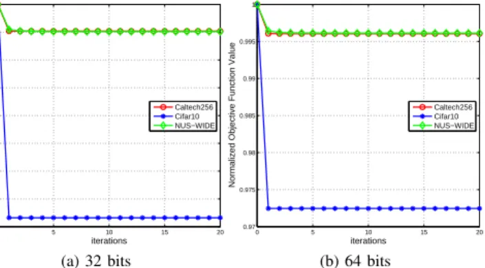
(b) 64 bits Figure 1: The convergence curves of SCDH.

Similar to SCDHK, some baseline methods (i.e., SGH,

FSDH, HC-SDH and FSSH) also use the kernel trick to achieve nonlinear hashing12_{. FSSH evidently reaches the best retrieval}

performance among the baseline methods, but it is consistently inferior to SCDHK in terms of both MAP scores and training

speeds on all the three datasets, which testifies the effectiveness and efficiency of our proposed methods. Specifically, FSSH utilizes both pairwise and pointwise supervision for hashing, while SCDHK is based entirely on pairwise similarity

preser-vation. The advantages of SCDHK against FSSH probably

come from the two strong constraints, i.e., the balance and decorrelation of hash bits (see SectionVI-Gfor a more detailed analysis of their usefulness).

E. Convergence Analysis

It is clear from Algorithm1for SCDH that the value of the objective function O(P, B, Z)will decrease from iteration to iteration until it is stabilized:

O(Pt,Bt,Zt)≥O(Pt+1,Bt,Zt) ≥O(Pt+1,Bt+1,Zt) ≥O(Pt+1,Bt+1,Zt+1).

(27)

Since during the execution of the algorithm, the objective function can only go down and it cannot go lower than zero, the iterative algorithm for SCDH is theoretically guaranteed to converge.

Let us further investigate how fast the algorithm can converge. Fig. 1 shows the convergence curves of SCDH on all those three large datasets for 32-bit and 64-bit codes13_{. In each}

sub-graph thex-axis represents the iteration number and they-axis represents the normalized14 _{value of the objective function. It}

is obvious that the SCDH algorithm converges very quickly within just a few iterations. This is probably attributed to the low-rank representations for the pairwise similarity matrix 12_{For a fair comparison, in our experiments, all those nonlinear hashing} methods make use of the Gaussian kernel equipped with 2000 anchors, except that SGH uses 300 anchors only (as that leads to comparable MAP scores but much less training time).

13_{The convergence curves of SCDH for other code lengths show the same} trend and therefore are omitted.

14_{To normalize the value of the objective function at each iteration, it is} divided by its maximum value (which is always received at the first iteration).

Table III: The MAP scores of SCDHK with different kernels.

kernels Cifar10 NUS-WIDE

Linear 0.6255 0.6279 0.6436 0.6443

Polynomial (α=1,c=0,d=8) 0.6967 0.7255 0.6524 0.6794 Laplacian (σ=0.4) 0.6655 0.6811 0.6615 0.6726 Sigmoid (γ=0.7,c=0) 0.6670 0.7036 0.6726 0.6854 Gaussian (σ=0.4) 0.7023 0.7114 0.6737 0.6792

and the efficient closed-form solutions to the subproblems of optimization.

The convergence of SCDHK is similar to that of SCDH, so

its analysis is omitted here.

F. Hyperparameters of SCDHK

SCDHK (with the Gaussian kernel) has two essential

hyperparameters: the number of randomly selected anchorsQ

and the kernel bandwidthσ.

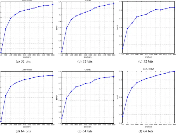
Keeping all the other parameters fixed, we vary the number of anchorsQfrom 100 to 8,000 and plot the retrieval performance of SCDHK in Fig.2. It can be observed on all the datasets that

along with the increase ofQ, SCDHK’s MAP scores would get

higher and higher. This is reasonable because a certain number of basis vectors (anchors) would be necessary to represent complex data samples well. However, we can also see that as

Qbecomes bigger, the performance gain is diminishing and the training time cost is rising. Throughout our experiments, Qis set to 2,000 which enables SCDHK to beat the state-of-the-art

methods while being able to finish within just a couple of minutes on all the datasets.

Keeping all the other parameters fixed, we vary the kernel bandwidth σ from 0.01 to 100 and plot the retrieval perfor-mance of SCDHK in Fig.3. As can be seen clearly, SCDHK

performs well on all the datasets whenσis between 0.3 and 1.0, though its optimal value for each dataset is slightly different from one another. Throughout our experiments,σis set to 0.4 which can provide decent MAP scores across different datasets.

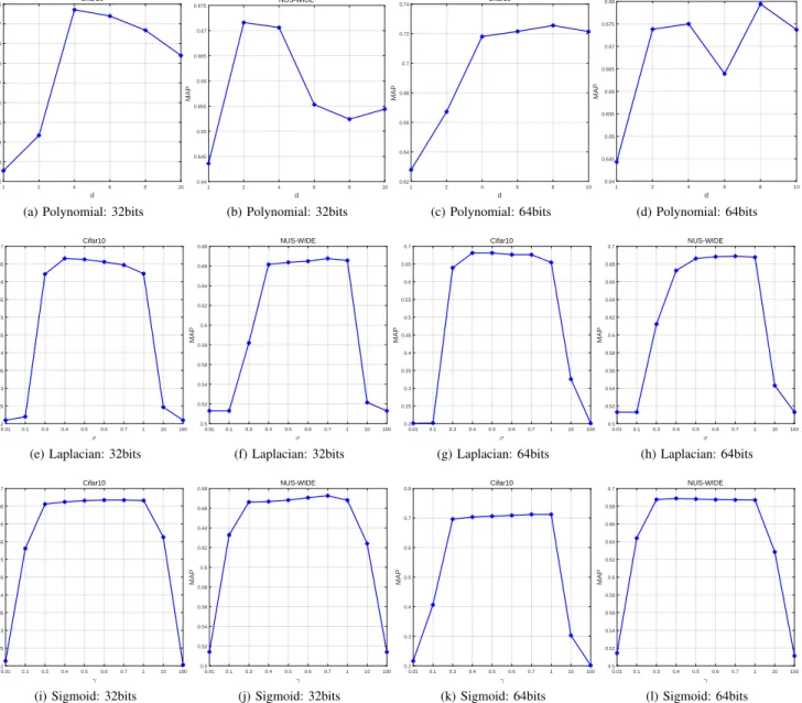
Furthermore, we explore the possibility of using different kernels other than the default Gaussian kernel in SCDHK.

Specifically, the popular kernels including linear, polyno-mial [47], Laplacian [48], Sigmoid [50] and Gaussian [51] as listed below have been compared empirically.

• Linear kernel:K(x,y) =xT_y _;

• Polynomial kernel:K(x,y) = αxT_y₊_cd

;

• Laplacian kernel:K(x,y) = exp−||x₂−_σy||;

• Sigmoid kernel:K(x,y) = tanh γxTy+c; • Gaussian kernel:K(x,y) = exp−||x₂−_σy2||2

.

In our study, the kernel hyperparameters αand c are set to their default values 1 and 0 respectively15_{; the kernel}

hyperpa-rametersd,σandγ are tuned for their corresponding kernel functions, as shown in Fig.4 and Fig.3. The hyperparameter tuning curves for Laplacian, Sigmoid and Gaussian kernels exhibit similar patterns, while the polynomial kernel looks not 15_{We have also tried using many other values for}_α_and_c_{, but their best} results are similar to those using the default values.

(11)

100 500 100015002000250030004000 5000600070008000 0.25 0.3 0.35 0.4 0.45 0.5 0.55 0.6 0.65 0.7 0.75 anchors MAP Caltech256 (a) 32 bits 100 500 1000150020002500 300040005000600070008000 0.58 0.6 0.62 0.64 0.66 0.68 0.7 0.72 0.74 anchors MAP Cifar10 (b) 32 bits 100 500 1000150020002500300040005000 600070008000 0.63 0.64 0.65 0.66 0.67 0.68 0.69 anchors MAP NUS−WIDE (c) 32 bits 100 500 100015002000250030004000 5000600070008000 0.35 0.4 0.45 0.5 0.55 0.6 0.65 0.7 0.75 0.8 anchors MAP Caltech256 (d) 64 bits 100 500 1000150020002500 300040005000600070008000 0.58 0.6 0.62 0.64 0.66 0.68 0.7 0.72 0.74 0.76 anchors MAP Cifar10 (e) 64 bits 100 500 1000150020002500300040005000 600070008000 0.63 0.64 0.65 0.66 0.67 0.68 0.69 anchors MAP NUS−WIDE (f) 64 bits Figure 2: The MAP scores of SCDHK (Gaussian kernel) w.r.t. the number of anchors Q.

Table IV: The MAP scores of SCDHK with the constraints

turned on (“_X”) or off (“×”).

balance decorrelation Cifar10 NUS-WIDE 32 bits 64 bits 32 bits 64 bits

× × 0.6504 0.6795 0.6001 0.6171

X × 0.6571 0.6869 0.6351 0.6586

× X 0.6607 0.6816 0.6603 0.6751

X X 0.7023 0.7114 0.6737 0.6792

so stable. Accordingly, the best performances that could be achieved by these different kernels are summarized in TableIII. It can be seen that (i) all the nonlinear kernels work apparently better than the linear kernel, and (ii) the nonlinear kernels produce somewhat similar performances. Overall, the Gaussian kernel (which has only one hyperparameter σ) seems to be slightly superior to the other kernels in terms of MAP scores. It is the kernel of choice for many nonlinear hashing methods such as KSH [16], SGH [12], FSDH [45], FSSH [44], and also our own SCDHK.

G. Ablation Study

To investigate the contributions of the “balance” constraint (BT1N =0K) and the “decorrelation” constraint (BTB= N·IK) to our proposed SCDHK, we conduct ablation study,

i.e., we drop either constraint or both from SCDHK and solve

the modified optimization problem. The results on Cifar10

Table V: Retrieval performance: SCDHK vs. DPLM.

Methods/Length 32 bits 64 bits

MAP score training time MAP score training time Cifar10 DPLM 0.6671 17.903 0.6889 29.377 SCDHK 0.7023 16.692 0.7114 26.673 NUS-WIDE DPLM 0.6703 95.792 0.6782 170.471 SCDHK 0.6737 89.394 0.6792 155.057

and NUS-WIDE are collected in TableIV, from which some observations can be made.

• Using either constraint would be better than using neither of them, which means that they are both helpful.

• Between these two constraints, “decorrelation” seems to be more important than “balance” in the sense of providing more performance gains.

• Combining these two constraints would make the hashing method benefit from both of them and thus generate the best results.

To summarize, the “balance” and “decorrelation” constraints which have often been ignored due to the optimization difficulty, can indeed make great improvements to hashing for large-scale image retrieval.

H. Constraints vs. Regularizers

Recall that the proposed SCDHK model (12) has been

(12)

sub-0.010 0.1 0.3 0.4 0.5 0.6 0.7 1 10 100 0.1 0.2 0.3 0.4 0.5 0.6 0.7 σ MAP Caltech256 (a) 32 bits 0.01 0.1 0.3 0.4 0.5 0.6 0.7 1 10 100 0.2 0.25 0.3 0.35 0.4 0.45 0.5 0.55 0.6 0.65 σ MAP Cifar10 (b) 32 bits 0.01 0.1 0.3 0.4 0.5 0.6 0.7 1 10 100 0.5 0.52 0.54 0.56 0.58 0.6 0.62 0.64 0.66 0.68 σ MAP NUS−WIDE (c) 32 bits 0.01 0.1 0.3 0.4 0.5 0.6 0.7 1 10 100 0 0.1 0.2 0.3 0.4 0.5 0.6 0.7 0.8 σ M A P Caltech256 (d) 64 bits 0.01 0.1 0.3 0.4 0.5 0.6 0.7 1 10 100 0.2 0.3 0.4 0.5 0.6 0.7 0.8 0.9 σ MAP Cifar10 (e) 64 bits 0.01 0.1 0.3 0.4 0.5 0.6 0.7 1 10 100 0.5 0.52 0.54 0.56 0.58 0.6 0.62 0.64 0.66 0.68 0.7 σ MAP NUS−WIDE (f) 64 bits Figure 3: The MAP scores of SCDHK (Gaussian kernel) w.r.t. the kernel bandwidthσ.

problem of optimization. Actually, it is also possible to tackle this optimization problem by converting the hard “balance” and “decorrelation” constraints into two extra regularizers in the objective function, as in DPLM [46]. To further understand those two different ways of incorporating “balance” and “decorrelation” into hashing, we make empirical comparisons between our SCDHK (that uses hard constraints) and DPLM

(that uses soft regularizers). For SCDHK, the hyperparameter

settings have been explained in Sections VI-CandVI-F. For DPLM, the hyperparameters have been tuned to get the best possible performance. As shown in Table V, SCDHK has

not only higher MAP scores but also lower time costs than DPLM, on both Cifar10 and NUS-WIDE. It turns out that we do not really have to sacrifice effectiveness for efficiency (by converting those two strong constraints into regularizers), thanks to our Algorithm1 based on closed-form solutions.

I. Shallow vs. Deep

This paper mainly focuses on exploiting the “balance” and “decorrelation” constraints in the hashing methods that are not based on deep learning (which typically require enormous computing power like GPU clusters). Nevertheless, we are curious about how our proposed SCDH/SCDHK would

compete against the so-called deep hashing methods that have emerged in the last few years, such as DeepBit [55], [56], SADH [57], and DPSH [21]. TableVIshows the comparison between such deep hashing methods and the shallow hashing method SCDH/SCDHK on Cifar10 and NUS-WIDE. It is

Table VI: Retrieval performance: SCDH(K) vs. Deep Hashing.

MAP score training time MAP score training time Cifar10 DeepBit 0.1875 7731.449 0.1969 9671.132 SADH 0.3147 9150.755 0.3308 10981.705 DPSH 0.7037 10795.150 0.7261 12946.728 SCDH 0.6116 9.901 0.6376 5.888 SCDHK 0.7023 16.692 0.7114 12.407 NUS-WIDE DeepBit 0.4092 12211.901 0.4203 14903.540 SADH 0.4564 15462.948 0.4732 19432.642 DPSH 0.7275 16397.246 0.7383 19390.623 SCDH 0.6553 38.028 0.6561 96.658 SCDHK 0.6737 89.394 0.6792 155.057

obvious that all the deep hashing methods are several orders of magnitude slower than SCDH/SCDHK. Moreover, the two

deep hashing methods DeepBit and SADH actually get lower MAP scores than SCDH/SCDHK, which is probably because

they are unsupervised while SCDH/SCDHK is supervised.

The deep hashing method DPSH which is supervised does outperform SCDH/SCDHK in terms of MAP scores, though it

requires significantly more training time than SCDH/SCDHK.

This demonstrates the superior ability of deep neural networks in fitting complex data. It may be possible to utilize a deep neural network instead of the kernel trick to enable SCDH for nonlinear hashing, which is a research problem to be investigated in the future.

(13)

1 2 4 6 8 10 d 0.62 0.63 0.64 0.65 0.66 0.67 0.68 0.69 0.7 0.71 MAP Cifar10

(a) Polynomial: 32bits

1 2 4 6 8 10 d 0.64 0.645 0.65 0.655 0.66 0.665 0.67 0.675 MAP NUS-WIDE (b) Polynomial: 32bits 1 2 4 6 8 10 d 0.62 0.64 0.66 0.68 0.7 0.72 0.74 MAP Cifar10 (c) Polynomial: 64bits 1 2 4 6 8 10 d 0.64 0.645 0.65 0.655 0.66 0.665 0.67 0.675 0.68 MAP NUS-WIDE (d) Polynomial: 64bits 0.01 0.1 0.3 0.4 0.5 0.6 0.7 1 10 100 0.2 0.25 0.3 0.35 0.4 0.45 0.5 0.55 0.6 0.65 0.7 MAP Cifar10

(e) Laplacian: 32bits

0.01 0.1 0.3 0.4 0.5 0.6 0.7 1 10 100 0.5 0.52 0.54 0.56 0.58 0.6 0.62 0.64 0.66 0.68 MAP NUS-WIDE (f) Laplacian: 32bits 0.01 0.1 0.3 0.4 0.5 0.6 0.7 1 10 100 0.2 0.25 0.3 0.35 0.4 0.45 0.5 0.55 0.6 0.65 0.7 MAP Cifar10 (g) Laplacian: 64bits 0.01 0.1 0.3 0.4 0.5 0.6 0.7 1 10 100 0.5 0.52 0.54 0.56 0.58 0.6 0.62 0.64 0.66 0.68 0.7 MAP NUS-WIDE (h) Laplacian: 64bits 0.01 0.1 0.3 0.4 0.5 0.6 0.7 1 10 100 0.2 0.25 0.3 0.35 0.4 0.45 0.5 0.55 0.6 0.65 0.7 MAP Cifar10

(i) Sigmoid: 32bits

0.01 0.1 0.3 0.4 0.5 0.6 0.7 1 10 100 0.5 0.52 0.54 0.56 0.58 0.6 0.62 0.64 0.66 0.68 MAP NUS-WIDE (j) Sigmoid: 32bits 0.01 0.1 0.3 0.4 0.5 0.6 0.7 1 10 100 0.2 0.3 0.4 0.5 0.6 0.7 0.8 MAP Cifar10 (k) Sigmoid: 64bits 0.01 0.1 0.3 0.4 0.5 0.6 0.7 1 10 100 0.5 0.52 0.54 0.56 0.58 0.6 0.62 0.64 0.66 0.68 0.7 MAP NUS-WIDE (l) Sigmoid: 64bits

Figure 4: The MAP scores of SCDHK w.r.t. different kernels (except the Gaussian kernel that has been shown in Fig.3).

Table VII: Retrieval performance: “Binary” vs. “Real-valued”.

P@1000 retr. time P@1000 retr. time Cifar10 SCDHK 0.7162 0.012 0.7275 0.022 Real+BF 0.7214 28.37 0.7269 29.102 Real+HI 0.6291 0.074 0.6376 0.129 Real+GH 0.6332 0.037 0.6357 0.044 Real+PQ 0.7106 4.614 0.7133 5.521 NUS-WIDE SCDHK 0.6982 0.005 0.7053 0.006 Real+BF 0.7034 28.425 0.7068 29.380 Real+HI 0.6342 0.147 0.6445 0.177 Real+GH 0.6277 0.117 0.6361 0.157 Real+PQ 0.6847 4.876 0.6863 5.869 J. Binary vs. Real-valued

Can we just use real-valued vectors rather than binary codes for our image retrieval application? In what follows,

we construct a “real-valued” version of SCDHK and compare

it with the original “binary” SCDHK. Specifically, the

real-valued model is made by removing the binary constraint from SCDHK and represent each data sample with not a binary

code but a real-valued vector.

As discussed in [49], there exist several nearest-neighbor search strategies including brute-force (BF), hash index (HI), grouped hamming ranking (GH), and product quantization (PQ) [58]). The brute-force search strategy should be the most accurate but also the slowest, while the other three search strategies are approximate ones that accelerate the retrieval process in different ways. The standard binary SCDHK simply

uses the hash index search approach (based on hamming ranking) as in most learning to hash papers. For the real-valued model, we combine it with each of the above mentioned four

(14)

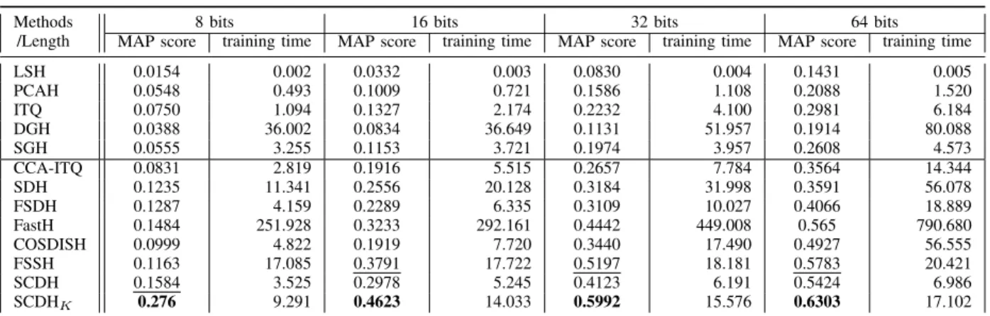
Table VIII: The MAP scores and training time costs (in seconds) of different hashing methods, for unseen classes. (a) Caltech256{Train:Test =70%classes :30%classes}

Methods /Length

LSH 0.0154 0.002 0.0332 0.003 0.0830 0.004 0.1431 0.005 PCAH 0.0548 0.493 0.1009 0.721 0.1586 1.108 0.2088 1.520 ITQ 0.0750 1.094 0.1327 2.174 0.2232 4.100 0.2981 6.184 DGH 0.0388 36.002 0.0834 36.649 0.1131 51.957 0.1914 80.088 SGH 0.0555 3.255 0.1153 3.721 0.1974 3.957 0.2608 4.573 CCA-ITQ 0.0831 2.819 0.1916 5.515 0.2657 7.784 0.3564 14.344 SDH 0.1235 11.341 0.2556 20.128 0.3184 31.998 0.3591 56.078 FSDH 0.1287 4.159 0.2289 6.335 0.3109 10.027 0.4066 18.889 FastH 0.1484 251.928 0.3233 292.161 0.4442 449.008 0.565 790.680 COSDISH 0.0999 4.822 0.1919 7.720 0.3440 17.490 0.4927 56.555 FSSH 0.1163 17.085 0.3791 17.722 0.5197 18.181 0.5783 20.421 SCDH 0.1584 3.525 0.2978 5.245 0.4123 6.191 0.5424 6.986 SCDHK 0.276 9.291 0.4623 14.033 0.5992 15.576 0.6303 17.102

(b) Cifar10{Train:Test =70%classes :30%classes}

Methods /Length

LSH 0.0871 0.001 0.0971 0.001 0.1160 0.001 0.1222 0.002 PCAH 0.0958 0.258 0.0926 0.261 0.1034 0.313 0.1066 0.482 ITQ 0.1100 0.853 0.1291 1.346 0.1400 3.574 0.1445 6.277 DGH 0.0916 71.532 0.0893 78.963 0.0945 88.605 0.1016 114.303 SGH 0.1099 1.652 0.1059 2.036 0.1142 3.023 0.1156 6.542 CCA-ITQ 0.1607 1.718 0.1653 3.489 0.2188 5.215 0.2197 8.989 SDH 0.2002 6.833 0.2045 15.385 0.2608 19.804 0.2849 33.855 FSDH 0.1781 3.156 0.2292 4.995 0.2776 6.180 0.2778 7.443 HC-SDH n/a n/a 0.4205 3.229 0.4270 3.765 0.4295 3.803 FastH 0.3237 378.261 0.4324 541.176 0.5067 812.296 0.5149 1662.214 COSDISH 0.2288 5.119 0.2756 7.867 0.3607 22.784 0.3846 99.903 FSSH 0.4331 63.881 0.4861 67.397 0.5308 70.957 0.5597 74.212 SCDH 0.3730 3.091 0.3992 4.138 0.4984 6.187 0.5108 7.020 SCDHK 0.4450 7.704 0.5126 8.270 0.5609 10.314 0.5807 11.950

(c) NUS-WIDE{Train:Test =70%concepts :30%concepts}

Methods /Length

LSH 0.2039 0.156 0.2081 0.559 0.2176 0.753 0.2176 0.771 PCAH 0.2412 0.890 0.2572 1.703 0.2588 2.049 0.2613 2.558 ITQ 0.2576 3.057 0.2580 7.021 0.2638 12.098 0.2647 17.291 DGH 0.2068 398.513 0.2148 505.936 0.2155 799.486 0.2187 916.381 SGH 0.2147 8.891 0.2223 12.411 0.2274 39.229 0.2344 143.068 CCA-ITQ 0.3048 6.464 0.3380 8.001 0.3448 17.176 0.3691 27.981 SDH 0.2859 25.959 0.3204 35.711 0.3302 58.444 0.3399 138.303 FSDH 0.3144 7.464 0.3257 11.685 0.3352 27.895 0.3605 44.902 FastH — — — — — — — — COSDISH 0.3662 11.422 0.3777 25.042 0.3829 90.281 0.3914 282.240 FSSH 0.4100 675.187 0.4268 685.416 0.4302 696.424 0.4381 718.315 SCDH 0.4136 6.219 0.4247 11.408 0.4354 26.034 0.4397 59.489 SCDHK 0.4326 37.024 0.4380 45.143 0.4515 58.865 0.4587 105.689

search strategies, i.e., “+BF”, “+HI”, “+GH” and “+PQ”16_{. The}

results on Cifar10 and NUS-WIDE are reported in TableVII, where the effectiveness is measured by the precision of the top-1000 search results (P@1000) on the test set, and the efficiency is measured by the retrieval time (in seconds). It can be seen that the standard binary SCDHK reaches similarly high

P@1000 scores as the thorough brute-force search strategy, but only with a fraction of the retrieval time. Moreover, by 16_{For “+HI” and “+GH”, the number of clusters and the number of} candidates are set to 10 and 2000 respectively. For “+PQ”, the CPU version of the faiss [58] implementation is employed, for a fair comparison.

enforcing the binary constraint and directly optimizing the binary codes to represent the data, SCDHK outperforms the

real-valued model using any of the other three search strategies.

K. Unseen Classes

The experimental results in TableII are obtained under the traditional configuration where each class has some examples for training and some examples for testing, as in most learning to hash papers [14], [18], [17], [52], [26], [24], [45], [44]. However, a new evaluation protocol “retrieval of unseen classes” [53] has recently been proposed to measure the

(15)

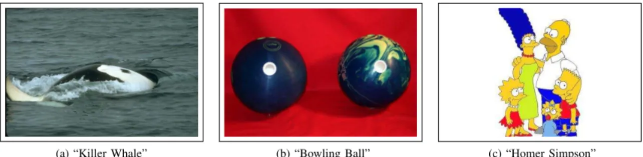
(a) “Killer Whale” (b) “Bowling Ball” (c) “Homer Simpson”

Figure 5: The three randomly selected queries for our image retrieval case study. Their top-20 search results on Caltech256 are shown in Figs. 6 ,7and8 respectively.

SCDHK: 20/20 SCDH: 20/20 COSDISH: 13/20 SDH: 18/20 FastH: 10/20 LSH: 5/20 PCAH: 6/20 ITQ: 14/20 DGH: 0/20 SGH: 4/20 FSSH: 20/20

Figure 6: Retrieval results: “Killer Whale” (the bounding boxes are green for correct results and red for wrong ones).

generalization ability of the learned hash functions on unseen classes (i.e., the classes not appeared in the training stage at all).

Following the configuration in [53], [54], we randomly select about 70% of the classes and use their examples to learn the hash functions, while the examples in the rest 30% classes are reserved for the purpose of evaluation only. Specifically, on Caltech256, we have 180 classes for training and the other 76 classes for testing; on Cifar10, we have 7 classes for training and the other 3 classes for testing; on the multi-labeled dataset NUS-WIDE, the examples labeled by at least one of the selected 7 classes are used for training and the remaining examples are used for testing. Under the same settings as described before in Section VI-C, we conduct experiments on the retrieval of unseen classes and report the results in TableVIII. Similar to the previous experimental results, SCDH/SCDHK demonstrates

not only higher effectiveness (in terms of MAP scores) than all the other hashing methods in comparison but also higher efficiency (in terms of training speeds) than the supervised ones among them.

L. Case Study

Here we examine the top-20 image retrieval results for three randomly selected queries — “Killer Whale” (Fig.5a), “Bowling Ball” (Fig. 5b) and “Homer Simpson” (Fig. 5c) —-on Caltech256 (as described in Secti—-onVI-A), using different hashing methods under our investigation, with the code length set to 32 bits.

In Figs. 6 , 7and 8, the first six rows correspond to six supervised methods while the remaining five rows correspond to five unsupervised methods. Overall, the supervised methods perform far better than the unsupervised methods. In particular, our proposed method SCDHK could achieve 100% accuracy

(20/20) for every given query, significantly outperforming other methods such as COSDISH, SDH and FastH. Furthermore, the performances of SCDH/SCDHK are more stable than those of

the other methods across different queries.

Specifically, in Fig. 6, both SCDH and SCDHK could

recognize “Killer Whale” perfectly under different color backgrounds while the other methods would make some mistakes. For example, the competitive method COSDISH

(16)

6CD+. 6CD+ &26',6+ 6'+ )DVW+ /6+ 3&$+ ,74 '*+ 6*+ )SS+

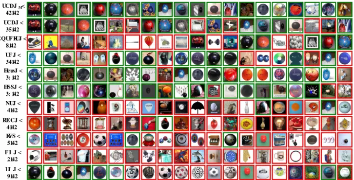
Figure 7: Retrieval results: “Bowling Ball” (the bounding boxes are green for correct results and red for wrong ones).

SCDHK: 20/20 SCDH: 20/20 COSDISH: 0/20 SDH: 19/20 FastH: 20/20 LSH: 3/20 PCAH: 9/20 ITQ: 3/20 DGH: 0/20 SGH: 6/20 FSSH: 20/20

Figure 8: Retrieval results: “Homer Simpson” (the bounding boxes are green for correct results and red for wrong ones).

often confuses tires with killer whales; FastH and SGH often incorrectly returns swans that are similar to killer whales from the appearance. In Fig. 7, SCDHK successfully tells

the difference between “Bowling Ball” and other ball-like objects, but the other methods including COSDISH, ITQ, and SGH often fail to distinguish them and thus perform badly. In Fig. 8, SCDH/SCDHK again could reach 100% accuracy,

but COSDISH would collapse: it could not find any image of “Homer Simpson” at all.

It is worth mentioning that FSSH, probably the strongest

baseline method, also performs well for the three given queries. Nevertheless, FSSH is still slightly inferior to SCDHK in the

case of “Bowling Ball” (Fig.7), which reflects the outstanding ability of our proposed methods.

In summary, these three concrete queries have intuitively illustrated the substantial performance improvements that SCDH/SCDHK could make on existing methods for

(17)

VII. CONCLUSION

In this paper, we improve supervised discrete hashing by maintaining two strong constraints (balance and decorrelation of hash bits) and propose a fast optimization algorithm for it. Although such constraints are known to be beneficial for hashing in previous studies, to our knowledge this is the first time that the hard discrete optimization problem with all those constraints is shown to have efficient solutions. The developed algorithm SCDH, and its kernelized variant SCDHK, can learn

the binary codes and the hash function from labelled data simultaneously. They have been demonstrated to outperform state-of-the-art supervised learning to hash methods for large-scale image retrieval in terms of both MAP scores and training speeds.

ACKNOWLEDGMENT

Thanks to the support of China Scholarship Council (CSC), Yong has been funded as a visiting PhD student at Birkbeck and UCL from 01/2018 to 01/2019. This work is also supported in part by China Postdoctoral Science Foundation.

REFERENCES

[1] Ruslan Salakhutdinov and Geoffrey E. Hinton,Semantic Hashing. In Int. J. Approx. Reasoning, 969–978, 2009.1

[2] Aristides Gionis, Piotr Indyk and Rajeev Motwani,Similarity Search in High Dimensions via Hashing. In VLDB, 518–529, 1999. 1,6

[3] Yunchao Gong, Svetlana Lazebnik, Albert Gordo and Florent Perronnin, Iterative Quantization: A Procrustean Approach to Learning Binary Codes for Large-Scale Image Retrieval. In IEEE Trans. on Pattern Anal. Mach. Intell., 2916–2929, 2013. 1,6

[4] Xi Li, Guosheng Lin, Chunhua Shen, Anton van den Hengel and Anthony R. Dick,Learning Hash Functions Using Column Generation. In ICML, 142–150, 2013.

[5] Jingkuan Song, Yang Yang, Yi Yang, Zi Huang and Heng Tao Shen, Inter-media Hashing for Large-Scale Retrieval from Heterogeneous Data Sources. In SIGMOD, 785–796, 2013. 1

[6] Kilian Q. Weinberger, Anirban Dasgupta, John Langford, Alexander J. Smola and Josh Attenberg,Feature Hashing for Large Scale Multitask Learning. In ICML, 1113–1120, 2009. 1

[7] Konstantin Berlin, Sergey Koren, Chen-Shan Chin, James P. Drake, Jane M. Landolin and Adam M. Phillippy,Assembling Large Genomes with Single-Molecule Sequencing and Locality-Sensitive Hashing. In Nature Biotechnology, 623–630, 2015.1

[8] Baris Coskun, Bulent Sankur and Nasir D. Memon, Spatio-Temporal Transform Based Video Hashing. In IEEE Trans. on Multimedia, 1190– 1208, 2006.1

[9] Yair Weiss, Antonio Torralba and Robert Fergus,Spectral Hashing. In NIPS, 1753–1760, 2008.1,2,3,6

[10] Wei Liu, Jun Wang, Sanjiv Kumar and Shih-Fu Chang,Hashing with Graphs. In ICML, 1–8, 2011. 1,2

[11] Wei Liu, Cun Mu, Sanjiv Kumar and Shih-Fu Chang,Discrete Graph Hashing. In NIPS, 3419–3427, 2014.1,3,5,6

[12] Qing-Yuan Jiang and Wu-Jun Li,Scalable Graph Hashing with Feature Transformation. In IJCAI, 2248–2254, 2015. 1,6,9

[13] Dell Zhang, Jun Wang, Deng Cai and Jinsong Lu,Self-Taught Hashing for Fast Similarity Search. In SIGIR, 18–25, 2010. 1,2,3

[14] Jun Wang, Ondrej Kumar and Shih-Fu Chang,Semi-Supervised Hashing for Scalable Image Retrieval. In CVPR, 3424–3431, 2010. 1,2,12

[15] Mohammad Norouzi and David J. Fleet, Minimal Loss Hashing for Compact Binary Codes. In ICML, 353–360, 2011. 1

[16] Wei Liu, Jun Wang, Rongrong Ji, Yu-Gang Jiang and Shih-Fu Chang, Supervised Hashing with Kernels. In CVPR, 2074–2081, 2012.1,2,4,

6,9

[17] Fumin Shen, Chunhua Shen, Wei Liu and Heng Tao Shen,Supervised Discrete Hashing. In CVPR, 37–45, 2015.2,6,12

[18] Guosheng Lin, Chunhua Shen, Qinfeng Shi, Anton van den Hengel and David Suter,Fast Supervised Hashing with Decision Trees for High-Dimensional Data. In CVPR, 1971–1978, 2014.1,4,6,12

[19] Tiezheng Ge, Kaiming He and Jian Sun,Graph Cuts for Supervised Binary Coding. In ECCV, 250–264, 2014.1

[20] Guosheng Lin, Chunhua Shen, David Suter and Anton van den Hengel, A General Two-Step Approach to Learning-Based Hashing. In ICCV, 2552–2559, 2013. 1

[21] Wu-Jun Li, Sheng Wang and Wang-Cheng Kang,Feature Learning Based Deep Supervised Hashing with Pairwise Labels. In IJCAI, 1711–1717, 2016. 1,2,10

[22] Guiguang Ding, Yuchen Guo and Jile Zhou,Collective Matrix Factor-ization Hashing for Multimodal Data. In CVPR, 2083–2090, 2014.

1

[23] Gou Koutaki, Keiichiro Shirai and Mitsuru Ambai,Hadamard Coding for Supervised Discrete Hashing. In IEEE Trans. Image Processing, 5378–5392, 2018. 6,7

[24] Sen Su, Gang Chen, Xiang Cheng and Rong Bi,Deep Supervised Hashing with Nonlinear Projections. In IJCAI, 2786–2792, 2017. 1,6,12

[25] Qing-Yuan Jiang and Wu-Jun Li,Asymmetric Deep Supervised Hashing. In AAAI, 3342–3349, 2018. 1

[26] Wang-Cheng Kang, Wu-Jun Li and Zhi-Hua Zhou,Column Sampling Based Discrete Supervised Hashing. In AAAI, 1230–1236, 2016. 2,3,

6,12

[27] Griffin Gregory, Holub Alex and Perona Pietro, Caltech-256 Object Category Dataset. In California Institute of Technology, 2007. 6

[28] Alex Krizhevsky,Learning Multiple Layers of Features from Tiny Images. In Master’s thesis, Department of Computer Science, University of Toronto, 2009. 6

[29] Alex Krizhevsky, Ilya Sutskever and Geoffrey E. Hinton,ImageNet Classification with Deep Convolutional Neural Networks. In NIPS, 1106–1114, 2012.

[30] Peichao Zhang, Wei Zhang, Wu-Jun Li and Minyi Guo,Supervised Hashing with Latent Factor Models. In SIGIR, 173–182, 2014. 6

[31] Yunchao Gong and Svetlana Lazebnik,Iterative Quantization: A Pro-crustean Approach to Learning Binary Codes. In CVPR, 817–824, 2011.

6

[32] Zhongming Jin, Yao Hu, Yue Lin, Debing Zhang, Shiding Lin, Deng Cai and Xuelong Li,Complementary Projection Hashing. In ICCV, 257–264, 2013. 6

[33] Jia Deng, Wei Dong, Richard Socher, Li-Jia Li, Kai Li and Fei-Fei Li,ImageNet: A Large-Scale Hierarchical Image Database. In CVPR, 248–255, 2009.

[34] Ruimao Zhang, Liang Lin, Rui Zhang, Wangmeng Zuo and Lei Zhang, Bit-Scalable Deep Hashing With Regularized Similarity Learning for Image Retrieval and Person Re-Identification. In IEEE Trans. on Image Processing, 4766–4779, 2015. 1

[35] Brian Kulis and Kristen Grauman,Kernelized Locality-Sensitive Hashing for Scalable Image Search. In ICCV, 2130–2137, 2009. 4

[36] Ke Jiang, Qichao Que and Brian Kulis,Revisiting Kernelized Locality-Sensitive Hashing for Improved Large-Scale Image Retrieval. In CVPR, 4933–4941, 2015.4

[37] Tat-Seng Chua, Jinhui Tang, Richang Hong, Haojie Li, Zhiping Luo and Yantao Zheng,NUS-WIDE: A Real-World Web Image Database from National University of Singapore. In CIVR, 2009.6

[38] Zijia Lin, Guiguang Ding, Mingqing Hu and Jianmin Wang, Semantics-Preserving Hashing for Cross-View Retrieval. In CVPR, 3864–3872, 2015. 6

[39] Dongqing Zhang and Wu-Jun Li,Large-Scale Supervised Multimodal Hashing with Semantic Correlation Maximization. In AAAI, 2177–2183, 2014. 3

[40] Ning Li, Chao Li, Cheng Deng, Xianglong Liu and Xinbo Gao,Deep Joint Semantic-Embedding Hashing. In IJCAI, 2397–2403, 2018.2

[41] Weiming Hu, Yabo Fan, Junliang Xing, Liang Sun, Zhaoquan Cai and Stephen J. Maybank,Deep Constrained Siamese Hash Coding Network and Load-Balanced Locality-Sensitive Hashing for Near Duplicate Image Detection. In IEEE Trans. on Image Processing, 4452–4464, 2018. 2

[42] Fumin Shen, Xin Gao, Li Liu, Yang Yang and Heng Tao Shen,Deep Asymmetric Pairwise Hashing. In ACM Multimedia, 1522–1530, 2017.

2

[43] Haomiao Liu, Ruiping Wang, Shiguang Shan and Xilin Chen,Deep Supervised Hashing for Fast Image Retrieval. In CVPR, 2064–2072, 2016. 2

[44] Xin Luo, Liqiang Nie, Xiangnan He, Ye Wu, Zhen-Duo Chen and Xin-Shun Xu,Fast Scalable Supervised Hashing. In SIGIR, 735–744, 2018.

2,6,9,12

[45] Jie Gui, Tongliang Liu, Zhenan Sun, Dacheng Tao and Tieniu Tan,Fast Supervised Discrete Hashing. In IEEE Trans. on Pattern Anal. Mach. Intell., 490–496, 2018. 2,6,9,12