Board of Directors Educational Diversity and Acquirer’s
Announcement Cumulative Abnormal Returns
Daniel Rau
A Thesis in the John Molson School of Business
Presented in Partial Fulfillment of the Requirements for the
Degree of Master of Science in Administration (Finance) at
Concordia University
Montreal, Quebec, Canada
May 2016
CONCORDIA UNIVERSITY
School of Graduate Studies
This is to certify that the thesis prepared
By:
Daniel Rau
Entitled:
Board of Directors Educational Diversity and Acquirer’s
Announcement Cumulative Abnormal Returns
and submitted in partial fulfillment of the requirements for the degree of
Master in Administration (Finance)
complies with the regulations of the University and meets the accepted
standards with respect to originality and quality.
Signed by the final examining committee:
Dr. Mahesh Sharma___________________
Chair
Dr. Ravi Mateti_______________________
Examiner
Dr. Saif Ullah_________________________
Examiner
Dr. Sandra Betton_____________________
Supervisor
Approved by
Dr. Thomas Walker___________________
Graduate Program Director
Dr. Stephane Brutus___________________
Dean of Faculty
iii
Abstract
Board of Directors Educational Diversity and Acquirer’s Announcement Cumulative
Abnormal Returns
Daniel Rau
The aim of this paper is to study the relationship between the educational diversity of the board
directors and the acquirer’s cumulative abnormal return associated with the announcement of a
M&A. The results show that the cumulative abnormal return is positively related to educational
diversity, however the model exhibits significant heteroscedasticity and therefore the results
cannot be accepted as conclusive. Several attempts at fixing the heteroscedasticity failed and
statistically appropriate model relating the cumulative abnormal returns to the explanatory
variables is yet to be found.
iv
Acknowledgements
I am very thankful to my supervisor Prof. Betton for her invaluable comments and guidance
throughout the elaboration of this thesis. I am also very thankful to all the Professors who taught
me for making my MSc studies such a great learning experience, and my family and friends for
supporting and encouraging me.
v
Table of Contents
1. Introduction……….……….………...1
2. Literature Review….………..1
3. Hypothesis……….……12
4.
Methodology……….……….…12
5. Summary Statistics……….………...15
6. Results……….. ………….………..……..18
7. Box Cox Transformation………...25
8. Feasible Generalized Least Squares……….………..27
9. Flexible Functional Form……….……….28
10. Omitted variable bias….. ………31
11. Heteroscedasticity consistent standard errors………..………32
12. Conclusion………...…34
13. Further Research………..34
14. References………....35
vi
List of Tables
Table1. Multiple Intelligences and Occupations……….……5
Table2. Literature review summary………..……….………11
Table3. Percentage of the Education Categories………..……….15
Table4. Percentage of Females………..15
Table5. Percentage of Females by Educational Category…….………….…….………..16
Table6. Independent Variable Description……….….……….……….19
Table7. Regression results……….……….……….………..20
Table8. Heteroscedasticity Tests………. …….……….………...22
Table9. Normality of the errors test………. …….………..………..30
Table10. Regression with HCSE………...33
List of Figures
Figure1. Cumulative Abnormal Return Distribution ………….……….………..17
Figure2. Heteroscedasticity depiction………...……….………21
Figure3. Residual vs CAR3………...……….………...23
Figure4. Box Cox transformation illustration……….………...26
Figure5. First nonlinear model………...……….………...30
1 Introduction
Through acquisitions firm-specific assets housed within one organization are merged with assets in another organization to improve the productivity of the combined assets (Anand and Singh, 1997). The market reacts to the news of the acquisition by influencing the stock prices around the announcement time of the parties involved reflecting the market’s expectation about the profitability of this acquisition. The event study methodology is based on the fundamental idea that stock prices represent the discounted expected value of firms’ future stream of profits and is useful in order to understand the relationship between different firm characteristics and the event’s impact on the market’s reaction as reflected in the abnormal returns at the announcement.
The impact of the announcement on the target is primarily determined by the premium paid and empirical studies, such as Franks et al. (1991), Dodd et al. (1977) and Jensen et al. (1983), generally conclude that targets earn a significant abnormal return while, on average, the bidding firms earn insignificantly different from zero returns. In order to study the quality of the acquisition from a value creating decision point of view I focus on the acquirers because the acquirers pay to acquire a target in order to get a benefit from that target. The determinants of performance of acquiring firms have been extensively studied empirically and in this study I use, as control variables, many of these previously examined determinants. The focus of this study is the acquirer’s board of directors because it is the ultimate decision maker in M&As, and in this study I rely upon two streams of research: the role of education and the role of diversity in firm performance. In this paper, I examine the impact of board educational diversity on the acquirer’s cumulative abnormal return around the date of an acquisition in order to indirectly assess the role of educational diversity on the quality of decision making by boards of directors.
Literature Review Educational diversity
As educational diversity is the primary focus of this study, I will begin by surveying the primary research in the area of manager education before moving on to the more general area of diversity.
According to Becker (1993), human capital encompasses the knowledge, information, ideas, skills, and health of individuals, and age and education are a proxy for human capital. Education increases the value of human capital; thus, it may be an important characteristic for board members. Daily et al. (1994) use
2 education to represent the quality of a firm’s board and its decision making ability. Top managers of the firm are hired because of their superior ability and according to Bhagat et al. (2010), such ability consists of observable characteristics (e.g. educational backgrounds and work experiences) and unobservable characteristics (e.g. leadership and entrepreneurial skills). They contend that since the unobservable characteristics are relatively difficult to identify and measure, the observable characteristics may play an important role in determining this superior ability. Hambrick and Mason (1984) also state that observable characteristics (education and experience) are considered valid proxies for cognitive orientation, values, and knowledge base, which may in turn significantly influence decision making and managerial behavior. Gottesman and Morey (2006) state that educational qualification may be a proxy for intelligence and more intelligent managers are expected to be better decision makers than their less intelligent peers. Bantel and Jackson (1989) and Wiersema and Bantel (1992) suggest that CEOs with higher educational attainments are better able to process information and accept significant changes within the firm. Martins et al. (1996) and Williams et al. (1998) argue that board members with different functional, industrial, and educational backgrounds are more likely to experience differences in the way that they perceive, process, and respond to issues with which they are confronted and these differences are likely to influence positively the level of cognitive conflict. Cognitive conflict is the mental discomfort that people experience when confronted with new information that contradicts their prior beliefs and ideas, pushing them either to assimilate the new information into an existing schema or to accommodate the new information by creating a new schema. Jackson (1992) finds that individuals with dissimilar backgrounds are likely to possess different knowledge, skills, and expertise, which, when brought to a team decision-making process, will increase its quality. Jehn et al. (1997) found that differences in educational background lead to an increase in task related debates in work teams.
Addressing the association between the demographic diversity of top managers and firm performance, Smith et al. (1994) find that educational heterogeneity positively influences return on investments (ROI). Using growth in market share and growth in profits as dependent variables, Hambrick et al. (1996) provide evidence that the relationship between the average education level of top management team members and firm performance is positive and significant. Anderson et al. (2011) show that even though managers prefer homogenous boards, shareholders value diversity in terms of educational background and that there is a positive relationship between board heterogeneity and firm performance. But diversity might also pose problems, namely the difficulty of integration. Westphal and Milton (2000) find that homogeneity with respect to educational affiliation enhances social integration on boards. Burgess et al. (2000) found that social similarity (such as education and demography) may be an important factor for appointments to the board because individuals will often have shared values and attitudes and derive
self-3 esteem from group membership. Similarity leads to self-validation, ease of communication and trusting relationships. The preference for those that are perceived as similar is particularly prevalent in situations of uncertainty and unfamiliarity. But the realization of the benefits that diversity can bring pushes firms to embrace diversity and Singh et al. (2011) in their study report of an increasing trend among companies to hire business executives from a variety of streams, especially from the broad stream of humanities and social sciences, and not just the stream of management and business studies.
Research was also conducted for specific types of education. With respect to the firm’s research and development (R&D) spending, a number of studies provide evidence that CEOs with degrees in technical fields are likely to allocate more resources for the funding of R&D activities (Finkelstein and Hambrick, 1996; Barker and Mueller, 2002). Graham and Harvey (2002) suggest that chief financial officers (CFOs) holding MBA degrees are more likely to follow academic advice and employ present value techniques in evaluating new projects. Guner et al. (2008) find that directors from a corporate banking background are associated with poor acquisition outcomes, although it is unclear if this is a specific experience or a habitual way of thinking which is at fault. Wadhwa et al. (2008) surveyed 652 US born entrepreneurs who started tech and engineering companies and found that 92% held bachelor’s degrees, 31% held master’s degrees and 10% held PhDs. Nearly half of these degrees were in Science, Technology, Engineering and Mathematics (STEM). One third of the degrees were business, accounting and finance. Founders holding MBA degrees established companies more quickly than others.
There is a considerable difference between academic and professional opinions regarding the importance of skills. Shuayto (2013) conducted a survey research asking a group of prospective employers and a group of business school deans/directors of MBA programs to rank the most and least important skills for MBA graduates. According to the prospective employer respondents, the most important skills to be obtained by graduates are (in order of importance) responsibility and accountability, interpersonal skills, oral communication, teamwork, ethical values, decision-making and analytical skills, and creativity and critical thinking. Those attributes believed to be less important included written communication, time and project management, persuasive ability, presentation skills, ability to assimilate new technologies, computer skills, and global awareness. According to the business school deans/directors of MBA programs, the most important skills are (in order of importance) oral communication, written communication, interpersonal skills, decision making and analytical ability, responsibility and
accountability, ability to work in teams, creativity and critical thinking skills. Deans/directors indicated that ethical values, computer skills, time and project management, persuasive ability and global awareness were less important attributes. Although Shuayto (2013) isn’t specifically about board directors, it is
4 interesting because it studies the skills needed for MBA graduates who are expected to be future
managers. Given the difference of opinion I do not try to rank skills and education degrees by degree of importance but rather study the impact of their diversity on the board’s M&A decisions.
I also look at graduate and postgraduate educational degrees. Audretsch and Lehmann (2006) argue that an academic degree such as a PhD could signal the superior quality of the human capital of the board members. Such a degree could indicate the director having spent a substantial time in the academic environment, which could have provided the director with valuable knowledge necessary for strategic decision making (Carpenter and Westphal, 2001). In accordance with this view, Dalziel et al. (2011) argue that advanced degrees such as PhD could equip directors with extra skills that could be beneficial for the firm, especially in their R&D efforts. Ruigrok et al., (2006) find that a higher percentage of directors with PhDs are appointed to the boards as independent directors, who are expected to be more effective monitors, which is also a trait expected from directors with high levels of education.
In this paper I will use educational degrees as proxies for specific types of intelligence based on Gardner’s multiple intelligence theory. The theory of multiple intelligences was proposed in 1983 by American developmental psychologist Howard Gardner in his book Frames of Mind: The Theory of Multiple Intelligences and this theory differentiates intelligence into specific abilities rather than seeing intelligence as dominated by a single general ability. Gardner articulated eight criteria for a behaviour to be considered an intelligence: potential for brain isolation by brain damage, place in evolutionary history, presence in core operations, susceptibility to encoding (symbolic expression), a distinct developmental progression, the existence of savants, prodigies and other exceptional people, and support from
experimental psychology and psychometric findings. Based on these criteria Gardner identifies the following abilities as an intelligence type: musical-rhythmic, visual-spatial, verbal-linguistic, logical-mathematical, bodily-kinesthetic, interpersonal, and intrapersonal. Gardner argues that the IQ tests focus mostly on logical and linguistic intelligence and therefore misrepresent other abilities or simply do not capture them at all.
Based on this theory Sharifi (2006) administered the Multiple Intelligence Questionnaire adapted from Douglas and Harms to 120 secondary school students and found a low to moderate but significant correlation among different kinds of intelligence and related school subject scores. He also found that interpersonal and intrapersonal intelligence scores account for 22% of the variance, illustrating the difficulty in measuring these types of intelligences. Mankad (2015) in his paper presented an expert system that classifies an individual’s abilities, by conducting the Multiple Intelligences Questionnaire, into one of the three fields: engineering, management and science, thus relating the Multiple Intelligences Theory with specific fields.
5 The association between a primary intelligence and occupation was described in Dr. Thomas Armstrong book Multiple Intelligences in the Classroom (1994) and a short list is presented in table 1 below.
Table 1
Multiple Intelligences and Occupations
Linguistic Intelligence librarian, curator, speech pathologist, writer, radio or TV announcer, journalist, lawyer
Logical-Mathematical Intelligence auditor, accountant, mathematician, scientist, statistician, computer analyst, technician
Spatial Intelligence engineer, surveyor, architect, urban planner, graphic artist, interior decorator, photographer, pilot
Bodily-Kinesthetic Intelligence physical therapist, dancer, actor, mechanic, carpenter, forest ranger, jeweler
Musical Intelligence musician, piano tuner, music therapist, choral director, conductor
Interpersonal Intelligence administrator, manager, personnel worker, psychologist, nurse, public relations person, social director, teacher
Intrapersonal Intelligence psychologist, therapist, counselor, theologian, program planner, entrepreneur
The directors’ education is a new and growing field of study and there are several working papers
specifically studying it. Wagner et al. (2015) find that more qualified directors receive higher pay, largely because they are allocated more board functions relative to CEO-appointed (“co-opted”) directors, and announcement returns around unexpected director departures suggest that the market values qualified directors and discounts co-opted ones. Dionne et al. (2013) find a difference between the impact of limited experience and education-enhanced experience by showing that financially educated directors encourage the use of derivatives and hedging activity in contrast to directors with only financial or accounting experience or accounting. Kalyta (2014) shows that director education, especially in science and engineering, positively affects ROE for technology companies.
The other control variables include variables that were already used in previous papers studying the acquirer’s abnormal return around announcement date, as well as variables that were not used in that kind of research, but were found to be important board attributes. It is important to include control variables because they might have an influence on the cumulative abnormal return and omitting them can result in omitted variable bias which I will mention later in the paper.
6 Board size
Ning et al. (2010) find that most boards have between eight and eleven directors. Boards with seven or fewer directors tend to increase their size, while large boards with twelve or more directors tend to reduce their size to the target zone. Lipton and Lorsch (1992) and Jensen (1993) argue that large boards can be costly. Larger boards increase operational complexity and increase the potential for dissention among members. When board size increases, agency problems in the boardroom increase simultaneously, leading to more free-riding problems and internal conflicts among directors. On the other hand, Dalton et al. (1999) find a non-zero and positive board size and performance association. Booth and Deli (1996) argue that environmental uncertainty generally leads to large board size.
Multiple directorships
There are two competing hypotheses on the issue. First, the number of outside directorships may signal director quality (Fama and Jensen, 1983). Mace (1996) suggests that outside directorships are perceived to be valuable because they provide executives with prestige, visibility, and commercial contacts.
Directors with more outside board seats may be more experienced, provide better advice, and offer better monitoring. If this is the case, they should help attenuate agency costs and discourage value-reducing acquisitions that are motivated by agency conflicts. This hypothesis is called the reputation hypothesis and predicts that market reaction is more positive (or less negative) for acquiring firms where directors hold more outside board seats. By contrast, the busyness hypothesis contends that directors with too many outside board seats may be so busy that they do not function as effective monitors. This diminished oversight may lead to more severe agency conflicts, because managers are better able to pursue their own private benefits at the expense of the shareholders. One well-known consequence of agency conflicts is the depletion of free cash flows on unnecessary acquisitions that destroy value (Jensen, 1986).
Brown and Maloney (1999) compare the board characteristics of acquiring firms that are well and poorly governed, respectively, and investigate the role of directors in acquisition decisions. They find that directors in bad acquirers hold more directorships (2.35 on average) compared to those in good acquirers (1.87 on average). Ahn et al. (2010) show that the effect of multiple directorships is nonlinear on
acquisition performance. Multiple outside board seats induce negative announcement returns only when the number of multiple directorships reaches a high threshold. In the same logic Core et al. (1999) found that too many directorships may lower the effectiveness of outside directors as corporate monitors. Fich and Shivdasani (2006) find that firms with boards where the majority of outside directors are busy (i.e., holding three or more directorships) are associated with weak corporate governance, lower market to-book ratios, weaker profitability, and lower sensitivity of CEO turnover to firm performance.
7 CEO tenure
According to the upper-echelons perspective (Hambrick & Mason, 1984), CEOs act based on their understanding of the strategic situations they confront. This understanding is significantly shaped by their tenure (Souder, Simsek & Johnson, 2012), which mirrors their paradigms, skills, knowledge and
cognition (Barker & Mueller, 2002) acquired during their tenure.
Henderson et al. (2006) view tenure effect as being nonlinear and argue that CEOs pass through two phases during their time in office: the first phase is an initial period of adaptive improvement, and in the second phase, CEOs become overly committed to existing approaches and tend to embrace the status quo, so the effectiveness of CEOs increases up to a certain point in time and then starts diminishing.
This nonlinear relation was seen in the influence of CEO tenure on firm inventiveness (Wu, Levitas & Priem, 2005) and firm internationalization (Jaw & Lin, 2009) and is likely to follow the pattern of an inverted-U shape.
Walters et al. (2007) explore the impact of CEO tenure on returns to shareholders arising from acquisition announcements. Further, they consider the value added for shareholders when the board of directors is composed in such a way as to enhance vigilance. In the absence of a vigilant board, CEO tenure is
positively associated with performance at low to moderate levels of tenure, and negatively associated with performance when tenure further rises to substantial levels. In the presence of a vigilant board, however, shareholder interests can be advanced even at high levels of CEO tenure.
Industry Relatedness
The ability to use new information to solve problems is enhanced when the new knowledge is related to what is already known (Cohen and Levinthal, 1990).Acquiring unrelated businesses reduces productivity and is found to be problematic (Singh and Montgomery, 1987) so I will look at whether the bidder and the target are from the same industries using the 2 and 3 digit SIC codes.
Female directors
Research suggests that women exhibit less overconfidence compared to men (Johnson et al., 2006), with overconfidence linked to the propensity to take excess risks and make poor financial decisions (Barber and Odean, 2001). Thus a greater representation of women should reduce excessively risky decisions and it was found that an increased female director representation has been linked to higher-quality earnings (Srinidhi et al. 2011). Carter et al. (2003) find that ethnic and gender diversity among a board of directors
8 is associated with higher firm value for a sample of large US firms which implies that there are gender and ethnic specific characteristics which contribute to value creation and better decision making. Levi et al. (2013) found an inverse relation between the number of bids and premium paid, and the number of females on the board and this again reflects women’s greater aversion to risk and overspending. So a greater female representation can be viewed as a contribution to monitoring and risk reduction. Firm size
Netter et. al (2011) find acquisitions to generally be value-neutral for large companies, in addition to being a distraction of management focus. Swanstorm (2006) find a significant negative relationship between the log of firm size and M&A CAR, and a positive relationship with a dummy variable
corresponding to cash acquisition. Stulz et al.(2004) find that the announcement return for acquiring-firm shareholders is roughly two percentage points higher for small acquirers irrespective of the form of financing and whether the acquired firm is public or private. However, Alexandridis, et al. (2013) show that larger bidders make better takeovers. It should be noted that Stulz et al. sample is dominated by nonpublic targets while Alexandridis et al.(2013) exclusively work on a subsample of public targets. In my case I have both public and public targets (which will be discussed later) and therefore the size effect will be viewed globally irrespective of firm type.
Intense Monitoring
Agency theorists argue that independent directors are charged with the responsibility of monitoring managers to act in the best interests of shareholders (Jensen & Meckling, 1976)and of facilitating access to critical information and valuable resources (Chen, 2011).
Kroll et al. (1990) found that CEO compensation increased following acquisitions due in part to the increased size of the firm, so managers may behave in their own interest in M&A decisions as opposed to shareholders’ interest. McWilliams and Sen (1997) observe negative market reaction to antitakeover announcements. This reaction is more pronounced when the board is dominated by insider and gray directors and where the CEO is also the chairman of the board. Faleye et al. (2011) show that boards where the majority of independent board members qualify as “intense monitors” (the members serve on at least two of the three principal monitoring committees – audit, compensation and nominating) display superior monitoring performance ,although too much board monitoring can decrease shareholder value (Almazan and Suarez, 2003). So intense monitoring seems to be beneficial up to a certain point where it starts being an impediment.
9 Block holders
Shivdasani (1993) finds that the ownership of large unaffiliated block holders increases the probability of hostile takeovers. Since the unaffiliated block holders are concerned with the performance of the
company, they facilitate outsiders in the takeover of the target firm, especially when the target firm is not performing well, by selling their block holding to the bidder, and by doing so they act as a
countermeasure to an inefficient and entrenched board and help the firm be acquired by another firm which can manage it better. On the contrary, block holders affiliated to management support the
resistance of takeovers by the managers and thus reduce the possibility for hostile takeover. Shleifer and Vishney (1986) develop a theoretical model which explains how large external shareholders may facilitate takeovers by selling their shares to bidding firms when incumbent managers are
underperforming and unwilling to implement reforms.
Higher ownership concentration in the form of blockholdings (above 5%) was also found to be generally associated with improved monitoring (Shleifer and Vishny, 1997). Chen et al. (2007) provided evidence that long-term and independent institutional block holders can effectively prevent the management of U.S. acquiring firms from initiating value-destroying acquisitions. Martin (1996) showed that higher institutional block-holdings also decrease the probability of using stock to pay for takeovers which would in turn reduce their ownership. Given these findings block holders are viewed as owners who are
interested in the profitability of the acquisition and who use their influence to ensure it becomes so. Acquirer debt
Gibb et al. (2013) study the sources of value in M&A by studying the difference between the WACCs of the combined firm and the merging firms. They find that the component of value associated with the difference between the WACCs of the combined firm and the acquirer is mainly determined by leverage of the acquiring firm and the method of payment. While cash payment is value creating, high leverage of the acquirer prior to an acquisition can destroy value by raising the cost of capital of the firm.
Uysal,(2011) found that firms that are underleveraged relative to their target debt ratios are more likely to make acquisitions and that the market reacts unfavorably to takeover announcements of underleveraged bidders, consistent with the free cash flow hypothesis, meaning that those firms might spend their resources in not the most efficient ways. Maloney et al. (1993) find that market reactions increase with the bidder’s leverage ratio and Gao (2011) found that announcement returns are lower for a bidder
with a higher excess cash reserve. So contrary to intuition, an acquirer’s higher debt ratio can be
positively viewed by the market because it signals that the acquirer tries to act in the best way because10 their resources are limited which would make them more risk averse and more reluctant to spend
carelessly.
Target type, relative size
Jansen et al. (2012) finds that acquiring firms’ abnormal returns are increasing in relative size for private targets, small acquirers, and cash acquisitions, and that they are decreasing in relative size for public targets, large acquirers, and equity acquisitions of non-public targets. On the other hand, Asquith et al. (1983) finds that bidder returns are positively related to the relative size of the target when the target is public. Alexandridis et al. (2013) found a robust negative relation between offer premia and
target size, meaning that the acquirer overpays less the bigger is the target. It is of interest to see
whether firms of similar size are believed to create bigger synergies than firms of different sizes when the smallest firm might simply be engulfed and be too small to affect the bigger firm.Prior research has shown that acquisitions of private targets tend to be value-creating while those of public targets tend to be value destroying (Hansen and Lott, 1996; Chang, 1998; Fuller et al., 2002). Moeller et al. (2003) find that the shareholders of the acquiring firm gain the most when the firm acquires a subsidiary or a private firm and that the only acquisitions that have positive aggregate dollar gains for shareholders are acquisitions of subsidiaries. Fuller et al. (2002) find that acquisitions of private firms
paid for with equity have a positive abnormal return in their sample. CEO centrality and duality
M&As are very important corporate events for bidding firms and their CEOs. M&As allow CEOs to showcase their network influence both internally, when they persuade directors to support CEO decisions in initiating possibly value-destroying deals, and externally, as well-networked CEOs may obtain and utilize private information from their network contacts to aid in bidding and negotiation.
Management research documents the importance of central positions in a network in gaining better access to information and knowledge transfer (Tsai 2001) and social science research suggests that better-connected (i.e. more central) individuals are more influential and/or powerful (Mizruchi and Potts 1998). But powerful CEOs don’t necessarily benefit the bidding firm and it was shown by Masulis et al. (2007) that potential stronger bidder CEO entrenchment (due to strong CEO power and influence) generally leads to poor decision making and value losses. Fogel et al. (2012) studied CEO network centrality and acquisition performance and found that more centrally positioned CEOs are more likely to bid for other publicly traded firms, and these deals carry greater value losses to the acquirer, and greater losses to the
11 combined entity. Liu (2010)shows that more central CEOs are less likely to be disciplined by managerial labor market even though such CEOs are associated with more frequent turnover (i.e, fired for poor performance), but nevertheless they are also more likely to be quickly reemployed (without a decline in compensation).
Masulis et al. (2007) find that CEO duality (when the CEO is also the chairman of the board and therefore more powerful) is negatively related to acquirer returns among US firms. Their findings suggest that CEOs at firms with more antitakeover provisions (ATPs) tend to make less profitable acquisitions as they do not face the disciplinary threat of loss of corporate control.
The literature review is summarized in the following table:
Table 2
Literature review summary Factor Description
Education Education increases the board’s human capital and is a proxy for intelligence and ability for good management and decision making. Higher education (MBA, PhD) was also found to positively affect the quality of the board.
Diversity Board diversity, including educational, positively affect the level of cognitive conflict and increase the quality of the team decision making process.
Multiple intelligences theory (MIT)
MIT contends that there are 6 different types of intelligences and individuals might possess several types to different degrees, and specific educational degrees and work occupations correspond to these intelligence types.
Board size Small boards tend to increase in size while big boards tend to decrease in size since having more board members brings more knowledge, connections and task delegations while also bringing more complexity.
Multiple directorships
Effect on bidder CAR is nonlinear – having more directorships brings more knowledge, connections and prestige but if board members hold too many outside directorships the quality of their decisions becomes questionable due to their busyness.
CEO tenure Effect on bidder CAR is non linear as it is positive the more tenured is the CEO (reflecting a growing experience) up to a point when tenure is too high (reflecting more power to act at owns interest) and effect becomes negative.
Industry relatedness
Acquiring unrelated businesses was found to be problematic and reducing productivity of the combined entity since it is harder to integrate unrelated knowledge.
Female directors
Women were found to be less overconfident then men and a greater representation of women in the board was found to be linked to higher quality earnings. A greater representation of women was also found to be inversely related to the number of bids that a company made and the amount of the premium paid.
Firm size Research mostly finds that smaller acquirers get a greater CAR than bigger acquirers (and bidder CAR even being negative).
Intense monitoring
Effect on bidder CAR is nonlinear; increased number of independent directors in key committees increases monitoring to the benefit of the shareholders up to a point when too many independent directors prevent the firm from developing.
12 the probability of using stock to pay for acquisitions.
Acquirer debt Higher debt levels of the bidder result in higher CAR because firms with larger cash levels are perceived to use their cash not most efficiently (free cash flow hypothesis). Target type Robust positive relation between bidder CAR and private and subsidiary targets.
Relative size Acquirer’s CAR increases in relative size for private targets but decrease in relative size for public targets. Offer premia paid is also smaller the bigger is the target relative to the acquirer.
CEO centrality More central CEOs are more influential and have better access to information. More centrally CEOs were found to be more likely to bid for public firms and these deals carry losses to the acquirer and the combined entity. More central CEOs are also less likely to be disciplined for bad performance.
CEO duality Negatively related to acquirer CAR, and CEOs are less likely to be disciplined for bad acquisitions
Hypothesis
I will test how the educational diversity of the board affects the decision making quality when it comes to Mergers and Acquisitions as measured by the Cumulative Abnormal Return of the acquirer. Given all the research that relates education and diversity to better management and decision making, my hypothesis is that the market reaction to the acquirer’s announcement is positively related to the diversity of its board. It should be noted that my assumption here is that the market reacts to the quality of the decision making which is influenced by the board’s educational diversity. In other words, educational diversity is a proxy for the unobservable business intelligence factor driving strategic decision making.
H1: educational diversity of the acquirer’s boards is positively related to the acquirer’s cumulative abnormal return around the time of the announcement.
Methodology SCD: M&A data
The M&A data was obtained from the SDC data base. The time period is from January 2004 to December 2014 and includes only announcements where the target and the bidder are US companies. All deals are friendly and completed. At this stage the SDC database has 26 991 M&A announcements.
Financials (Real Estate, Funds, Banks etc) were omitted from the selection process and the final SDC data consists of 16 887 entries.
13 Boardex: Board Data
Data about the board of directors was obtained from Boardex. This data set contains annual information about a company’s directors, measured at the end of the year.
Final Data
The final data is formed by merging the previous 2 data sets and consists of 4617 M&As. It is on this data set that the analysis will be applied.
The dependent variable is CAR3 which is the Cumulative Abnormal Return measured from 3 days before to 3 days after the M&A announcement date and was estimated using WRDS EVENTUS. The estimation period ends 46 days, the minimum estimation length is 3 days and the maximum estimation length is 255 days. The market index is CRSP equally weighted and the returns are market adjusted. During an event study, the market price of each of the acquirer’s is regressed (OLS) against the CRSP equally weighted index for a duration of 255 days ending 46 days before the event. Then from this regression the acquirer’s market price is fitted around the announcement date and the difference between the actual price and the expected price is calculated, and it is the abnormal return, presumably due to the event. The abnormal returns are aggregated for the period starting 3 days before the announcement and ending 3 days after, thus giving the cumulative abnormal return.
The Boardex data contains the education qualifications of the directors. There are 936 different qualifications which will be categorized into 6 categories and with these categories I create a
concentration measure similar to the Herfindahl-Hirschman Index (based on the measure used Kim et al. 2010) reflecting the educational diversity of the board, where a smaller value indicates a more diverse board. The measure is calculated by taking the proportion of each category to the total sum of the categories and squaring it. Then all the 6 squares are summed.
To categorize intelligence and knowledge by education is no easy task. Some people might have a certain degree but work in a different field and therefore it is their experience which is a better indicator of their acquired knowledge. But since it was not possible to extract a director’s experience in a measurably meaningful way, this important variable will be unfortunately omitted. Boardex contains the previous work places of the directors, but doesn’t indicate what exactly the directors were doing in their previous roles.
14 Six categories of educational qualification were used in order to have as many distinct intelligence types as possible and at the same time not to have too many types because otherwise the concentration becomes too dilute and more homogenous to the extent that there is no significant variety between the boards. Also, each director can be included at most once in each category: for example, if a director has a
bachelor’s and a master’s in business and a bachelor’s in science, he will be counted once for the business and once for the science category, otherwise the concentration is becoming uplifted and then again the boards become more homogeneous. Since higher degrees might represent additional knowledge, they will be treated separately (PhD and MBA dummy variables).
The choice of the categories is partly based on research where certain of the variables were used in the analysis because they indicated specific knowledge deemed important for running a business (such as law and business in Kim et al.2010) or because they represent an intelligence type according to Gardner’s Multiple Intelligence Theory (Gardner 1989).
The law (category 6) category represents all the terminal law degrees. The business category (category 3) accounts for different business degrees like accounting, finance, marketing etc. degrees except for management. Management (category 4) is a category by itself because directors are managers and therefore this skill is probably among the most sought after for their position, and this category is also a proxy for Gardner’s interpersonal intelligence because successful management requires interaction with people and a multiple intelligence survey of managers by Wilson et al. (2010) found this type of
intelligence to be the second most important, after intrapersonal.
The other 3 categories are proxies for some of Gardner’s intelligence types: Arts (category 1) consists of degrees such as literature, communication, and other arts faculty degrees and correspond to lingual-verbal intelligence. Science (category 2) corresponds to logical/mathematical intelligence. The last category (5) consists of degrees such as engineering, technical abilities, medical degrees. This category corresponds to visual/spatial-motor skill intelligence. Musical intelligence was not included because of a lack of a sufficient number of degrees, and intrapersonal intelligence was not included because of a lack of a clear determinant what degree can proxy for this type of intelligence, although as mentioned above it’s was ranked as the most important intelligence.
15 Summary Statistics
First I want to look at the categories and their distributions for the sample and the Boardex population
Table 3
The percentage of the education categories for the sample and Boardex
Category Sample Boardex
Arts 22.39 21.93 Science 27.7 26.78 Business 14.52 15.91 Management 23.76 22.26 Technical 4 4.95 Law 7.62 8.16 total 100 100
The largest category in the sample and Boardex is category 2 (science) followed by category 4 (management), category 1 (arts) and category 3 (business). Category 5 (technical) is the smallest category, followed by 6 (law), although since category 6 consists solely of law, it implies a significant representation. The percentages of the categories are similar between the sample and Boardex, with categories 1, 2 and 4 slightly increasing in the sample, and categories 3, 5 and 6 decreasing, and this trend continues for the sample occurrences (except for category 6), although differences are small.
Gender diversity has recently been a subject of increasing research and I examine the female proportions as well. The gender distributions for the sample and Boardex:
Table 4
Sample and Boardex gender percentage
Gender Sample Boardex
Female 9.33 8.18
Male 90.67 91.82
Total 100 100
There are slightly more females in the sample than in the Boardex population, implying that acquirers have more females than the average for the population, although this difference is small. For both groups each female director is counted once, whereas in Sample (occurrence) it is the occurrence of females which is counted, since a director can serve on a bidder’s board more than once and a bidder can occur
16 more than once, i.e complete more than one acquisition. The percentage of female occurrences is slightly greater than the percentage of female directors in the sample, implying that the average female has a higher participation in bids, although this difference is small as well. Female proportion is also observed for the different categories in order to see any specific distribution.
Table 5
Sample and Boardex female percentage by category
Category F sample F Boardex
Arts 12.95 10.62 Science 8.09 7.20 Business 9.16 8.30 Management 9.42 8.40 Technical 8.02 5.65 Law 10.22 8.48
The percentage of females in the sample is greater than in the Boardex population for all categories. For both groups, category 1 has the biggest female percentage (arts) followed by category 6(law). I also did a Chi-Square test for the sample to see whether the proportions of females are the same across the
categories or not. The Chi Square test statistic is calculated as follows:
In order to calculate the expected frequency of males and females in each category first have to calculate the total sample ratio of females to males, and then for each category to multiply that ratio by the total number of directors. The summation sums 12 numbers because there are 6 categories and 2 genders which when multiplied makes 12. The next step is to calculate the degrees of freedom which equals (number of rows-1)*(number of columns-1) = (6-1)*(2-1)=5. The null hypothesis is that the gender proportion is the same across the education categories. When the null hypothesis is true the sampling distribution of the test statistic is a Chi Square distribution and given the Chi Square test statistic and the
17 degrees of freedom we can obtain the probability of the test statistic and using SAS we obtain the
following:
Statistic
DF
Value
Prob
Chi-Square
5 102.446 <.0001
Given the probability which is very small, we reject the null hypothesis and therefore the proportions of women directors are not the same across the education categories, and from observation see that the proportion of women is greater for the Arts and Law categories and this is in line with the finding of Sharifi (2006) that girls tend to have higher grades in linguistic school subjects. The SAS for this Chi Square test is found in Appendix A1.
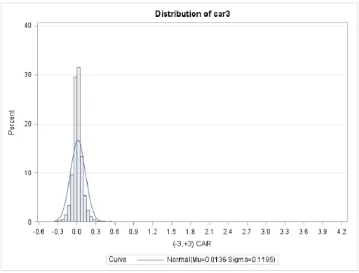
The dependent variable is the bidder’s CAR3 and for the sample the vast majority of the CAR3s are centered around on zero percent. Figure1 shows the distribution of CAR3 and figure 2 shows the probability plot of CAR3.
18 The mean is actually positive and equals 1.36% (and is statistically different from zero acording to the tests for location) for the sample with standard deviation of 11.95%. Most of the CAR3s are centered around zero, with the tails being very thin. The SAS code is in appendix A2.
Results Regression
The centerpiece of my analysis is a linear regression. The dependent variable CAR3 is the acquirer’s cumulative abnormal return for the whole period of between 3 days before and 3 days after the
announcement. CAR3 is fitted against the education concentration and other control variables to see how they impact CAR3 (SAS code for the regression in appendix A3).
The model:
CAR3 = β1*education concentration + β2*institutional concentration + β3*market size + β4*debt to market + β5*deal to market + β6*CEO centrality + β7*CEO tenure + β8*CEO tenure2 +
β9*total boards to date + β10*total current boards + β11*total current boards2 + β12*independent
past CFO + β13*board size + β14*board size2 + β15*intense monitor + β16*industry relatedness +
19 The description of the variables and their expected vs. their fitted signs are given in the following table:
Table 6
Independent variables description, fitted and expected relation with the CAR3
Variable Description Expected
sign
Fitted sign Education
Concentration The HHI-like variable for measuring the diversity of the board of directors’ education, a greater value implies less diversity Linear negative Linear negative Institutional
Concentration The HHI-like variable for measuring Block Holders ownership, a greater value implies greater ownership Linear positive Linear positive Market size The log of the market size of the acquirer at the moment of the
announcement Linear negative Insignificant Debt-to-market The ratio of the acquirer’s debt to its market value at the moment
of the announcement
Linear positive
Linear positive Deal-to-market The ratio of the value of the deal to the market value of the
acquirer at the moment of the announcement Linear positive Linear positive CEO centrality The number of directors from the Boardex dataset who have a
connection to the acquirer’s CEO at the moment of the announcement (shared school or work place)
Linear
negative Insignificant CEO tenure The amount of time the CEO has been in his position at the
moment of the announcement
Negative quadratic
Insignificant Total boards
To date The total number of boards that the acquirer’s directors sat on prior to the announcement, reflecting a “collective experience” and connections but also the ensuing power
Negative
quadratic Insignificant Total current
Boards The total number of boards that the acquirer’s directors sat on at the time of the announcement, reflecting board business Negative quadratic Insignificant Ind past CFO
fraction
The fraction of the independent directors to the total directors who have previously in their career held the position of a CFO
Unexplored Linear positive Ind past CFO The total number of the independent directors who have previously
in their career held the position of a CFO Unexplored Linear negative Board size The total number of directors of the acquirer at the moment of the
announcement Negative quadratic Negative quadratic Intense monitor Dummy variable equal to 1 if the majority of the independent
directors serve on at least 2 of the 3 principal monitoring committees.
Negative Negative Industry
relatedness A dummy variable equal to 1 if the acquirer’s and target’s first 3 digits of the 4 digit SIC code are the same Positive Negative PRIV A dummy variable equal to 1 if the target is a private company, as
compared to a public company Positive Positive Female Total number of female directors on the acquirer’s board at the
time of announcement Linear Positive Insignificant Duality A dummy variable equal to 1 if the CEO is also the chairman of the
board
20 And here are the regression results:
Table 7
Regressions results of the model. CAR3 is the dependent variable. *,**,*** means significance at 10%, 5% and 1% respectively
Variable Parameter Estimate t-value
Intercept 0.0082 0.22 education concentration -0.036 -2.41** institutional concentration 0.0414 3.61*** market size 0.0001 0.10 debt to market 0.0174 13.59*** deal to market 0.0549 30.31*** ceo centrality 0 0.49 ceo tenure -0 -0.16 ceo tenure2 0 1.12
total boards to date 0.0001 1.26
total current boards -0.0004 -0.69
total current boards2 -0 -0.27
independent past cfo fraction 0.13 2.42**
independent past cfo -0.0186 -2.91***
board size 0.0137 3.04***
board size2 -0.0006 -2.72***
intense monitor -0.0988 -3.24***
industry relatedness (sic3) -0.0054 -1.81* industry relatedness (sic2) -0.0063 -2.05**
Female -0.0004 -0.19
Duality -0.0013 -0.4
Priv 0.0356 7.7***
The variable education concentration is significant and negative, meaning that the more diverse is the board the greater in the acquirer’s CAR3. As a robustness check, I also estimated the model using the 6 category variables (6 dummies) as well as including the PhD and MBA variables (counting the total such degrees in the board) but all were insignificant. A dummy variable equal to 1 if the acquirer is a high tech company was also turned out to be insignificant.
In order to accept the results of the regression I tested whether the distribution of error terms are homoscedastic and normally distributed. Homoscedasticity describes a situation in which the error term (the difference between the actual data and the fitted data) is the same across all values of the independent variables, i.e has the same variance. Heteroscedasticity (violation of homoscedasticity) is present when
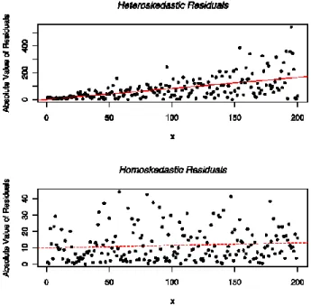
21 the size of the error term differs across values of the independent variables. When this occurs the areas with greater variance (as is demonstrated in figure 3) will have a greater pull on the fitted model than other observations and this is because the OLS is fitting the model with the smallest sum of squares of the error terms and since observations with greater variance have bigger errors their square term of the error will also be bigger and therefore the adjustment is more influenced by them. According to Berry and Feldman (1985) and Tabachnick and Fidel (1996) slight heteroscedasticity has little effect on significance tests, but when heteroscedasticity is large it can lead to serious distortion of the findings and increase the possibility of a Type I error (incorrect rejection of a true null hypothesis).
As an illustration, figure 3 shows a case of homoscedasticity and in it the fitted line is flat which could imply a true null hypothesis, but in the case of heteroscedasticity the line is pulled upwards which could imply a positive relation when there should be none.
Figure 2. Heteroscedasticity depiction
Testing for heteroscedasticity.
Two tests will be used to determine whether heteroscedasticity is present in the model: the Breusch-Pagan and Whites’s tests.
22 The Breusch-Pagan tests whether the estimated variance of the residuals from a regression is dependent on the values of the independent variables and if that is the case then heteroscedasticity is present. The test takes the squared residuals of the fitted model and fits them against the independent variables in a second auxiliary regression. The idea behind the test is that squared residuals from the original model serve as a proxy for the variance of the error term at each observation (the error term is assumed to have a mean of zero, and the variance of a zero-mean random variable is the expectation of its square). The independent variables in the auxiliary regression account for the possibility that the error variance depends on the values of the original independent variables in some linear way.
White’s test is similar to the Breusch-Pagan, with the addition that its auxiliary regression incorporates the squares and the cross products of the independent variables as well, and therefore is able to detect a more general form of heteroscedasticity.
The null hypothesis for both tests is that there is no heteroscedasticity in the original regression and the statistical hypothesis test is the Chi Square test (appendix A4 for the SAS code).
Table 8
Heteroscedasticity of the Errors Tests
Test Pr>ChiSq
White's Test <.0001
Breusch-Pagan <.0001
Both tests reject the null hypothesis of no heteroscedasticity.
Looking at the Residual vs CAR3 plot in figure 4 will give some visual idea on how the errors are distributed and how their variance varies across CAR3.
23 Figure 3. Residual vs CAR3 plot
It can be seen that there seems to be a linear “45 degree” relation between the residuals and CAR3s, and the variation increases as the CAR3 approaches 0. I tried several times to cut the tails by various degrees since the absolute value of the Student Residual increases with the absolute value of the residual, but heteroscedasticity was still present. The Studenstized Residual is the quotient of the division of a residual by an estimate of its standard deviation. The studentized residual is used to find outliers because the standard deviations of residuals in a sample can vary greatly between different points, even if the errors have the same stabdard deviation, so it is not completely correct to detect outliers simply by looking at the size of the residual.
Testing for Normality
Normality of the error terms is the other necessary assumption for a regression which is important for accurate calculation of the p – values and significance testing, although this assumption is not needed for the validity of the OLS model. When the errors are normal the OLS estimator is equivalent to the
Maximum Likelihood Estimator and is asymptotically efficient. When the sample size is large, it is possible to derive the asymptotic properties of the interval estimates of the model parameters even if we
24 don’t make any assumption about the distribution of the error term, by virtue of the Central Limit
Theorem. But I will do the normality tests nevertheless.
Three tests will be used to test for the normality of the errors: Kolmogorov-Smirnov, Cramer-von Mises and Anderson Darling.
The Kolmogorov-Smirnov test is a nonparametric test of the equality of continuous,
one-dimensional probability distributions that can be used to compare a sample with a reference probability distribution (one-sample K–S test), or to compare two samples (two-sample K–S test). The Kolmogorov– Smirnov statistic quantifies a distance between the empirical distribution function of the sample and the cumulative distribution function of the reference distribution, or between the empirical distribution functions of two samples. The null distribution of this statistic is calculated under the null hypothesis that the sample is drawn from the reference distribution (in the one-sample case) or that the samples are drawn from the same distribution (in the two-sample case). In the special case of testing for normality of the distribution, samples are standardized and compared with a standard normal distribution.
The Cramer-von Mises criterion is a criterion used for judging the goodness of fit of a cumulative distribution function compared to a given empirical distribution function , and in this case the cumulative distribution function of the errors is compared to the normal distribution.
The Anderson-Darling test is a statistical test of whether a given sample of data is drawn from a given probability distribution. In its basic form, the test assumes that there are no parameters to be estimated in the distribution being tested, in which case the test and its set of critical values is
distribution-free. When applied to testing if a normal distribution adequately describes a set of data, it is one of the most powerful statistical tools for detecting most departures from normality (Stephens, 1974). Tests for the normality of the error terms (appendix A5):
Table 9
Normality of the Errors Tests
Test p Value
Kolmogorov-Smirnov <0.01
Cramer-von Mises <0.005
Anderson-Darling <0.005
25 So the results from the regression are dubious because the assumptions of heteroscedasticity and
normality of the error terms are not met and therefore the inference about the model’s parameters and their significance are not conclusive.
Addressing the Heteroscedasticity Problem Box Cox Transformation
The Box-Cox (Box Cox, 1964) provides a family of transformations that will optimally normalize a particular variable, eliminating the need to randomly try different transformations to determine the best option. This is a useful data transformation technique used to stabilize variance and make the data more normal distribution-like
The one-parameter Box–Cox transformations are defined as:
The Box Cox transformation attempts to find the exponent (Lambda) for the y variable that will transform the data into a normal shape. The transformation is done using different Lambdas, and the best Lambda is the one that results in the smallest standard deviation of the data, although it is customary to use the “standard” Lambda (e.g -1, 0.5, 2 etc.) closest to the resulting Lambda. The transformation which results in the smallest standard deviation of the data by itself isn’t a guarantee for normality, but rather the transformed data has the highest likelihood of being normal when the standard deviation is the smallest, and might mitigate heteroscedasticity. Consider the example by King et al. (2014) that illustrates the Box-Cox transformation which also results in the error terms becoming homoscedastic:
26
Since about half of the CAR3s in the data are negative it is necessary to add a constant to the CAR3s before applying the transformation (a square root cannot be taken of a negative number for example). Osborne (2002) recommends anchoring at 1 (i.e, making the smaller value equal to 1) because numbers above 0.00 and below 1.0 behave differently than numbers 0.00, 1.00 and those larger than 1.00. The square root of 1.00 and 0.00 remain 1.00 and 0.00, respectively, while numbers above 1.00 always
27 become smaller, and numbers between 0.00 and 1.00 become larger. Since the smallest CAR is equal to -0.55 I will add 1.55 to the CARs.
Using SAS to calculate the best transformation we get λ=-1. So the newly transformed dependent variable becomes 1 – 1/(y+1.55). (SAS code is appendix A6).
But there is still heteroscedasticity according to the White and Breusch-Pagan tests, both giving a probability of less than 0.0001
FGLS
Feasible Generalized Least Squares is a special case of Generalized Least Squares. GLS is a technique for estimating the unknown parameters of a linear regression and making a heteroscedastic model into a homoscedastic one if the variance-covariance matrix of the error term is known.
Feasible Generalized Least Squares is a method used when there is heteroscedasticity but the variance of the error terms is unknown and has to be estimated. To estimate a FGLS model, I begin by extracting the error terms, u, from the original OLS regression. Then I assume that the error terms are a function of the independent variables and estimate a regression, by taking log on both sides, where the dependent variable is the estimated squared error term. Here are the steps taken from the lecture notes of Yamato (2009)
WLS (Weighted Least Squares) takes each observation and divides it by its variance (which is the value along the diagonal of the variance-covariance matrix) so as to standardise the variance and make it equal for all the observations and thus eliminating heteroscedasticity.
28 FGLS by itself is biased (that is, the mean of the sampling distribution of the estimator is not equal to the true parameter value), but for large samples it is asymptotically unbiased, so it’s consistent (meaning that the estimator converges to the true value as the sample size increases).
But this method resulted in R square being 0.014 and all variables having a reduced significance, including concentration which becomes insignificant, and heteroscedasticity is still present. Regressing CAR3 against the Independent Variables individually
As both the Box-Cox and FGLS approaches had not been successful in addressing the heteroscedasticity problem, I then regressed CAR3 on each independent variable individually and attested the
heteroscedasticity of the resulting residuals in order to in order to see which variables are responsible for the heteroscedasticity of the general model.
The variables that result in heteroscedastic errors when the CAR3 is regressed against them individually are: ln_mkt , lt_mkt, instown_hhi, deal_mkt.
It should be noted that these values are among the values with the highest significance in the original model.
When omitting these variables from the general model, White’s test gives a p value =1 and Breusch – Pagan test gives a value of 0.89, so the heteroscedasticity disappears, but the adjusted R square becomes 0.01 (although the F value is 4.99 which is significant at the 1% level). The concentration variable coefficient remains negative and significant as before, but the model explains very little of the total variance, less than 1%, whereas in my original model I had and adjusted R2 close to 30%, although previous papers studying the CAR around the announcement event had adjusted R2 ranging from 5% to 40%.
Flexible Functional Form
The persistent heteroscedasticty in the model prevents us from accepting the results of the OLS, but maybe the real model isn’t linear at all. A model is defined as nonlinear if the derivatives of the model with respect to the model’s parameters depend on one or more parameters. Nonlinear models are often derived on the basis of physical and/or biological considerations, e.g., from differential equations, and have justification within a quantitative conceptualization of the process of interest.
29 Since the form and the parameters of the nonlinear model are unknown a method to estimate them is the Flexible Functional Form:
yt(λ)
= β
1+ β
2x
2t(λ)+ … + + β
kx
kt(λ)where y
t(λ) = (ytλ – 1)/λ for λ ≠0 and ln(yt) otherwise.The general case is when all the lambdas are potentially different. The special case when lambdas =1 is a simple linear regression.
The method iteratively fits the model for different values of the parameters (given initial parameters and a range for Lambda) and calculates the sum of squares between the original data and the fitted model. The iterative process stops when the fit can no longer be improved (i.e, the sum of squares doesn’t get any smaller) and the fit is said to have converged.
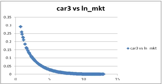
Solving the model is very computational intensive and beyond the means available to me (my computer crashed even for 2 variables) so for illustrative purposes I tried to fit a flexible functional form for the dependent variable CAR3 with the explanatory variable ln_mkt. I choose this variable because it was one of the variables that resulted in a heteroscedastic variance of the error term when the CAR3 was linearly fitted against them individually.
Car3 = (1+λ*intercept + λ*β
1*ln_mkt
λ)
1/λThis method besides being very computationally intensive is also very sensitive and gives different results for different ranges of possible parameters. For example, I estimated the model twice; in both estimates the starting values for intercept values are between 0.01 and 0.15 (with increment 0.01) and β1 are between 0.01 to 0.1 (increment of 0.01). In the first model Lambda is fitted between 0.5 to 2.5 (increment 0.5) and in the second case it is fitted between -2.5 to -0.5 (increment 0.5).
Figures 5 and 6 show the two nonlinear flexible models and table 8 the descriptive results of these fits (SAS code in appendix A7).
30 Figure 5. First non linear model
Figure 6. Second non linear model
Table 9
Summary of the first and second non-linear fits for CAR3 vs log of Market Size
iteration intercept B1 Lamda
Sum of squares First non-linear fit 29 0.0996 -1.2181 0.3481 67.3983 Second non-linear fit 100 -92.658 91.2566 -0.0171 67.83
0 0.05 0.1 0.15 0.2 0.25 0.3 0.35 0.4 0.45 0 5 10 15
car3 vs ln_mkt
car3 vs ln_mkt31 In both non-linear models the sum of squares is very similar (and for each case the coefficients are chosen so as to have the smallest sum of squares) and the curves are also similar, but all the coefficients are very different. Also note that the fitted parameters have different signs depending on the model, which makes it hard not only to choose the right model but also to interpret the meaning of the results.
Omitted Variable Bias
A reason for heteroskedasticity might be omission of variables from the model. As an illustration, consider the following graph:
Just by looking at the data points it seems that they have a quadratic shape, and the model
Y = α + β1X + β2X2 would nicely fit the data (the purple parabola) resulting in no heteroskedasticity. But if the quadratic term is omitted and the new model becomes Y = α + β1X (the red line) then there will be heteroskedasticity and it can be clearly seen by the greater dispersion of the data points as they get closer to the extremes.
Besides being a potential cause for heteroskedasticity, OVB can result in biased and inconsistent estimators. Consistency means that as the sample increases the estimators converge to their true value. For illustration, consider the true model:
Y = A + BX + CZ + u
If the covariance between X and Z is non-zero such that Z = D + FX + e, and variable Z is omitted from the original model, then the regression estimates the following model:
Y = (A+CD) + (B+CF)X + (u+Ce) and therefore the coefficient of the variable X is biased by CF in order to compensate for the omitted variable Z.
32 Heteroskedasticity consistent standard errors
The model might contain heteroskedsticity inherently. For example, if one looks at the graph of a household’s luxury expenditure fitted against its total income, there will be heteroskedasticity because households with a small income will spend little on luxury goods, whereas households with a big income might spend a lot or be more moderate with their spending, so the increased variability seen for high earning households is completely natural.
Heteroskedasticity might also be the result of the data being sampled from different populations. Consider the following graph, where there are data from a the blue and the red population, and each is
homoscedastic as seen by the dispersion around each respective fitted line, but if the model is not aware of this, then it will result in the black line fit which is heteroskedastic.
So instead of trying to correct for the heteroskedasticity, it could be assumed as inherent to the model. A method to deal with such a situation is using heteroskedasticity consistent standard errors (HCSE) and an