A Deep 3D Object Pose Estimation Framework for Robots with RGB-D Sensors

(1)

Worcester Polytechnic Institute

Digital WPI

Masters Theses (All Theses, All Years)

Electronic Theses and Dissertations

2019-04-24

A Deep 3D Object Pose Estimation Framework for

Robots with RGB-D Sensors

Ameya Yatindra Wagh

Worcester Polytechnic Institute

Follow this and additional works at:

https://digitalcommons.wpi.edu/etd-theses

This thesis is brought to you for free and open access byDigital WPI. It has been accepted for inclusion in Masters Theses (All Theses, All Years) by an authorized administrator of Digital WPI. For more information, please [email protected].

Repository Citation

Wagh, Ameya Yatindra, "A Deep 3D Object Pose Estimation Framework for Robots with RGB-D Sensors" (2019).Masters Theses (All Theses, All Years). 1287.

(2)

(3)

Abstract

The task of object detection and pose estimation has widely been done using template matching techniques. However, these algorithms are sensitive to outliers and occlusions, and have high latency due to their iterative nature. Recent research in computer vision and deep learning has shown great improvements in the robustness of these algorithms. However, one of the major drawbacks of these algorithms is that they are specific to the objects. Moreover, the estimation of pose depends significantly on their RGB image features. As these algorithms are trained on meticulously labeled large datasets for object’s ground truth pose, it is difficult to re-train these for real-world applications.

To overcome this problem, we propose a two-stage pipeline of convolutional neural net-works which uses RGB images to localize objects in 2D space and depth images to estimate a 6DoF pose. Thus the pose estimation network learns only the geometric features of the object and is not biased by its color features. We evaluate the performance of this frame-work on LINEMOD dataset, which is widely used to benchmark object pose estimation frameworks. We found the results to be comparable with the state of the art algorithms using RGB-D images. Secondly, to show the transferability of the proposed pipeline, we implement this on ATLAS robot for a pick and place experiment. As the distribution of images in LINEMOD dataset and the images captured by the MultiSense sensor on ATLAS are different, we generate a synthetic dataset out of very few real-world images captured from the MultiSense sensor. We use this dataset to train just the object detection networks used in the ATLAS Robot experiment.

(4)

Acknowledgements

I would like to thank Professor Michael A. Gennert, my thesis advisor for his valuable contribution throughout the journey of this thesis. I would like to thank Professor Emmanuel O. Agu and Professor Berk Calli for being part of the thesis committee. I would also like to thank Vinayak Jagtap for his guidance and support throughout the research. Lastly, I would like to thank my parents and my friends for the motivation and valuable support required throughout.

(5)

iv

List of Figures

2.1 Point cloud of a coffee mug . . . 4

2.2 Sample image and its corresponding depth image . . . 5

2.3 Object detection using feature histograms . . . 7

2.4 Viewpoint Feature Histogram of bowl and mug . . . 8

2.5 Visualization of predicted labels for objects in scene . . . 8

2.6 Segmentation masks projected on RGB images . . . 9

2.7 Object proposals in 3D space . . . 10

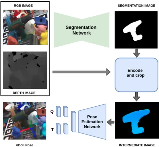
3.1 Proposed 2-stage pipeline consisting segmentation stage and pose estimation stage. Q in the figure stands for quaternion vector of dimension 4x1 and T stands for translation vector of dimension 3x1. . . 12

3.2 A sample image showing semantic segmentation and instance segmentation [38] 13 3.3 Architecture of Segnet [1] . . . 14

3.4 An RGB Image and a binary mask inferred from Segmentation network . . . 15

3.5 Pose estimation using EPnP [29] . . . 18

3.6 Registration of point clouds using Iterative Closest Point [13] . . . 19

3.7 Network architecture for object pose estimation . . . 20

3.8 Depth image (top left), its JET encoding representation (top right) and image after element-wise multiplication (bottom) . . . 21

3.9 Representation of object center in u,v coordinate space . . . 22

4.1 Image of Ape from Linemod dataset (left), corresponding segmentation masks(right) 28 4.2 Sample image and its augmentations used during training . . . 29

4.3 RGB images of ape, drill and bench-wise (left), their corresponding masks (Right). . . 31

4.4 Predicted and ground truth pose overlayed on the RGB images. The axes with a blob at the tip is the ground truth pose, the other is the predicted pose 33 4.5 Trends of accuracy with change in distance threshold for (from top left to bottom right) ape, benchvise, cam, can, cat, drill . . . 34

4.6 Trends of accuracy with change in distance threshold for (from top left to bottom right) duck, egg-box, glue, hole-punch, iron, lamp . . . 35

4.7 Images of the object captured with MultisenseSL . . . 37

(8)

4.9 Images of the Background captured with MultisenseSL . . . 38

4.10 Synthetically Generated Images . . . 38

4.11 Masks for Synthetically Generated Data . . . 39

4.12 MultiSense SL sensor used on the ATLAS robot [33] . . . 41

4.13 TOUGH API overview [9] . . . 42

4.14 Drill detection on Atlas Robot . . . 45

4.15 Drill detection on Atlas Robot . . . 46

4.16 Sequence of images from a video of pose estimation experiment . . . 47

4.17 From Top left to bottom right: object detected by the robot, planning and executing trajectory to grab the object, closing the gripper to grasp, returning to default pose . . . 48

(9)

viii

List of Tables

4.1 Segmentation Performance on LINEMOD Images . . . 30

4.2 Statistics of Segmentation Performance on LINEMOD Images . . . 30

4.3 Inference Speed on LINEMOD dataset . . . 36

4.4 Comparative Analysis of dataset distributions . . . 39

4.5 Segmentation Performance on Real world Images . . . 40

(10)

Chapter 1 Introduction

1.1 Problem Statement

The problem statement considered in this thesis is to develop a perception framework for robots which do not have sensors such as Kinect. A lot of algorithms being trained are sensor specific or object specific. These algorithms use color keypoint or features to match specific templates. The network gets biased to these features, thus making it specific to the object. On the contrary, depth images encode only the geometrical information of the object and can be used to predict the pose hypothesis. Secondly, deep neural networks are resource intensive and thus, making it difficult to implement in real-time robotics applications.

In this work, different methods of object detection and pose estimation are explored and a convolutional neural network based architecture is proposed which uses RGB features to localize the object and then uses geometric features from the depth image to predict the object pose. First, the framework is trained and evaluated on a publicly available LINEMOD dataset. Then, the object localization module of the same network is retrained on fewer images for a particular object and tested on a real robot with a different sensor for object pick-up task. The pose estimation network is not retrained in this experiment.

(11)

2

1.2 Related Work

The problem of recognizing an object and estimating its pose has been a topic of interest for years. This has a lot of applications in robotics, mainly in the manipulation of the object. There has been an exponential growth in research on processing 3D point cloud scenes. Conventional computer vision techniques do not work out of the box on point clouds. Hence, new methods for feature description and segmentation are being proposed.

Traditionally, template matching techniques are used, which compute correspondences between a 3D model and a point cloud scene [13, 3, 16, 18]. These correspondences are then scored using a similarity function and thus a pose hypothesis with the best score is chosen. These algorithms are either sampling based or iterative in nature which is inefficient in inference speed. Similarly, template matching techniques are used to match the projections of 3D models on 2D images [32], [20], [37], [23], [24], [27]. Although template matching techniques show great performance in estimating object pose, they heavily depend on image key points or features. With occlusions, the numbers of key points reduce and thus affects these methods significantly.

Alternately, feature based methods perform better in handling occlusions. They are used to compute local and global features, which act as a signature of the object of interest. These features are then matched with a 3D model to find the correspondences in the image. Meth-ods such as DLT [28] and E-PnP [29] are used traditionally to estimate a pose hypothesis by computing a relation between the 2D-3D key points.

With the massive success of Deep learning framework and increased precision in laser sensors, some end to end object recognition pipelines were proposed. Pose-CNN [40] is one such end to end network which uses Convolution neural networks and attempts to regress pose using just RGB images. Similarly, Deep-6D Pose [6] extends the Mask RCNN [14] framework to localize instances of objects and regress pose. IPose [19] uses similar instance segmentation network and leverages the depth image to obtain the object pose using geometrical methods. BB8 [32] uses a multilevel detection process in which they use VGG Network to detect object ROI and train a CNN on 2D projections of 3D objects to predict object pose. Another Multi-view approach by [42] uses multiple viewpoints to fit

(12)

pre-scanned 3D models to 2D segments of the object of interest.

1.3 Contribution

• Explored 2 approaches, a point cloud based approach and RGB-D based approach for detecting and localizing objects in 3D scenes.

• Proposed a 2 stage pipeline using Convolutional Neural Networks to infer 6 DoF pose of the object from RGB-D images

• Contributed to T.O.U.G.H, a C++ API library for humanoids research (main contri-butions are on tough perception package)

• Evaluated the proposed pipeline on LINEMOD dataset

• Experimentally validated the performance of the method for real-world application by implementing on ATLAS Robot.

1.4 Outline

The thesis is outlined as follows

• Chapter 2explores the point cloud based and RGB-D based approaches and builds a path for the proposed pipeline.

• Chapter 3gives an overview of each block of the proposed framework and dives deep into the implementation.

• Chapter 4 evaluates the proposed framework on LINEMOD dataset and ATLAS robot.

(13)

4

Chapter 2 Preliminary Experiments

2.1 Background

This section gives an overview of 2 different representation of 3D information. The point cloud representation and RGB-D representation is explained briefly in the following subsections.

2.1.1 Understanding Point cloud

Point clouds are a representation of data points of an object in 3D-space. Every point on the object is represented by the x,y,z coordinates with reference to the sensor frame.

(14)

As every individual point represents its position in the 3D space, a set of points describing a point cloud can be represented as Organized point cloud and Unorganized point cloud. An organized point cloud is represented as a 2D array similar to an image. This gives an advantage of computing graph based operations such as finding the nearest neighbor simpler and intuitive. Alternately, unorganized representation of point cloud structure is an array of points with their x,y,z values. Unorganized point cloud usually has dimensions such as Nx3 where N is the number of points and 3 is the dimension for [x,y,z] position vector. Moreover, points can also encode their color information and thus every point can be represented as [x, y, z, R, G, B]. Figure 2.1 shows a visualization of unorganized colored point cloud.

2.1.2 Understanding RGB-D Image

RGB-D is yet another representation of 3D objects. The RGB stands for the 3 color channels (RED, GREEN, BLUE) in the image. An additional depth channel is added to create a 4 channel image. Every pixel in the depth channel corresponds to the distance of the point from the image plane. In most cases, x and y-axes are on the image plane and z-axis is normal to the image. Thus, the z-values of the points are used to generate the depth image.

(a) RGB Image (b) Depth Image

Figure 2.2: Sample image and its corresponding depth image

Figure 2.2 shows an instance of the RGB image and its corresponding image. The depth image is normalized to [0-255] values for the ease of visualization in grayscale.

(15)

6

2.2 Preliminary Experimentation

To evaluate the feature-based method, the presented experiments consists of 2 ap-proaches. The first approach uses only the point cloud representation of the object and the second uses RGB-D representation. These experiments assume the use case of table-top scenarios and dense point clouds.

2.2.1 Approach 1: Point cloud only

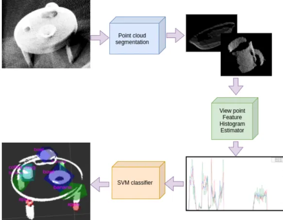
For the preliminary experimentation, multiple point cloud based approaches were tested on RGB-D Dataset [21]. To identify the objects in the scene, the point cloud scene was segmented into smaller point clouds using euclidean distance clustering. For every segment obtained, a global feature histogram was computed. Viewpoint Feature Histogram Estimator (VFHE)[35] is one of the techniques used to compute global features of a point cloud. The VFHE computes normals to every single point in the point cloud and angle of the normal with respect to the viewpoint vector. These angles are binned in 360 bins to form a feature vector. The RGB-D dataset [21] provides point cloud models of individual objects in the scene whose VFH can be used as ground truth. These histograms were used to train a Support Vector Machine (SVM)[15] classifier. At inference, this trained SVM was used to predict class labels for the segments obtained by euclidean distance clustering, see figure 2.3.

(16)

Figure 2.3: Object detection using feature histograms

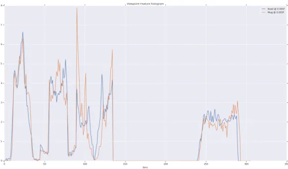
It was observed that symmetric objects such as mugs and bowls have similar feature histograms which confused the SVM classifier, refer to figure 2.4 . Moreover, it took ap-proximately 1-2 minutes to process the complete point-cloud on an i7 CPU with 16 GB Memory.

(17)

8

Figure 2.4: Viewpoint Feature Histogram of bowl and mug

The final results contained a lot of outliers due to over-segmentation and objects with symmetric geometry. Figure 2.5 shows the misclassified labels, where the edge of the table is detected as banana and the upper part of a cap is detected as a bowl.

(18)

2.2.2 Approach 2: RGBD

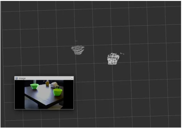
Another approach with 2D segmentation proposals was tested 2.6 which performed better on symmetric objects. A SegNet [1] model pre-trained on ImageNet[5] was used to detect 2D segmentation masks, which were used as region proposals. These masks were then projected onto the aligned depth images to obtain a crop of the depth image. Using the camera intrinsics provided, this depth image was projected back into 3D space, reconstructing point clouds of the objects 2.7.

Figure 2.6: Segmentation masks projected on RGB images

Despite noise in the depth image, the point cloud generated closely resembled the actual object and the detection was significantly faster.

(19)

10

Figure 2.7: Object proposals in 3D space

The segmentation mask is a binary image which indicates pixels belonging to the object and background, whereas the depth image contains the distances of individual points from the image plane. By performing element-wise multiplication of the depth image with the segmentation mask, only the pixels corresponding to the objects have non-zero depth values. Using the camera intrinsic matrix, these depth images are converted into point clouds. Figure 2.7 shows a visualization of the reconstructed point cloud in RViZ software [10].

2.2.3 Conclusion

From the above experiments [2.2.1, 2.2.2], It can be concluded that the projection based method performs better than the point cloud only method. The RGB images play an important role in localizing the object. Based on these results, a 2-stage object pipeline is proposed which can localize objects and estimate their 6DoF pose. The RGB images are limited to the segmentation stage as the segmentation networks can be trained for new objects using techniques such as transfer learning.

(20)

Chapter 3 Methodology

3.1 System Overview

The object detection and pose estimation pipeline is divided into two stages, an RGB image segmentation network and an object pose estimation network. The object segmen-tation network is a more generic module and can be swapped with any state of the art binary image segmentation convolutional neural network. The contribution of this research is mainly towards developing a light-weight Convolutional Neural Network which predicts object pose as a pair of a position vector and a quaternion vector. As the framework is implemented on a machine connected to the actual robot with limited computational power (6GB VRAM), two large networks on Single GPU could not be accommodated. Thus, the model architecture is limited to smaller networks which agree with the inference speed and accuracy trade-offs. These computation specifications are only limited to the inference stage while the training is done on a large cluster of CPUs and GPUs.

(21)

12

Figure 3.1: Proposed 2-stage pipeline consisting segmentation stage and pose estimation stage. Q in the figure stands for quaternion vector of dimension 4x1 and T stands for translation vector of dimension 3x1.

(22)

3.2 2D Image Segmentation

This section builds the foundation to understand semantic segmentation in 2D images. The architecture of SegNet and the changes made are discussed in the following.

3.2.1 Understanding Image segmentation

Semantic segmentation is an approach to partition image pixels into groups of similar context. Unlike the object detection algorithms which draw a bounding box around an object, semantic segmentation algorithms use pixel-wise labeling strategies to indicate pixels of a similar class or an object. Semantic segmentation is widely used in scene understanding.

Figure 3.2: A sample image showing semantic segmentation and instance segmentation [38]

Classical computer vision techniques perform semantic segmentation by separating the foreground and background. These methods are mainly categorized as Layer-based and block-based segmentation. The layer based techniques consist of banks of filters in order to define binary masks for the objects, whereas the block-based methods use information from various features of the image to collectively generate segmentation masks. A review paper [41] elaborates these techniques in detail.

With the advancement in deep learning and especially deep convolutional neural net-works, there has been a significant improvement in the accuracies as well as inference speed of these segmentation algorithms. A general deep segmentation architecture consists of an encoder and a decoder. This encoder is a set of convolution layers and downsampling layers stacked together in descending order of dimensions. The output of the encoder is a high di-mensional representation of the image which only encodes the most significant information.

(23)

14

The decoder, on the other hand, takes this information and tries to reconstruct this image as a binary image. This binary image is the segmentation mask in which the object pixels are distinguished from the background. A more in-depth review of the state of the art deep learning algorithms for semantic segmentation is discussed by [12].

3.2.2 SegNet

SegNet [1] follows an encoder-decoder architecture consisting of multiple layers of con-volutional neural networks. The encoder uses the first 13 convolution layers from VGG-16 network. VGG [36] models are deep convolutional neural network architectures which per-formed significantly well on ImageNet challenge [5]. In this way, the encoder can be initial-ized with pre-trained VGG16 weights, which gives the network a better starting point in the training process. The last layer of the encoder contains all the high-dimensional information of the image which is later used to reconstruct a segmentation mask.

Figure 3.3: Architecture of Segnet [1]

The SegNet differs from other networks by its decoder architecture. The decoder is a mirror image of the encoder except the Pooling layers are replaced by up-sampling. SegNet stores the indices of the values during max-pooling and uses them in the decoder stage to up-sample in the same way as it was down-sampled. This way it saves a lot of memory without much loss of accuracy.

(24)

3.2.3 Implementation of 2D segmentation network

As this segmentation block is generic, a Vanilla SegNet architecture with minor changes was used. A dropout layer was introduced after every convolution block in the encoder and decoder stage to avoid over-fitting. A standard dimension of 640x480 was chosen as input to the network with mean - normalized images. The output layer is a single channel probability map with softmax output. This softmax output is converted to a binary segmentation map using a threshold of 0.5. The loss function is a combination of Binary Cross Entropy Loss and a custom loss function which penalized Intersection over Union 3.26.

SegNet was chosen because of its performance and speed. For more accuracy, networks like U-Net [34] and Deep-Lab [4] perform better. For instance segmentation, MASK-RCNN [14] can be used to generate segmentation proposals and pose estimation network can iterate over all the proposals to find the object poses respectively.

(25)

16

3.3 Object Pose estimation

This section builds the foundation to understand pose estimation. Later, the architecture of the pose estimation network is discussed in detail.

3.3.1 Understanding Object Pose Estimation

Estimating the pose of given objects from the 2D image is generally done by computing a relationship between the 2D image coordinates and the 3D point coordinates. In this approach, the model is projected on an image plane with multiple poses and the projected image is matched with the original to select the pose with least error. Similarly, a 3D approach uses object models and computes a transformation between the scene and the model using registration algorithms like Iterative closest point.

Direct Linear Transform

The Direct Linear transform is the simplest and one of the early algorithms used to esti-mate the camera pose from 2D image key-points by estimating the homography matrices [7] [28] [29]. For a simplified 2D image the 2D world coordinates of the objects can be converted to u,v co-ordinates using the homography matrix given by 3.1. The x,y,z coordinates are the translations in x,y,z axes with respect to the camera frame. Whereas, the u,v coordinates are location of the pixels on an image plane with respect to the top left corner of the image.

c·      u v 1      =H·      x y 1      (3.1)

where H is given by 3.2 and c is a scalar non-zero constant.

H =      h1 h2 h3 h4 h5 h6 h7 h8 h9      (3.2)

The above equation 3.1 can be written in the formA·h= 0, where A is given by stacking 3.3, 3.4 to form A matrix 3.5 and h matrix by 3.6.

(26)

−h1·x−h2·y−h3 + (h7·x+h8·y+h9)·u= 0 (3.3) −h4·x−h5·y−h6 + (h7·x+h8·y+h9)·v= 0 (3.4) A=   −x −y −1 0 0 0 u·x u·y u 0 0 0 −x −y −1 v·x v·y v   (3.5) h= h h1 h2 h3 h4 h5 h6 h7 h8 h9 iT (3.6) The solution toA·h= 0is usually found out by Single Value Decomposition.It computes the eigen values of covariance and eigen vectors of A and returns solution along principal axis corresponding to minimum singular value [29]. Other optimization techniques based on different cost-functions are described in [7].

Perspective n Points - PnP

For estimating the homography matrix for 3D point, the homography matrix is repre-sented as a combination of camera intrinsic and extrinsic matrix 3.7.

c·      u v 1      =      fx 0 cx 0 fy cy 0 0 1      ·      R11 R12 R13 Tx R21 R22 R23 Ty R31 R32 R33 Tz      ·         x y z 1         (3.7)

When there are n sets of 3D-points with their 2D correspondences and known camera intrin-sics, the pose of the object w.r.t to the camera can be found out using Perspective n Points or PnP algorithm. PnP can be implemented as an iterative or non-iterative algorithm with at least 3 correspondence points. EPnp [22] is a variant of PnP which gives a solution in O(n) time complexity and is non-iterative. It represents a point as the weighted sum of 4 virtual non-coplanar control points, explained in equation 3.8. See figure 3.5.

(27)

18

Figure 3.5: Pose estimation using EPnP [29]

pw_i = 4

X

i=1

αi,j·cwj (3.8)

wherepw_i = [XwYwZw]T is a 3D point in world co-ordinate system andcw_j = [XwYwZw]T

is a 3D control point.

Similarly, using DLT in the control point reference frame, object pose is obtained [29].

Iterative closest Point

Iterative Closest Point is a registration algorithm, which computes a transformation matrix consisting of rotation and a translation of the object with respect to a given model of that object in the sensor frame [26]. The algorithm first computes distinct features in the model point cloud and the scene point cloud. These features are matched using feature matching algorithms to find correspondences.

(28)

Figure 3.6: Registration of point clouds using Iterative Closest Point [13] dk = 1 N N X i=1 ||yk−(Rk·xk+Tk)|| (3.9)

Wheredk gives the error distance in the sampled point yk and the modeled pointxk

trans-formed byRk rotation matrix and Tk translation matrix.

This process is iterated until the convergence criteria is satisfied. Following are the steps: • compute the correspondences to findyk and xk

• compute the registration using equation 3.9 and Singular value decomposition. • register the model in the scene using the transformations computed

• if dk < ek (where ek is some error threshold), return the transformations else repeat

the same for next iteration.

It is generally observed that ICP works best if it is provided with some initial estimate of the object pose, thus making it a good candidate for pose refinement. The coarse pose can be computed by the above mentioned methods like PnP.

(29)

20

3.3.2 Implementation of Pose Estimation Network

The above mentioned methods are good estimators of pose but are very prone to outliers and due to their iterative nature, they are time consuming. In this section, a deep learning architecture is described which learns the transformation of the objects points (represented as depth image) from the camera frame.

A VGG-11 encoder is modified by adding two fully connected regression networks to it. Thus, the network gives two output vectors, a 4x1 quaternion vector for the object pose and a 3x1 vector for location of the center of the object in a 3D co-ordinate space. At every forward pass the quaternion is normalized to make it a unit quaternion.

Figure 3.7: Network architecture for object pose estimation

ˆ

q= qˆ

|q| (3.10)

The segmentation mask obtained from the previous stage is used to crop out the depth values corresponding to the object. A square bounding-box is then fitted around the cropped depth image and resized to (224 x 224). The resultant image obtained is a square with only the depth values of the corresponding object.

As this is a single channel image, this information is encoded into 3 channels using a JET encoding. JET representation encodes the information in depth image into RGB space

(30)

which makes it structurally similar to an RGB image. The depth values in the depth image are normalized and are up-sampled to form a 3 channel 8 bit image. The points with lesser depth value are green in color and the values which are farther are red. See figure 3.8

JET encoding is proven to be helpful in object detection tasks with depth as additional data [8]. As the VGG11 encoder was pre-trained on ImageNet dataset, transfer learning with JET encoded depth images do not change the weights drastically.

Figure 3.8: Depth image (top left), its JET encoding representation (top right) and image after element-wise multiplication (bottom)

Pose estimation loss function is defined in [39] which estimates the loss as the Euclidean distance between sample points of the object which are transformed by predicted pose and its corresponding ground truth pose. Details of the loss function are discussed in 3.4.2

To infer the position of the object the position regression fully connected branch of the network regresses a 3x1 vector. As addressed by [40], the naive approach of regressing pose as 3D coordinates (x,y,z) of the center of the object cannot be generalized and is prone to errors. It would also depend on the image dimensions and camera intrinsics. To overcome this problem the position of the object center is represented in (u,v,z) coordinate representation.

(31)

22 x= (u−cx)·z fx (3.11) y= (v−cy)·z fy (3.12)

Figure 3.9: Representation of object center in u,v coordinate space

The top left co-ordinates of the bounding box were stored (ub, vv) before cropping the

depth image. The network regresses the center of the object (u0,v0, z), whereu0and v0are normalized co-ordinates of the object center with respect to the bounding-box.

u=ub+s·u0 (3.13)

v=vb+s·v0 (3.14)

where s is the side of the bounding box. u0 and v0 are normalized distance and can change from 0.0 to 1.0.

(32)

The rotation matrix is computed from the quaternion using the equation 3.15 and simi-larly translation matrix from the equation 3.16. These mathematical operations are imple-mented as tensors using pyTorch which gives the ability to perform these computations on a GPU. R=      1−2(q_y2+q_z2) 2(qx·qy−qz·qw) 2(qx·qz+qy·qw) 2(qx·qy +qz·qw) 1−2(qx2+q2z) 2(qy·qz−qx·qw) 2(qx·qz−qy·qw) 2(qy·qz+qx·qw) 1−2(qx2+qy2)      (3.15) T =hx y z iT (3.16)

3.4 Loss Function

This section discusses about the Loss functions in detail used in the segmentation network as well as in the pose estimation network.

3.4.1 2D segmentation loss

Binary Cross Entropy

The segmentation map generated by the segmentation network is a probability map of pixels belonging to the object. Thus, in a perfectly inferred segmentation map, the pixels belonging to the object will have a value close to 1.0 and the pixel belonging to the background will have values close to 0.0. Binary Cross Entropy Loss (BCE) computes the cross-entropy between the ground truth label distribution and the predicted label probability distribution. As the raw neural network values can be outside the range of 0.0-1.0, the output is normalized using a sigmoid function. 3.17

pi =

expesi

PN

j expesj

(3.17) Herepiis the softmax output ofithpixel andsi is the raw inferred value of the network.

BCE=−1 N N X i=0 (yilog( ˆyi) + (1−yi) log((1−yˆi))) (3.18)

(33)

24

Where N is the number of pixels in an mxn image, N = m×n, y is the ground truth label andyˆis the predicted softmax value of that pixel.

Example: Computing Binary Cross Entropy

Consider an image of dimension 3x3. The ground truth labels corresponding to the object is given by 3.19.      0 1 1 0 1 1 0 0 0      (3.19)

Similarly a predicted map is obtained from the Segmentation Network given by 3.20 which represents the probabilities with which the pixel belongs to the object.

     0.12 0.90 0.76 0.09 0.89 1.00 0.22 0.54 0.61      (3.20)

The Binary Cross Entropy loss is computed between the ground truth 3.19 and 3.20 by the equation 3.18.

Fori= 0,

BCE0 =−1·(0·log(0.12) + (1−0)∗log(1−0.12)) = 0.127

Accordingly computing BCE for i=0 to i=8 and then summing them up,BCE =−2.695

is obtained.

Intersection over Union

Intersection over Union (IoU) is a metric to evaluate the overlap of ground truth and predicted segmentation masks. As the overlap of the predictions over ground truth needs to maximized, a function of IoU as loss function is used.

IoU = |A∩B |

(34)

Example: Intersection over unionAfter a binary threshold operation with threshold value of τ = 0.5,a binary label map is obtained given by 3.22

     0 1 1 0 1 1 0 1 1      (3.22)

For the ground truth 3.19 and predicted mask 3.22 the intersection is given as 3.23 and Union is given as 3.24      0 1 1 0 1 1 0 0 0      (3.23)      0 2 2 0 2 2 0 1 1      (3.24) IoU is computed as IoU = Intersection U nion = 4 10 = 0.4 (3.25)

2D Segmentation Loss function

The final loss function used for training the segmentation network is given by 3.26 which incorporates both binary cross entropy loss and Intersection over union as a weighted sum. As IoU varies from 0.0 −→ 1.0 −log(IoU) changes from inf −→ 0.0 respectively. Thus, lower the IoU, higher is the loss.

(35)

26

3.4.2 Pose Estimation Loss

To train the Pose estimation network, a loss function defined in [39] is used, which tries to minimize the euclidean distance between ground truth and predicted point on the object.

Lpose= 1 M M X j=0 ||(Rxj +t)−( ˆRxj + ˆt)|| (3.27)

A set of M points are randomly sampled from the object (xj) and transformed with

the ground truth transformation matrix given by [R|T]. Similarly the same points are transformed with their corresponding transformation predicted by the network. Here the transformation[ ˆR|Tˆ]is obtained by converting the (u,v,z) co-ordinates to world co-ordinates using 3.13 , 3.14 , 3.15 and 3.16.

(36)

Chapter 4 Experimentation and Results

4.1 Experimentation and Evaluation on LINEMOD dataset

4.1.1 LINEMOD Dataset

Linemod [17] dataset is commonly used to benchmark object pose estimation algorithms. It consists of around 18000 images and ground truth pose for 15 different objects. The RGB images and corresponding depth images were captured using the Kinect sensor under indoor lighting conditions. All images are resized to 640x480 and are stored in jpg format. The dataset consists of the following files

• RGB images - 640x480 saved in jpg format

• distance.txt - contains maximum diameter of object in cm.

• transform.dat - contains the ground truth pose of the object as an SO4 transformation. • OLDmesh.ply - object mesh

• mesh.ply - object mesh after registration.

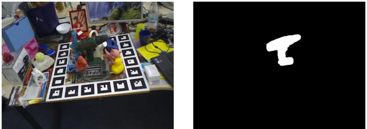
As the Linemod dataset does not provide pixel-wise segmentation masks, the object points from the ’mesh.ply’ files which were transformed according to the ground-truth pose were projected onto the images plane to generate a binary mask.

(37)

28

Figure 4.1: Image of Ape from Linemod dataset (left), corresponding segmentation masks(right)

4.1.2 Data augmentation

Deep neural networks often require large samples of the dataset to train. It is difficult to generate new image samples from the same image distribution. To overcome this problem image augmentation is used to generate more sample of images from the same distribution of images. A library albumentation [2] was heavily used to augment images to generate fake images. Following are the augmentations used in the training pipeline in an inline manner. The probability of the augmentation signifies that the chances of it being picked as an augmentation while pre-processing an image.

• One of (RandomContrast, MedianBlur, RandomBrightness) - probability(0.5) • VerticalFlip - probability(0.5)

• HorizontalFlip - probability(0.5) • ShiftScaleRotate - probability(0.5)

(38)

(a) Original Image (b) Horizontal Flip (c) Vertical Flip (d) Shift Scale Rotate

(e) Median Blur (f) Random Brightness (g) Random Contrast

Figure 4.2: Sample image and its augmentations used during training

4.1.3 Training

Both the convolutional networks are implemented in PyTorch[25] and used GPU for training. The segmentation network was trained from scratch using Adam optimizer with a learning rate of 1e−4and for 200 epochs. To avoid over-fitting it was empirically found out that a dropout rate of 0.1 worked well. The loss function used to optimize this network is defined in 3.26. Similarly, the pose estimation network uses Stochastic Gradient Descent optimizer and a learning rate of1e−4. The network was initialized with pre-trained weights trained on ImageNet dataset provided by PyTorch framework. The loss function used to optimize this network is defined in 3.27.

4.1.4 Segmentation Results

The accuracy of the segmentation network is evaluated with Jaccard Index, also know as Intersection over Union.

IoU = |pbin∩g|

(39)

30

wherepbin is the binary value of the predicted mask after performing a binary threshold

on the sigmoid output at 0.5. pbin ∈ {0,1}. g is the binary ground truth mask

Table 4.1: Segmentation Performance on LINEMOD Images

Objects IoU ape 0.944 benchvise 0.931 cam 0.929 can 0.938 cat 0.922 driller 0.928 duck 0.923 eggbox 0.931 glue 0.929 holepuncher 0.942 iron 0.931 lamp 0.922

Segmentation Performance on LINEMOD Images

Table 4.2: Statistics of Segmentation Performance on LINEMOD Images

Mean STD

0.9308 0.006

Average segmentation performance on LINEMOD Images

Table 4.1 shows IoU scores for all the 12 categories. The network shows an average IoU score of 0.9308 and a very low standard deviation which indicates robustness of the performance, refer table 4.2.

(40)

Figure 4.3: RGB images of ape, drill and bench-wise (left), their corresponding masks (Right).

4.1.5 Pose Estimation Results

To evaluate the accuracy of the final pose regressed by the Pose estimation network, Average distance metric is used proposed by [17]. A random point is sampled from the object and transformed with ground truth pose to obtain xg. The same point is then

transformed with the predicted pose to obtain a point xp. The error in the ground truth

pose and predicted pose is given by the Euclidean distance betweenxg and xp. refer 4.1.

d= 1 M M X j=0 ||(Rxj+T)−( ˆRxj+ ˆT)|| (4.1)

For a given thresholdτ (in cms). If the distance is less then a given threshold, The pose is accepted else the pose is rejected 4.2.

(41)

32 f =      1 d≤τ 0 otherwise (4.2)

The pose which is accepted is considered as a hit and the pose which is rejected is considered as miss. The accuracy of the model is computed by 4.3

accuracy= hit

(hit+miss) (4.3)

Figure 4.4 shows the ground truth pose and predicted pose of samples in the test set. The axes with a blob at the tip represents ground truth pose, whereas the other represents the predicted pose. These poses are projected on the original image for visually understand the results.

The pose estimation network was evaluated on varying distance thresholds for its accu-racy response. Figures 4.5, 4.6 shows the trend of accuaccu-racy vs the distance threshold. It can be observed that the distance accuracies are more than 90% when the threshold is greater than 30% of the object diameter. Moreover, the error values are large, this is due to its symmetry. There can be multiple valid pose for symmetric objects.

Comparing with BB8 [32], the pose accuracy of BB8 is more than 90% for threshold as 20% of the object diameter. The proposed approach does not perform well against BB8 as only depth information is used and no RGB features are learnt.

(42)

Figure 4.4: Predicted and ground truth pose overlayed on the RGB images. The axes with a blob at the tip is the ground truth pose, the other is the predicted pose

(43)

34

Figure 4.5: Trends of accuracy with change in distance threshold for (from top left to bottom right) ape, benchvise, cam, can, cat, drill

(44)

Figure 4.6: Trends of accuracy with change in distance threshold for (from top left to bottom right) duck, egg-box, glue, hole-punch, iron, lamp

(45)

36

Inference time

Table 4.3 shows the split of inference time of individual stages. The framework takes an average of 22.7 milliseconds for a forward pass. This is due to the smaller network size and light-weight architectures. Both the networks fit on one GTX 1060Ti GPU on which the performance was measured.

Table 4.3: Inference Speed on LINEMOD dataset

Stage Time

Segmentation 22.1 msec

Pose Estimation 5.7 msec

Total 27.8 msec

Average speed in milli-seconds for segmentation and pose estimation stage

4.2 Experimentation and Evaluation on ATLAS Robot

4.2.1 Acquiring Real World Images

The data distribution of RGB images of LINEMOD dataset is not similar to the images captured from the Multisense SL[33], refer table 4.4. This is because the camera intrinsic and the camera response curves of Multisense SL are different from that of Kinect sensor. Thus a network trained on LINEMOD images fails to perform well on images captured from other sensors.

To overcome this problem a custom segmentation dataset was created. Around 40 RGB images were captured using the multisense SL sensor with a drill machine as the object of interest, placed at different positions in the scene, refer figure 4.7. These 40 images with the object were annotated for pixel-wise segmentation masks. Refer figure 4.8.

(46)

Figure 4.7: Images of the object captured with MultisenseSL

(47)

38

Similarly, around 40 images of the background were captured by moving the sensor randomly, refer figure 4.9

Figure 4.9: Images of the Background captured with MultisenseSL

A python script generated a dataset of 4500 image samples by cropping the objects using the ground truth segmentation marks and randomly placing it on a background image which also were chosen randomly. The above mentioned data augmentations (refer 4.1.2) were also performed online to generate more samples from the distribution.

(48)

Figure 4.11: Masks for Synthetically Generated Data

Table 4.4: Comparative Analysis of dataset distributions

Dataset Mean R Mean G Mean B STD R STD G STD B LINEMOD IMAGES 0.333 0.333 0.332 0.191 0.191 0.190

REAL IMAGES 0.181 0.203 0.241 0.213 0.211 0.214 Mean and standard deviations of the R,G and B channels of normalized images in LINEMOD and REAL image dataset

Table 4.4 clearly shows the difference in the distribution of pixel values in R, G and B. LINEMOD dataset is captured in a very controlled lighting condition and can be seen from the standard deviations of the 3 channels, whereas the standard deviation of the images captured from the MultiSense sensor is higher. It can be observed that the mean RED value is significantly less than Green and Blue, which can be observed in the images in 4.7 and 4.9.

(49)

40

Table 4.5: Segmentation Performance on Real world Images

Fold IoU 0 0.944 1 0.932 2 0.948 3 0.936 4 0.929

Segmentation Performance on Real world Images

Table 4.6: Statisitcs of Segmentation Performance on Real world Images

Mean STD

0.9378 0.0071

Average segmentation performance on real world im-ages

To train the segmentation network this dataset was split into 5 folds each of80%training samples and 20%validation samples. The training procedure remained same as mentioned in 4.1.3. The table 4.5 and 4.6 shows no signs of over fitting as the IoU scores are consistent across all the folds.

4.2.2 Acquiring Depth Images

The primary sensor of ATLAS Robot is MultiSense SL [33]. It consists of a stereo camera pair and a spinning Hokuyo lidar, refer figure 4.12. Thus, there are 2 ways to obtain depth images, one from Hokuyo lidar scans and another from stereo image disparity. A point cloud fetched from a laser sensor can be projected on the image plane, the distance of the point from the plane is used as the value corresponding to the pixels of the depth image. Similarly, disparity images can be converted to depth images using the equation 4.4

(50)

The point cloud generated by the Lidar takes 1 rotation per 2.5 seconds to update. This is very slow and distorts the point cloud if the object is moved during the laser scan. On the other hand, the point cloud generated from the disparity image is observed to be noisy. As the pose estimation is not affected significantly by occlusions and noise, the depth maps are generated using disparity images obtained from the sensor.

(51)

42

4.2.3 TOUGH

The Atlas robot is configured to work with IHMC Controllers (version 0.11) which use ROS kinetic as an interface. TOUGH APIs [9] is a high-level C++ API library to con-trol the robot. It was developed at WPI Humanoid Robotics Lab to serve as a research framework for fast prototyping of software and algorithms on humanoid robots supported by IHMC controllers. This framework was tested on robots such as Valkyrie and ATLAS in simulation as well as on Physical robots. The API framework consists of multiple packages for controllers, motion planners, perception and navigation, refer 4.13. A graphical user interface is provided to quickly control the robot manually or monitor its states.

Figure 4.13: TOUGH API overview [9]

The scope of this research uses TOUGH Motion planning package for planning and execution of trajectories in the object pick-up experiment.

4.2.4 ROS nodes

To use the object detection and pose estimation pipeline with the ATLAS Robot, ROS-kinetic [31] is used as a platform to communicate with the Robot. Two ROS nodes are created, one to detect the object and one to manipulate and grab the object. The object detector node consists of a subscriber which listens to the image and depth message topics from multisense SL directly and pre-processes images into RGB and the depth image formats

(52)

respectively. For this particular task RGB and depth, images need to be synchronized and are done by using ApproximateT imeSynchronizerclass of "message filter" package which is available in ROS. The subscriber callback updates a global placeholder for RGB image and Depth depth and race conditions are avoided using Mutex locks.

Algorithm 1 Drill Detection node

1: procedure_{IMAGE_DEPTH_SYNC_SUBSCRIBER}(image_msg, depth_msg) . RGB image and depth images are synchronized and stored

2: RGB_image←decode(image_msg) 3: Depth_image←decode(depth_msg)

4: procedure_{ROS_LOOP}() .ROS node continuously running

5: whileROS6=shutdowndo

6: segmentation_mask ←SegmentationM odel(RGB_image)

7: object_pose←P oseEstimationM odel(Depth_image, segmentation_mask)

8: object_pose←M ovingAverageF ilter(object_pose) 9: broadcastObjectP ose(object_pose)

The ROS Loop implements the main algorithm of object detection and pose estimation. Both the segmentation and pose estimation network models run on GPU and need multi-threaded workers to load and fetch images from the GPU. This is handled by IO functions in PyTorch Library. First, the RGB image is passed to the Segmentation model to gener-ate a pixel-wise binary mask. The Pose Estimation Model uses the binary mask and the corresponding depth image to infer the object pose. As the output of the neural networks are not stable and have significant noise, the object pose is seen to jitter. This adds the problem when planning trajectories with TOUGH. To filter the noise in the detected object pose, A Moving average filter is used with a window size of 15. This window size was found out empirically and has less latency and noise.

(53)

44

Algorithm 2 Drill Manipulation node

1: procedure_{OBJECT_POSE_SUBSCRIBER}(object_pose_msg) . Listern to object pose being broadcasted

2: object_pose←decode(object_pose_msg)

3: procedure_{ROS_LOOP}() .ROS node continuously running

4: whileROS6=shutdowndo

5: waitF orU ser()

6: T OU GH.planT rajectory(object_pose)

7: visualizeT rajectory()

8: approval←waitF orU serApproval()

9: if approvalthen

10: T OU GH.executeT rajectory()

Drill Manipulation Node is fairly simple and leverages the high-level APIs provided by TOUGH. A Pose subscriber listens to the objects pose being broadcasted asynchronously. ROS Loop is implemented in an interactive manner where at every stage human approves the action. TOUGH runs Move-it planners (cite moveit) which converts the task space trajectories into joint space trajectories. The executeT rajectory procedure converts the trajectory points into the appropriate message and send it to the robot for execution.

(54)

Figure 4.14: Drill detection on Atlas Robot

Figure 4.14 shows the network architecture to communicate with the ATLAS Robot. A separate gigabit Ad-HoC network is created to have high bandwidth while communicating with the robot. Only the operator control units and 3 onboard ATLAS computer can com-municate over this network. As the network is not wireless, the possibility of the connection drops during the experimentation is eliminated. The ATLAS robot runs the ROS master node and IHMC controller on the onboard computers and listens to high levels commands by the TOUGH APIs running on other OCUs. The object detection node runs on an OCU with a GTX-Titan (2012 model with 6GB memory) whereas manipulation node is running on another OCU with the operator in the loop. The logger is used to log all the data being sent to or received from the robot which is then used to analyze the experiment later in time.

(55)

46

4.2.5 Drill Detector Task

To demonstrate the functioning of the algorithm on Atlas robot, a drill is kept in front of the Robot and at a reachable location. The drill detection node listens to the RGB images and depth images being published by the MultiSense sensor on the robot and estimates a 6DoF pose. This pose is published as a ROS Pose message. A ROS message of transform is also published for the sake of visualization. Fig 4.15 shows a view of RViz, a visualization software for ROS. The left image in the RViz shows the colored point cloud and the pose of the drill being detected in the scene, whereas the right image shows the RGB image from the left camera and an overlayed segmentation mask.

Figure 4.15: Drill detection on Atlas Robot

To verify the performance of the system visually on a moving object, the object was moved randomly in the field of view of the robot. Fig 4.16 shows a sequence of frames of a video. The left image in each frame is the 3D colored point cloud and the image on the right is the RGB image with the segmentation mask overlaid on top. It can be noted from the figure that the segmentation mask sometimes detects random objects as the drill or multiple

(56)

proposals. To fix this issue, only the proposal which has the largest area is considered.

Figure 4.16: Sequence of images from a video of pose estimation experiment

Although the pipeline works very fast on the dataset as a standalone application, The integration with ROS and the use of an older GPU due to the limitations of the hardware connected with the Robot limits the performance. A Total average inference speed of 250 msec was obtained which is approximately 4Hz. This is a decent speed for any manipulation and planning frameworks to plan for trajectories.

(57)

48

4.2.6 Drill Pick-up Task

The drill Pick-up task is an extension of the drill detection task. This experiment is performed with a human in loop to verify every stage of the task being done correctly and approve the decisions made by the robot during the experiment.

Figure 4.17: From Top left to bottom right: object detected by the robot, planning and executing trajectory to grab the object, closing the gripper to grasp, returning to default pose

In this experiment, the robot was initialized and calibrated, and put into STAND mode as the purpose of this experiment was only to manipulate the object and not to navigate around. The drill object was kept at a reachable distance with proper safety precautions taken during the high power and high pressure was activated. The experiment was conducted with a 7 DoF and a 10 DoF planner. For the 7Dof planner experiment, the object was placed close to the robot and could be easily picked. In pick-up task, the robot first detected the

(58)

object and its pose. It then planned a trajectory and waited for the user to approve for execution. Once the action was approved it moved the arm to the given pose and grasped the object. The operator then approved the grasps and approved return to home pose. refer 4.17

Out of 5 trials 4 were successful and 1 failed due to the error in the achieved task space position of the end-effector. This can be caused due to an error in the plan or errors in the intrinsic sensor such as joint encoders.

Figure 4.18: Failing to continuously detect object with 10DoF planning experiment

(59)

50

was placed at a farther distance than the previous experiment such that the robot plans a trajectory using all the 10 torso joints. As the object was stationary the robot was able to detect and pick up the object but the experiment failed in continuously detecting the object. As the robot reaches to grab the object, it’s head turns away from the object and out of the field of view for the object. Thus the network starts to give random values for 6DoF Pose which can be seen in 4.18. The robot still achieves a perfect grasp but would fail if the object moved during the execution of the task.

(60)

Chapter 5 Conclusion

5.1 Conclusion

In this work, two feature-based approaches were evaluated on the basis of their infer-ence speed and accuracy. The approach with point cloud segmentation and using feature histograms to detect objects was observed to be affected by the symmetry of objects and outliers. Moreover, the segmentation of the point cloud took significant time to process which makes it inefficient for real-time applications. On the contrary, the projection based method was significantly faster and was able to extract object point clouds from the scene with very less false positives.

Based on the Conclusions derived from chapter 2, A 2 stage Convolutional Neural Net-work architecture was proposed which leverages the projection based approach. A pose estimation network was developed and evaluated on LINEMOD dataset to benchmark the performance of the pipeline.

To test the transferability of the framework, the proposed pipeline was used on a real ATLAS robot for object pick-up task. As the distribution of images in LINEMOD and the images captured by the MultiSense were different, a small dataset was created to fine-tune the object localization network which uses semantic segmentation proposals. The segmentation network shows no signs of over-fitting and gives an accuracy (IoU) of 0.9378 on the real world images. The pipeline is observed to work well for 4 out of 5 experiments

(61)

52

of detecting and picking up an object. It was observed that the pose network gives random values when the object is not present in the field of view. Thus, it cannot be directly used in closed loop manipulation frameworks.

(62)

Chapter 6 Future Work

• Pose Estimation Network: The projection based network needs a lot of pre-processing and is dependent on the spatial organization of information i.e organized point cloud. Some information is lost when the depth image is downsampled. This can be overcome by using a point cloud processing architectures such as PointNet[30] to directly regress the object pose.

• Training and validation on YCB dataset YCB[11] dataset contains multiple household objects with its ground truth pose and segmentation masks. As the dataset contains multiple masks and their instances, the SegNet can be replaced with an in-stance segmentation network such as MASK-RCNN [14]

• Data generation with pose labels: The dataset generated by combining and aug-menting images from multisense sensor does not contain pose information. A more elaborate dataset can be generated by using a 3D model of the object and randomly translating in the scene. The projection of the object after translation can then be used to generate masks automatically. This will enable an end-to-end training of new architectures. Capturing the model of the object in itself can be a turntable experi-ment.

(63)

54

Appendix A

Appendix

A.1 TOUGH API description

Source code for simplified version of manipulation node used for object pick-up experi-ment using ATLAS Robot.

1 #i n c l u d e < p l u g i n l i b / c l a s s _ l o a d e r . h> 2 #i n c l u d e <r o s / r o s . h> 3 #i n c l u d e < t f / t f . h> 4 #i n c l u d e <geometry_msgs / PoseStamped . h> 5 #i n c l u d e "tough_common/tough_common_names . h" 6 #i n c l u d e " to ug h _m ov e it _p l an n er s / t a s k s p a c e _ p l a n n e r . h" 7 #i n c l u d e " t o u g h _ c o n t r o l l e r _ i n t e r f a c e / w h o l e b o d y _ c o n t r o l _ i n t e r f a c e . h" 8 #i n c l u d e <t o u g h _ c o n t r o l l e r _ i n t e r f a c e / g r i p p e r _ c o n t r o l _ i n t e r f a c e . h> 9 #i n c l u d e < s t d l i b . h> 10#i n c l u d e <std_msgs / S t r i n g . h> 11#i n c l u d e <tough_common/tough_common_names . h> 12 13 W h o l e b o d y C o n t r o l I n t e r f a c e∗ w b _ c o n t r o l l e r ; 14 C h e s t C o n t r o l I n t e r f a c e∗ c h e s t _ c o n t r o l l e r ; 15 A r m C o n t r o l I n t e r f a c e∗ a r m _ c o n t r o l l e r ; 16 T a s k s p a c e P l a n n e r∗ p l a n n e r ; 17 R o b o t D e s c r i p t i o n∗ rd_ ; 18 G r i p p e r C o n t r o l I n t e r f a c e∗ gc_ ; 19 geometry_msgs : : PoseStamped g o a l ;

(64)

20 21 b o o l RUN_STATUS = t r u e; 22 23 enum c l a s s PLANNER{ 24 7DOF, 25 10DOF 26 } ; 27

28 b o o l movetoPose (c o n s t s t d : : s t r i n g planning_group , geometry_msgs : : PoseStamped&

g o a l ) 29 { 30 moveit_msgs : : R o b o t T r a j e c t o r y t r a j e c t o r y _ m s g ; 31 i f ( p l a n n e r−>g e t T r a j e c t o r y ( g o a l , planning_group , t r a j e c t o r y _ m s g ) ) 32 { 33 w b _ c o n t r o l l e r−>e x e c u t e T r a j e c t o r y ( t r a j e c t o r y _ m s g ) ; 34 r e t u r n t r u e; 35 } 36 r e t u r n f a l s e; 37 } 38

39 v o i d poseCB ( geometry_msgs : : PoseStamped &msg ) 40 { 41 g o a l = msg ; 42 } 43 44 v o i d w a i t F o r U s e r ( ) 45 { 46 i n t c h o i c e ; 47 s t d : : c o u t << " P r e s s 0 t o a b o r t , P r e s s any o t h e r key t o c o n t i n u e . . " << s t d : : e n d l ; 48 s t d : : c i n >> c h o i c e ; 49 i f ( c h o i c e ==0) 50 RUN_STATUS = f a l s e; 51 } 52 53 i n t main (i n t a r g c , c h a r∗∗ a r g v ) 54 {

(65)

56 55 r o s : : i n i t ( a r g c , argv , " m o t i o n _ p l a n n i n g _ t u t o r i a l ") ; 56 r o s : : A s y n c S p i n n e r s p i n n e r ( 1 ) ; 57 s p i n n e r . s t a r t ( ) ; 58 r o s : : NodeHandle nh ; 59 60 r o s : : S u b s c r i b e r sub = nh . s u b s c r i b e (" d r i l l _ d e t e c t o r ", 1 0 0 0 , poseCB ) ; 61 62 w b _ c o n t r o l l e r = new W h o l e b o d y C o n t r o l I n t e r f a c e ( nh ) ; 63 p l a n n e r = new T a s k s p a c e P l a n n e r ( nh ) ; 64 c h e s t _ c o n t r o l l e r = new C h e s t C o n t r o l I n t e r f a c e ( nh ) ; 65 a r m _ c o n t r o l l e r = new A r m C o n t r o l I n t e r f a c e ( nh ) ; 66 rd_ = R o b o t D e s c r i p t i o n : : g e t R o b o t D e s c r i p t i o n ( nh ) ; 67 gc_ = new G r i p p e r C o n t r o l I n t e r f a c e ( nh ) ; 68 69 R o b o t S i d e i n p u t S i d e = R o b o t S i d e : : RIGHT ; // R i g h t hand u s e d 70 PLANNER planner_ = PLANNER : : 7 DOF; // 7DoF p l a n n e r u s e d 71 s t d : : s t r i n g p l a n n i n g _ g r o u p ; 72 gc_−>o p e n G r i p p e r ( i n p u t S i d e ) ; 73 w a i t F o r U s e r ( ) ; 74 75 w h i l e (RUN_STATUS) 76 { 77 i f ( i n p u t S i d e == R o b o t S i d e : : LEFT) 78 { 79 i f ( planner_==PLANNER : : 7 DOF) 80 { 81 p l a n n i n g _ g r o u p . a s s i g n (TOUGH_COMMON_NAMES: : LEFT_ARM_7DOF_GROUP) ; 82 } 83 e l s e 84 { 85 p l a n n i n g _ g r o u p . a s s i g n (TOUGH_COMMON_NAMES: : LEFT_ARM_10DOF_GROUP) ; 86 } 87 } 88 e l s e 89 { 90 i f ( planner_==PLANNER : : 7 DOF) 91 {

(66)

92 p l a n n i n g _ g r o u p . a s s i g n (TOUGH_COMMON_NAMES: : RIGHT_ARM_7DOF_GROUP) ; 93 } 94 e l s e 95 { 96 p l a n n i n g _ g r o u p . a s s i g n (TOUGH_COMMON_NAMES: : RIGHT_ARM_10DOF_GROUP) ; 97 } 98 } 99 gc_−>o p e n G r i p p e r ( i n p u t S i d e ) ; 100 w a i t F o r U s e r ( ) ; 101 movetoPose ( planning_group , g o a l ) ; 102 w a i t F o r U s e r ( ) ; 103 gc_−>c l o s e G r i p p e r ( i n p u t S i d e ) ; 104 w a i t F o r U s e r ( ) ; 105 a r m _ c o n t r o l l e r−>moveToDefaultPose ( s i d e , 3 . 0 ) ; 106 c h e s t _ c o n t r o l l e r−>r e s e t P o s e ( ) ; 107 } 108 // c l e a n−up 109 d e l e t e w b _ c o n t r o l l e r ; 110 d e l e t e c h e s t _ c o n t r o l l e r ; 111 d e l e t e a r m _ c o n t r o l l e r ; 112 d e l e t e p l a n n e r ; 113 d e l e t e rd_ ; 114 d e l e t e gc_ ; 115 }

(67)

58

Bibliography

[1] Vijay Badrinarayanan, Alex Kendall, Roberto Cipolla, and Senior Member. SegNet : A Deep Convolutional Encoder-Decoder Architecture for Image Segmentation. Arxiv, pages 1–14, 2017.

[2] Alexander Buslaev, Alex Parinov, Eugene Khvedchenya, Vladimir I. Iglovikov, and Alexandr A. Kalinin. Albumentations: fast and flexible image augmentations. Arxiv, 2018.

[3] Zhe Cao, Yaser Sheikh, and Natasha Kholgade Banerjee. Real-time scalable 6DOF pose estimation for textureless objects. Proceedings - IEEE International Conference on Robotics and Automation, 2016-June:2441–2448, 2016.

[4] Liang Chieh Chen, George Papandreou, Iasonas Kokkinos, Kevin Murphy, and Alan L. Yuille. DeepLab: Semantic Image Segmentation with Deep Convolutional Nets, Atrous Convolution, and Fully Connected CRFs. IEEE Transactions on Pattern Analysis and Machine Intelligence, 40(4):834–848, 2018.

[5] J. Deng, W. Dong, R. Socher, L.-J. Li, K. Li, and L. Fei-Fei. ImageNet: A Large-Scale Hierarchical Image Database. In CVPR09, 2009.

[6] Thanh-Toan Do, Ming Cai, Trung Pham, and Ian Reid. Deep-6DPose: Recovering 6D Object Pose from a Single RGB Image. Arxiv, 2018.

[7] Elan Dubrofsky. Homography Estimation. Opt. Eng., 15(March):977, 2009.

(68)

Wolfram Burgard. Multimodal deep learning for robust RGB-D object recognition.

IEEE Int. Conf. Intell. Robot. Syst., 2015-Decem:681–687, 2015. [9] Jagtap V. et. al. Tough. GitHub repository, 2019.

[10] William Woodall. et. al. rviz. GitHub repository, 2019. [11] et. al. Berk Calli. YCB Object Set. online, 2015.

[12] Alberto Garcia-Garcia, Sergio Orts-Escolano, Sergiu Oprea, Victor Villena-Martinez, and Jose Garcia-Rodriguez. A Review on Deep Learning Techniques Applied to Se-mantic Segmentation. Arxiv, pages 1–23, 2017.

[13] Philipp Glira. Iterative closest point (icp), 2016. Last accessed 11 April 2019.

[14] Kaiming He, Georgia Gkioxari, Piotr Dollar, and Ross Girshick. Mask R-CNN. Proceed-ings of the IEEE International Conference on Computer Vision, 2017-October:2980– 2988, 2017.

[15] Marti A. Hearst. Support vector machines. IEEE Intelligent Systems, 13(4):18–28, July 1998.

[16] Stefan Hinterstoisser, Cedric Cagniart, Slobodan Ilic, Peter Sturm, Nassir Navab, Pas-cal Fua, and Vincent Lepetit. Gradient response maps for real-time detection of tex-tureless objects. IEEE Trans. Pattern Anal. Mach. Intell., 34(5):876–888, May 2012. [17] Stefan Hinterstoisser, Cedric Cagniart, Slobodan Ilic, Peter Sturm, Nassir Navab,

Pas-cal Fua, and Vincent Lepetit. IEEE TRANSACTIONS ON PATTERN ANALYSIS AND MACHINE INTELLIGENCE 1 Gradient Response Maps for Real-Time Detec-tion of Texture-Less Objects. IEEE TRANSACTIONS ON PATTERN ANALYSIS AND MACHINE INTELLIGENCE, pages 1–14, 2012.

[18] Stefan Hinterstoisser, Vincent Lepetit, Slobodan Ilic, Stefan Holzer, Gary Bradski, Kurt Konolige, and Nassir Navab. Model based training, detection and pose estimation of texture-less 3d objects in heavily cluttered scenes. In Kyoung Mu Lee, Yasuyuki

(69)

60

Matsushita, James M. Rehg, and Zhanyi Hu, editors, Computer Vision – ACCV 2012, pages 548–562, Berlin, Heidelberg, 2013. Springer Berlin Heidelberg.

[19] Omid Hosseini Jafari, Siva Karthik Mustikovela, Karl Pertsch, Eric Brachmann, and Carsten Rother. iPose: Instance-Aware 6D Pose Estimation of Partly Occluded Objects.

Arxiv, 2017.

[20] Wadim Kehl, Fabian Manhardt, Federico Tombari, Slobodan Ilic, and Nassir Navab. SSD-6D: Making RGB-Based 3D Detection and 6D Pose Estimation Great Again. Pro-ceedings of the IEEE International Conference on Computer Vision, 2017-Octob:1530– 1538, 2017.

[21] Kevin Lai, Liefeng Bo, Xiaofeng Ren, and Dieter Fox. A Large-Scale Hierarchical Multi-View RGB-D Object Dataset. Arxiv, 2011.

[22] Vincent Lepetit, Francesc Moreno-Noguer, and Pascal Fua. EPnP: An accurate O(n) solution to the PnP problem. Int. J. Comput. Vis., 81(2):155–166, 2009.

[23] David G. Lowe. Object Recognition from Local Scale-Invariant Features. Arxiv, pages 35–40, 1999.

[24] Frank Michel, Alexander Kirillov, Eric Brachmann, Alexander Krull, Stefan Gumhold, Bogdan Savchynskyy, and Carsten Rother. Global Hypothesis Generation for 6D Object Pose Estimation. CVPR, pages 462–471, 2016.

[25] Adam Paszke, Sam Gross, Soumith Chintala, Gregory Chanan, Edward Yang, Zachary DeVito, Zeming Lin, Alban Desmaison, Luca Antiga, and Adam Lerer. Automatic differentiation in pytorch. online, 2017.

[26] Neil D. McKay Paul J. Besl. A Method for Registration of 3-D Shapes. online, 1992. [27] Georgios Pavlakos, Xiaowei Zhou, Aaron Chan, Konstantinos G. Derpanis, and Kostas

Daniilidis. 6-DoF object pose from semantic keypoints. Proceedings - IEEE Interna-tional Conference on Robotics and Automation, pages 2011–2018, 2017.

(70)

[28] Thomas Petersen. A Comparison of 2D-3D Pose Estimation Methods. Master’s thesis, Aalborg Univ. Media Technol. Comput. Vis. Graph. Lautrupvang, 15:2750, 2008. [29] Edgar Riba Pi, Francesc Moreno, Noguer Adrián, and Peñate Sanchez. Universitat

Poli ecnica de Catalunya Implementation of a 3D pose estimation algorithm. online, 0(June), 2015.

[30] Charles R. Qi, Hao Su, Kaichun Mo, and Leonidas J. Guibas. PointNet: Deep Learning on Point Sets for 3D Classification and Segmentation.CVPR2017, pages 601–610, 2017. [31] Morgan Quigley, Ken Conley, Brian Gerkey, Josh Faust, Tully Foote, Jeremy Leibs, Rob Wheeler, and Andrew Y Ng. Ros: an open-source robot operating system. In

ICRA workshop on open source software, volume 3, 2009.

[32] Mahdi Rad and Vincent Lepetit. BB8: A Scalable, Accurate, Robust to Partial Oc-clusion Method for Predicting the 3D Poses of Challenging Objects without Using Depth. Proceedings of the IEEE International Conference on Computer Vision, 2017-October:3848–3856, 2017.

[33] Carnegie Robotics. MultisenseSL. https://carnegierobotics.com/, 2012.

[34] Olaf Ronneberger, Philipp Fischer, and Thomas Brox. U-net: Convolutional networks for biomedical image segmentation. Lecture Notes in Computer Science (including subseries Lecture Notes in Artificial Intelligence and Lecture Notes in Bioinformatics), 9351:234–241, 2015.

[35] Radu Bogdan Rusu, Gary Bradski, Romain Thibaux, and John Hsu. Fast 3D recog-nition and pose using the viewpoint feature histogram. IEEE/RSJ 2010 International Conference on Intelligent Robots and Systems, IROS 2010 - Conference Proceedings, pages 2155–2162, 2010.

[36] Karen Simonyan and Andrew Zisserman. Very Deep Convolutional Networks for Large-Scale Image Recognition. pages 1–14, 2014.

[37] Bugra Tekin, Sudipta N. Sinha, and Pascal Fua. Real-Time Seamless Single Shot 6D Object Pose Prediction. Arxiv, 2017.

A Deep 3D Object Pose Estimation Framework for Robots with RGB-D Sensors

Worcester Polytechnic Institute

Digital WPI

Masters Theses (All Theses, All Years)

Electronic Theses and Dissertations

2019-04-24

A Deep 3D Object Pose Estimation Framework for

Robots with RGB-D Sensors

Ameya Yatindra Wagh

Follow this and additional works at:

https://digitalcommons.wpi.edu/etd-theses

Repository Citation

Abstract

Acknowledgements

Contents

List of Figures

List of Tables

Chapter 1

Introduction

1.1

Problem Statement

1.2

Related Work

1.3

Contribution

1.4

Outline

Chapter 2

Preliminary Experiments

2.1

Background

2.2

Preliminary Experimentation

Chapter 3

Methodology

3.1

System Overview

3.2

2D Image Segmentation

3.3

Object Pose estimation

3.4

Loss Function

Chapter 4

Experimentation and Results

4.1

Experimentation and Evaluation on LINEMOD dataset

4.2

Experimentation and Evaluation on ATLAS Robot

Chapter 5

Conclusion

5.1

Conclusion

Chapter 6

Future Work

Appendix A

Appendix

A.1

TOUGH API description

Bibliography