Time series forecasting of styrene price using a hybrid ARIMA and neural network model

(1)

[http://creativecommons.org/licenses/by/3.0/us/]

Licensed under a Creative Commons Attribution 3.0 United States License

915

TIME SERIES FORECASTING OF STYRENE PRICE USING A HYBRID ARIMA AND NEURAL NETWORK MODEL

Ali Ebrahimi Entekhab Industial Group, Iran, Islamic Republic of E-mail: aliebrahimi64@gmail.com Submission: 23/09/2018 Revision: 25/09/2018 Accept: 23/10/2018

ABSTRACT

Every player in the market has a greater need to know about the smallest change in the market. Therefore, the ability to see what is ahead is a valuable advantage. The purpose of this research is to make an attempt to understand the behavioral patterns and try to find a new hybrid forecasting approach based on ARIMA-ANN for estimating styrene price. The time series analysis and forecasting is an essential tool which could be widely useful for finding the significant characteristics for making future decisions. In this study ARIMA, ANN and Hybrid ARIMA-ANN models were applied to evaluate the previous behavior of a time series data, in order to make interpretations about its future behavior for styrene price. Experimental results with real data sets show that the combined model can be most suitable to improve forecasting accurateness rather than traditional time series forecasting methodologies. As a subset of the literature, small number of studies has been done to realize the new forecasting methods for forecasting styrene price.

Keywords: ARIMA; Hybrid ARIMA-ANN; Artificial neural networks; Time series forecasting

(2)

916

1. INTRODUCTION

Styrene is an unsaturated liquid hydrocarbon gained as a petroleum by-product. Also known as ethylbenzene, vinyl benzene, and phenyl ethane that is an organic compound with the chemical formula C6H5CH=CH2 (ENERGY, 2013). It is easily polymerized and is used to make plastics and resins (YOUSIF, 2013). A few of the most familiar uses of styrene include: Solid and film polystyrene, used in rigid foodservice containers, CD cases, appliance housings; Polystyrene foam, used in food service products and building insulation; Composite products, used in tub and shower enclosures and many other applications (CIECIERSKA, 2015).

The miscellaneous types of factors have been causing directly on the price of the styrene move up and down; exchange rates, feedstock price increases, strong demand, poor availability and even storms in the US (SHERMAN, 2010). These lead to an extensive risk and ambiguity in the process of price forecasting. The key player needs reliable forecasts of predictable styrene price in order to make the correct decision. This results in increased price variability and accords prominence to reliable price forecasting methods. The styrene price forecasts are so important for the manufacturer in order to production planning and marketing planning decisions on the predictable prices, which may have financial impacts in future months.

The price data analysing has become more complex under the modern market today. The main goal of the study is to find a technique that improves the forecasting estimate. Therefore, numerous types of methods and methodologies can be used. Time series forecasting is an imperative area of forecasting in which past observations of the same variable are collected and analysed to develop a model describing the underlying relationship (ZHANG, 2003).

Time series based models like Autoregressive Integrated Moving Average (ARIMA) and Artificial Neural Networks (ANN) are favoured when time series of historical prices are used. The styrene price data contain both linear and nonlinear patterns, no single model is capable to identify all the characteristics of time series data. Thus, in this study, ARIMA, ANN time series models and hybrid of both ARIMA and ANN models were used to model and forecast the price of styrene.

These methods undoubtedly lack the ability to catch all price spikes or price decreases in order to changes in important drivers but offer a way to have a constant

(3)

917

expectation of tomorrow’s power prices (Ozozen, 2016). By merging different

methods, the problem of model selection can be made better with little extra work. There is a long discussion about which methods are more efficient. Although more than a few comparative studies have been labelled in the literature, the findings do not suggest what circumstances make a method better than another. Therefore, situations of difficulty, seasonality, and perishability, require analytical studies about the most suitable method for each condition.

This paper is organized as follows. In the next section, we review the ARIMA and ANN modelling approaches to time series forecasting. The new proposed combination methodology explains in Section 3. Empirical results from real data sets are reported in Section 4. Section 5 contains the concluding remarks and future work respectively.

2. THEORETICAL BACKGROUND 2.1. Styrene

Figure 1 shows the main method of making styrene from ethane (derived from natural gas reserves) or naphtha (a product mainly derived from crude oil). Ethane (or naphtha) with steam is fed into the cracker unit where ethylene and coproducts (propylene, butadiene, benzene, etc.) are made. The ethylene and benzene are then further processed (catalytic alkylation) to make ethylbenzene from the cracker. This is then fed into a dehydrogenation reactor to make styrene (with minor coproduct benzene and toluene). The styrene is then typically piped to other chemical plants where it is further processed into derivative products such as polystyrene (ICIS, 2015).

(4)

918

Figure 1: Manufacturing Process of Styrene Monomer

Source: Miyashita (2012)

2.2. ARIMA Model

The ARIMA (Autoregressive Integrated Moving Average) model was popularized by George Box and Gwilym Jenkins in the 1970s, with use in time series analysis and forecasting. The underlying theories described by Box and Jenkins and later by Box, Jenkins and Reinsell are sophisticated but easy to understand and apply (DA VEIGA, 2014). The “I” in ARIMA implies that the dataset undergoes differentiation and that, upon completion of the modelling, the results undergo an integration process to produce final predictions and estimates (TULARAM, 2016). It is a combination of three statistical models. It uses Autoregressive, Integrated and Moving Average (ARIMA) model for statistical information (JAIN, 2017).

The ARIMA model has been widely studied and applied in researches of forecast in order to their attractive theoretical attributes and because of the many empirical supportive pieces of evidence. In addition, the ARIMA model has equivalence with most models of exponential smoothing (DA VEIGA, 2014). The ARIMA Model analyse and Forecasts uniformly spaced univariate statistic information, transmission of function data, and intercession information that is done by using Autoregressive Integrated Moving Average (JAIN, 2017).

The first thing to do in ARIMA is to determine the stationarity. It is a common assumption in many time series techniques. The probability laws governing the process do not change over time. The process is in statistical equilibrium. Besides, a

(5)

919

stationary process has the property that the mean, variance and auto covariance

structure do not change over time (RUSIMAN, 2017).

This method has some interesting features that made it more desirable for researchers. It eases the forecasting process allowing researchers to use only single variable time data series while also allow multiple for more complex cases (BARI, 2015). Also, the main advantage of this class of models lies in its ability to quantify random variations present in any economic time series (DAREKAR, 2016).

(NEWAZ, 2008) and (AHMAD, 2013) have applied ARIMA model based on which they predict can provide well forecasts. In another contribution, (MADDEN, 2007) has addressed the forecasting of gold prices through ARIMA model and had concluded by proposing that the gold selling prices are in increasing trends and could be deliberated as a worthy investment. (AS' AD, 2012) devised ARIMA Models based past three, six, nine and twelve months of data and advised that the ARIMA model build based on past three months' data is the best model in terms of forecasting. (LIM, 2001) and (DA VEIGA, 2014) figure out that the ARIMA methodology performs fairly well in their studies.

2.3. ANN Model

The conception of artificial neural networks (ANN) has been used for almost 50 years, only in the late 1980s could one determine that it gained significant use in scientific and technical performances (HAMID, 2004). ANN is a mathematical model that has a greatly connected structure similar to brain cells. A neural network is a machine that is designed to model the way in which the brain does a specific task. It resembles the brain in two respects: 1. Knowledge is attained by the network from its environment through a learning procedure; 2. Interneuron connection strengths, identified by synaptic weights, are applied to store the acquired knowledge (YADAV, 2017).

Artificial neural network (ANN) methods have shown great capability in modelling and forecasting nonlinear and complex time series. ANN offers an effective approach for handling large amounts of dynamic, nonlinear, and noise data (SHABRI, 2014). Neural networks, with their incredible ability to derive meaning from complex or imprecise data, can be used to extract patterns and identify trends that are too complex to be observed by either humans or other computational methods.

(6)

920

Other advantages include 1. Adaptive learning: An capability to learn how to do tasks

based on the data set as training or initial experience. 2. Self-Organization: An ANN can create its own organization or representation of the information it receives during learning time. 3. Real-Time Operation: ANN computations may be carried out in parallel, and special hardware devices are being designed and manufactured which take advantage of this capability (YADAV, 2017).

ANN is developed based on biological neural networks that neurons are the fundamental building blocks ones. An artificial neuron is a model of a biological neuron as you see in Figure 2. An artificial neuron receives signals from other neurons, gathers these signals, and when fired, transmits a signal to all connected neurons (MOMBEINI, 2015).

Figure 2: Biological model of a neuron Source: neuron (2016)

An ANN model frequently contains three layers: the first layer is the input layer where the data are announced to the network, the network is executed by using electric modules or in software on a digital computer simulation. The second layer is the hidden layer where data are processed, and the last layer is the output layer where the results of the given input are produced (SHABRI, 2014).

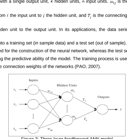
An important step in the neural network is to train the model to learn the relationship between input and output parameters. In multilayer perceptron (MLP), weights are determined by Error Back-Propagation (EBP) algorithms which minimize a quadratic cost function by a gradient descent method. The interconnecting weights between the neurons are adjusted based on the inputs and desired output during the training phase (GODARZI, 2014). The most popular and successful model is the feed forward multilayer network. Figure 3 shows a three-layer feedforward neural

(7)

921

network with a single output unit, hidden units, input units. is the connection

weight from the input unit to the hidden unit, and is the connecting weight from the hidden unit to the output unit. In its applications, the data series is usually divided into a training set (in sample data) and a test set (out of sample). The training set is used for the construction of the neural network, whereas the test set is used for measuring the predictive ability of the model. The training process is used essentially to find the connection weights of the networks (PAO, 2007).

Figure 3: Three-layer feedforward ANN model

Numerous papers have already presented the successful application of ANN for modelling and price forecasting. (MOVAGHARNEJAD, 2011) used ANN and a time variable as a constant variable; thus the dynamic nature of the process was not accounted for. (YU, 2008) stated that the performance of the ANN is superior to various traditional statistical models. ANN has a capability to learn complicated and nonlinear time series that is problematic to model with conventional models. However, there are some weaknesses of ANN. (YOUSEFI, 2015) concluded that using wavelet transform can enhance the forecasting accuracy when it is compared with a regular neural network prediction algorithm. (KHASHEI, 2011) concluded that Although ANN has advantages of accurate forecasting, their performance in some specific situation is inconsistent. (AHMAD, 2001) and (PAO, 2007) and (PANELLA, 2012) show that artificial neural network provided more accurate predictions.

(8)

922

In the past two decades, ANN and ARIMA (ANN-ARIMA) techniques widely

applied to achieve high accuracy forecasting's in linear and non-linear domains respectively; especially to forecast financial data onto the different type of economic and financial conditions (RATHNAYAKA, 2015).

Nevertheless, none of them is a general model that is appropriate for all circumstances. The estimate of ARIMA models to complex nonlinear problems might not be acceptable. On the other hand, using ANNs to model linear problems have yielded mixed results (ZHANG, 2003). For instance, via simulated data, (DENTON, 1995) indicated that when there are outliers or multi-collinearity in the data, neural networks can significantly outperform linear regression models.

(ZHANG, 2003) stated that it is more effective to combine individual forecasts that are based on different information sets. Also (NAVEENA, 2017) concluded that the hybrid method which combines linear and non-linear models can be an effective way to improve forecasting performance. (RATHNAYAKA, 2015) suggested that the hybrid model is more significant and gives the best solution for predicting future predictions under the high volatility fluctuations than traditional forecasting approaches.

3. DATA AND METHODS

The well-known datasets - Reed Business Information (ICIS) - is used in this study to determine the effectiveness of the hybrid method. ICIS is the world's biggest petrochemical market data provider with divisions spanning energy and fertilizers. The data we collected from the official websites of ICIS contains the daily number of styrene prices from 11/21/2005 to 9/19/2017, providing a total of 3002 sample values. This data is selected from the Chinese market, which is called "Styrene CFR China USD/tonne". The reason for choosing this country is its deep impact on global styrene prices.

3.1. Autoregressive Integrated Moving Average process (ARIMA)

A time series forecasting method, ARIMA, is preferred in such markets and fast results are achieved. ARIMA is defined as follows:

An autoregressive process with the order is predicted value at t time, history data at (t-p) time and is estimated parameter:

(9)

923

Moving Average models provide forecasts based on previous forecasting

errors where can be predicted at time t with approximate error at the time (t-q) and is an estimated parameter :

[1]

Both of them are combined together with an estimated stationary parameter of :

[2]

Then, Autoregressive Integrated Moving Average (ARIMA) is attained by considering the differences in time becomes:

[3]

Adding the seasonality factor D and dependence on the average it becomes SARIMA by assuming that the time series is distributed normally with:

[4]

3.2. Artificial Neural Network (ANN) Model

The ANN model for a specific problem in time series prediction includes the definition of the number of layers and the total number of nodes in each layer. The one hidden layer feedforward ANN with one output node is most frequently used in forecasting uses. The ANN is defined under eight-steps as follows: Variable Selection - Data collection - Data preprocessing - Training, testing, and validations - Define Network paradigms (Hidden layers, Hidden neurons, Output neurons) – Evaluation - Training (Number of iterations and learning rate) Implementation.

The connection between the output ( ) and the inputs has the following mathematical representation:

(10)

924

[5]

where and are the model

parameters often called the connection weights; p is the number of input nodes and q is the number of hidden nodes.

[6]

where is a vector of all factors and is a function defined by the neural network structure and connection weights. Therefore, the neural network is equal to a nonlinear autoregressive model. Note that expression (6) implies one output node in the output layer which is typically used for one-step-ahead forecasting.

3.3. Hybrid ARIMA-ANN model

It might be rational to consider a time series to be consist of a linear autocorrelation and a nonlinear component. That is,

[7]

Which represents the linear component and represents the nonlinear component. These components have to be estimated from the data. First, we allow ARIMA to model the linear component, in the following, the residuals will contain the nonlinear relationship. Let represent the residual at time from the linear model, then

[8]

where is the forecast value for time from the estimated relationship. Residuals are imperative in the analysis of the adequacy of linear models. A linear model is insufficient if there are linear correlation structures left in the residuals. Any important nonlinear pattern in the residuals will show the limitation of the ARIMA.

(11)

925

The nonlinear relations could be revealed by modeling residuals using ANNs. With

input nodes, the ANN model for the residuals is as follows:

[9]

where is a nonlinear function determined by the neural network and is the random error. A reminder that if the model is inappropriate, the error is not necessarily random. Therefore, the correct model identification is critical. The combined forecast will be:

[10]

The widespread forecasting evaluation methods like root mean squared error (RMSE) and mean absolute percentage error (MAPE) were applied to estimate the above models.

4. RESULT AND DISCUSSION

The price series on styrene covered weekdays data from January 1995 to February 2016. Figure 4 shows the time series plot of weekdays price of styrene and the pattern of the graph is an upward trend with a seasonal pattern. A perusal of the figure reveals a positive trend that specifies the time series non-stationary.

Figure 4: The Time Plot For Styrene Price of China FOB

An ARIMA model was attempted using the XLSTAT. The model was then used to forecast 14 days out-of-sample set. Using XLSTAT add-ins in Excel 2016,

(12)

926

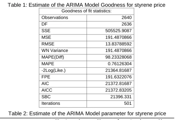
the ARIMA model was estimated. After several times trying, ARIMA (1,1,2) (0,0,0)

model was obtained to be the finest among the other family of ARIMA models. ARIMA Model goodness and parameters are given in Table 1 and Table 2.

Table 1: Estimate of the ARIMA Model Goodness for styrene price Goodness of fit statistics:

Observations 2640 DF 2636 SSE 505525.9087 MSE 191.4870866 RMSE 13.83788592 WN Variance 191.4870866 MAPE(Diff) 98.23328068 MAPE 0.76126304 -2Log(Like.) 21364.81687 FPE 191.6322076 AIC 21372.81687 AICC 21372.83205 SBC 21396.331 Iterations 501

Table 2: Estimate of the ARIMA Model parameter for styrene price

This model satisfies the inevitability condition and stationary condition and all the coefficients were found to be statistically significant at the 1% level of significance. As well as value, RMSE and MSE are 0.932, 10.837, 117.440 correspondingly at the model fitting stage. The appropriateness of the model was also adjudicated through the values of Box-Pierce Q statistics (17660.656 i.e.) it found to be unimportant. Thus, generally, we could say ARIMA (1,1,2) (0,0,0) model shown the acceptable result, among other ARIMA models.

The information about the Neural network structure indicates that network has an input layer with one input nodes, two hidden layers with 10,7 hidden nodes and an output layer with one output node means (1,10,7,1) feedforward network. The activation function is Sigmoidal at the hidden layer and the output layer. The error is the total sum of squares error because identity, activation function is used to the

Parameter Value Hessian standard error Lower bound (95%) Upper bound (95%) Asympt. standard error Lower bound (95%) Upper bound (95%) AR(1) 0.652 0.171 0.316 0.987 0.049 0.555 0.748 MA(1) -0.410 0.177 -0.757 -0.063 0.059 -0.526 -0.295 MA(2) -0.028 0.060 -0.146 0.090 0.019 -0.066 0.010

(13)

927

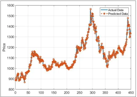
output layer. Figure 5 represents the Actual v/s ANN fitted plot of styrene price time

series.

Figure 5: Actual V/S ANN Fitted Plot of Styrene Price Time Series

In the next step, residuals are obtained from the fitted ARIMA model. Figure 6 reveals the ARIMA residuals plot of styrene price time series. The Dickey-Fuller test and Phillips-Peron test were applied to test the presence of non-linearity. The results of this test are brought in Table 3 that p-value is greater than the significance level alpha=0.05, which show that the nonlinear pattern is existent.

Figure 6: ARIMA Residuals Plot of Price Time Series

Table 3: Non-Linearity Testing For ARIMA of Styrene Price Time Series Phillips-Peron Dickey-Fuller

Tau (Observed value) -0.118 -2.956 Tau (Critical value) -1.941 -3.384 p-value (one-tailed) 0.643 0.142

(14)

928

ANN model specification for ARIMA residuals of styrene price time series

shows that network has an input layer with one input nodes, two hidden layers with 10,7 hidden nodes and an output layer with one output node means (1,10,7,1) feedforward network. The activation function applied is Sigmoidal at the hidden layer and the output layer. The error is the sum of squares error because identity, the activation function is applied to the output layer. Figure 7 represents ANN plot of residuals of styrene price time series.

Figure 7: ANN plot of residuals of styrene price time series

Forecasting performance of different models for styrene price time series in training dataset as given in Table 4, shows minimum MAPE, MSE, and RMSE value.

Table 4: Forecasting performance of different models for styrene price time series in training dataset

Criteria ARIMA ANN ARIMA-ANN

MSE 117.440 18.062 16.523

RMSE 10.837 4.253 4.012

MAPE 8.761 6.947 4.112

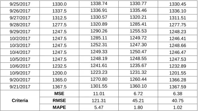
To calculate the forecasting performance last 14 observations of the considered time series was forecasted employing the offered approach. This approach was compared with the conventional ARIMA and Zhang hybrid approach (ARIMA-ANN). The results are given in the following Table 5 as a test set.

Table 5: Forecasting performance of different models for styrene price time series in testing data set

Date Actual Forecast

ARIMA ANN ARIMA-ANN

9/20/2017 1365.0 1361.77 1367.98 1365.22 9/21/2017 1367.5 1359.25 1369.21 1367.86 9/22/2017 1332.5 1345.29 1335.47 1331.12

(15)

929

9/25/2017 1330.0 1338.74 1330.77 1330.45 9/26/2017 1337.5 1336.91 1335.46 1336.10 9/27/2017 1312.5 1330.57 1320.21 1311.51 9/28/2017 1277.5 1320.89 1285.41 1277.75 9/29/2017 1247.5 1290.26 1255.53 1248.23 10/2/2017 1247.5 1285.11 1249.72 1246.41 10/3/2017 1247.5 1252.31 1247.30 1248.66 10/4/2017 1247.5 1249.33 1250.47 1246.47 10/5/2017 1247.5 1248.19 1248.55 1247.53 10/6/2017 1232.5 1241.61 1235.67 1232.89 10/9/2017 1200.0 1223.23 1231.32 1201.55 9/20/2017 1365.0 1270.80 1260.44 1366.28 9/21/2017 1367.5 1301.55 1360.10 1367.59 Criteria MSE 11.01 6.72 6.38 RMSE 121.31 45.21 40.75 MAPE 5.47 1.80 1.02

The comparative outcomes for the best ARIMA, ANN and ARIMA-ANN models are given in the Table 5. MSE, RMSE and MAPE statistic gives the indication of overall the superiority of ARIMA-ANN for forecasting of styrene price. Figure 8 represents the Actual v/s ARIMA-ANN fitted plot of styrene price time series.

Figure 8: Actual v/s ARIMA-ANN fitted plot of Styrene price time series

5. CONCLUSION

The price of styrene is important for the companies that produce styrene, as well as the companies, use it as a raw material. Hence, insight into likely future

(16)

930

behaviour and patterns of styrene prices can help decrease the impacts of styrene

price movements and unpredicted market fluctuations. One of the advantages of price forecasting is to efficiently manage the resources of an organization so that the organization can maximize the potential of the products or services produced or offered by the company.

The price of the styrene mostly depends on the financial steadiness of the company, turn over value, share volume and other variety of other financial and economic factors. Therefore, find the proper forecasting method to predict long/short-term price predictions is a large challenge today.

The traditional linear time series models are not always suitable for time series that have both linear and non-linear structures. As a result, this study generally concentrated attempted to recognizing the suitable hybrid forecasting approach based on ANN and ARIMA. The other purpose of predicting the future styrene price is because this predicted value can be used for future planning. Furthermore, model accuracy testing results of the mean absolute percentage error (MAPE) and (MAPE [ARIMA (1, 1, 2)] < MAPE [ANN], MAPE [ ARIMA (1, 1, 2)] < MAPE [ANN]), proposed that new hybrid method which combines linear and non-linear models can be proper way to improve forecasting performance.

Lastly, we toughly believed that the present study makes the important contribution to the manufacturer of styrene. Achievements of this study also will lead to all the styrene market role players in Iran. Furthermore, to provide protection for the organization against the occurrence of negatively-valence events while allowing the organization to benefit from the occurrence of positively-valence events.

There are certain limitations in forecasting. It becomes difficult to capture the exact change in case of a sudden change in the data set (when the variation is large) and in case of the change in economic instability in the world. Also, some forecasting methods might use the similar data but provide broadly different forecasts.

In further studies, one can improve the forecasting accurateness by using some other methods like machine learning techniques. It is recommended that the proposed method is applied to different markets/different products and the results shall be compared.

(17)

931

REFERENCES

AHMAD, H. A.; DOZIER, G. V.;. ROLAND, D. A. (2001) Egg price forecasting using neural networks. Journal of Applied Poultry Research, v. 10, p. 162-171. DOI: 10.1093/japr/10.2.162

AHMAD, W. K. A.; AHMAD, S. (2013) Arima Model and Exponential Smoothing Method: A Comparison. AIP Conference Proceedings, DOI: 10.1063/1.4801282 AS' AD, M. (2012) Finding the best ARIMA model to forecast daily peak electricity demand. Proceedings of the Fifth Annual ASEARC Conference - Looking to the future - Programme and Proceedings, 2 - 3 February, University of Wollongong. BARI, S. H.; RAHMAN, M. T.; HUSSAIN, M. M.; RAY, S. (2015) Forecasting monthly precipitation in Sylhet city using ARIMA model. Civil and Environmental Research, v. 7, n. 1, p. 69-77.

CHAKRAVARTY, A. (2016) Cognitive Routing - putting neurons in router.

Available at: https://www.linkedin.com/pulse/cognitive-routing-putting-neurons-router-amitabha-chakravarty/

CIECIERSKA, E.; BOCZKOWKA, A.; KUBIŚ, M.; CHABERA, P.; WIŚNIEWSKI, T. (2015) Effect of styrene addition on thermal properties of epoxy resin doped with carbon nanotubes. Polymers for Advanced Technologies, v. 26, n. 12, p. 1593-1599. DOI: 10.1002/pat.3586.

DAREKAR, A. S.; POKHARKAR, V. G.; DATARKAR, S. B. (2016) Onion Price Forecasting In Kolhapur Market of Western Maharashtra Using ARIMA Technique.

International Journal of Information Research and Review, v. 3, n. 12, p. 3364-3368.

DENTON, J. W. (1995) How good are neural networks for causal forecasting?. The Journal of Business Forecasting, v. 14, n. 2, p. 17.

ENERGY, U. D. O. (2013) wiki/Styrene#cite_note-DOE2010-5. [Online] Available at: http://www.enare,wikipedia.org.

GHAFFARI, A.; ZARE. S. (2009) A novel algorithm for prediction of crude oil price variation based on soft computing. Energy Economics, v. 31, n. 4, p. 531-536. DOI: 10.1016/j.eneco.2009.01.006.

GODARZI, A. A.; AMIRI, R. M.; TALAEI, A.; JAMASB, T. (2014) Predicting oil price movements: A dynamic Artificial Neural Network approach. Energy Policy, v. 68, p. 371-382. DOI: 10.1016/j.enpol.2013.12.049.

HAMID, S. A. (2004) Primer On using Neural Networks for Forecasting Market Variables. Southern New Hamshire University, s.n.

ICIS (2015) Styrene US Margin Report, London: Reed Business Information. JAIN, G.;. MALLICK, B. (2017) A study of time series models ARIMA and ETS.

Modern Education and Computer Science, v. 4, p. 57-63. DOI: 10.2139/ssrn.2898968.

KHASHEI, M.; BIJARI, M. (2011) A novel hybridization of artificial neural networks and ARIMA models for time series forecasting. Applied Soft Computing, v. 11, n. 2, p. 2664-2675. DOI: 10.1016/j.asoc.2010.10.015.

(18)

932

Research, v. 28, n. 4, p. 965-977. DOI: 10.1016/S0160-7383(01)00006-8. MADDEN, G.; TAN, J. (2007) Forecasting Telecommunications Data with Linear Models. Telecommunications Policy, v. 31, n. 1, p. 31-44.

MIYASHITA, K. (2012) Ethyl Benzene (EB) & Styrene Monomer (SM).Toyo Engineering Korea Ltd. Available at:

http://www.toyo-eng.com/kr/en/business/petrochemical/eb_sm/

MOMBEINI, H.; YAZDANI-CHAMZINI, A. (2015) Modeling gold price via artificial neural network. Journal of Economics, business and Management, v. 3, n. 7, p. 699-703.

MOVAGHARNEJAD, K.; MEHDIZADEH, B.; BANIHASHEMI, M.; KORDKHEILI, M. S. (2011) Forecasting the differences between various commercial oil prices in the Persian Gulf region by neural network. Energy, v. 36, n. 7, p. 3979-3984.

NAVEENA, K.; SUBEDAR, S.; SANTOSHA, R.; ABHISHEK, S. (2017) Hybrid time series modelling for forecasting the price of washed coffee (Arabica Plantation Coffee) in India. International Journal of Agriculture Sciences, v. 9, n. 10, p. 4004-4007.

NEWAZ, M. K. (2008) Comparing the Performance of Time Series Models for Forecasting Exchange Rate. BRAC University, p. 55-65.

OZOZEN, A.; KAYAKUTLU, G.; KETTERER, M.; KAYALICA, O. (2016) A combined seasonal ARIMA and ANN model for improved results in electricity spot price

forecasting: Case study in Turkey. 2016 Portland International Conference on Management of Engineering and Technology (PICMET). DOI:

10.1109/PICMET.2016.7806831.

PANELLA, M.; BARCELLONA, F.; D’ECCLESIA, R. L. (2012) Forecasting energy commodity prices using neural networks. Advances in Decision Sciences, v. 2012. DOI: 10.1155/2012/289810.

PAO, H. T. (2007) Forecasting electricity market pricing using artificial neural networks. Energy Conversion and Management, v. 48, n. 3, p. 907-912. RATHNAYAKA, R. M. K. T.; SENEVIRATNA, D. M. K. N.; JIANGUO, W.;

ARUMAWADU, H. I. (2015) A hybrid statistical approach for stock market forecasting based on Artificial Neural Network and ARIMA time series models. 2015

International Conference on Behavioral, Economic and Socio-cultural Computing (BESC). DOI: 10.1109/BESC.2015.7365958.

RUSIMAN, M. S.; HAU, O. C.; ABDULLAH, A. W.; SUFAHANI, S. F.; AZMI, N. A. (2017) An Analysis of Time Series for the Prediction of Barramundi (Ikan Siakap) Price in Malaysia. Far East Journal of Mathematical Sciences, v. 102, n. 9, p. 2081-2093.

SHABRI, A.; SAMSUDIN, R. (2014) Daily crude oil price forecasting using

hybridizing wavelet and artificial neural network model. Mathematical Problems in Engineering, v. 2014. DOI: 10.1155/2014/201402.

SHERMAN, L. M. (2010) Resin Prices Mostly Flat or Soft. Plastics Technology,

Plastics Technology Magazine, v. 56, n. 11, p. 37-38.

TULARAM, G. A.; SAEED, T. (2016) Oil-price forecasting based on various

(19)

933

3, p. 226-235.

VEIGA, C. P.; VEIGA, C. R. P.; CATAPAN, A.; TORTATO, U.; SILVA, W. V. (2014) Demand Forecasting in Food Retail: A Comparison between the Holt-Winters and ARIMA Models. WSEAS Transactions on Business and Economics, v. 11, p. 608-614.

YADAV, A.; SAHU, K. (2017) Wind forecasting using artificial neural networks: a survey and taxonomy. International Journal of Research In Science &

Engineering, v. 3, n. 2, p. 148-155.

YOUSEFI, M.; HOOSHYAR, D.; YOUSEFI, M.; KHAKSAR. W.; SAHARI, K. S. M.; ALNAIMI, F. B. I. (2015) An artificial neural network hybrid with wavelet transform for short-term wind speed forecasting: A preliminary case study. 2015 International Conference on Science in Information Technology (ICSITech). DOI:

10.1109/ICSITech.2015.7407784.

YOUSIF, E.; HADDAD, R. (2013) Photodegradation and photostabilization of polymers, especially polystyrene. SpringerPlus, v. 2, n. 1, p. 398.

YU, L.; WANG, S.; LAI, K. K. (2008) Forecasting crude oil price with an EMD-based neural network ensemble learning paradigm. Energy Economics, v. 30, n. 5, p. 2623-2635.

ZHANG, G. P. (2003) Time series forecasting using a hybrid ARIMA and neural network model. Neurocomputing, v. 50, p. 159-175.