From the Unit of Biostatistics, Institute of Environmental Medicine, Karolinska Institutet, Stockholm, Sweden
MATHEMATICAL PROGRAMMING FOR OPTIMAL
PROBABILITY WEIGHTING
Michele Santacatterina
All published papers reproduced with permission Published by Karolinska Institutet
Printed by E-Print AB 2018
Typeset by the author using LATEX 2ε ©Michele Santacatterina 2018
MATHEMATICAL PROGRAMMING FOR OPTIMAL PROBABILITY
WEIGHTING
THESIS FOR DOCTORAL DEGREE (Ph.D.)
By
Michele Santacatterina
Principal supervisor: Professor Matteo Bottai Karolinska Institutet
Institute of Environmental Medicine
Co-supervisors:
Professor Rino Bellocco University of Milano-Bicocca Department of Statistics and Quantitative Methods Professor Anna Mia Ekstr¨om Karolinska Institutet
Department of Public Health Sciences
Professor Anders Sonnerb¨org Karolinska Institutet
Department of Medicine
Opponent:
Assistant Professor Jos´e Ramon Zubizarreta Harvard University
Department of Health Care Policy
Examination board: Professor Timo Koski
Royal Institute of Technology Department of Mathematics Senior Lecturer Mark Clements Karolinska Institutet
Department of Medical Epidemiology and Biostatistics
Associate Professor Anna Grimby Ekman University of Gothenburg
Department of Public Health and Community Medicine
Abstract
In spite of the fact that probability weighting is widely used in statistics to correct for unequal sampling, control for confounding, and handle missing data, it has two main limita-tions. First, statistical inferences may be inefficient in the presence of extreme probability weights. Second, probability weighting-based methods are highly sensitive to model mis-specifications. The aim of this Ph.D. thesis work was to develop novel methods, based on mathematical programming techniques, for optimal probability weighting. Specifically, in Paper I, we proposed a method that estimates optimal probability weights, which are obtained as the solution to a constrained optimization problem that minimizes the Eu-clidean distance from the target (original/design) weights among all sets of weights that satisfy a constraint on the precision of the resulting weighted estimator. In Paper II, we extended optimal probability weights to estimate the causal effect of a time-varying treat-ment on a survival outcome. Optimal probability weights were obtained as the solution to a constrained optimization problem which constrained the variance of the weights, rather than the standard error of the resulting weighted estimator, as in Paper I. In Paper III, we proposed Kernel Optimal Weighting (KOW), to obtain weights that optimally balance time-dependent confounders while controlling for the precision of the resulting marginal structural model estimate by directly minimizing the error in estimation. This error is expressed as an operator derived from the g-computation formula and KOW minimizes its operator norm with respect to a reproducing kernel Hilbert spaces by solving a quadratic optimization problem. KOW mitigates the effects of possible misspecification of the treat-ment model by directly balancing covariates and control for precision by penalizing extreme weights. In Paper IV, we evaluated the effect of treatment switch on time to second-line HIV treatment failure using data from the Swedish InfCare HIV registry. This Ph.D. thesis provided methods that will likely help to (1) extend the use of probability weighting in medicine, epidemiology, and economics, (2) extend knowledge on how mathematical pro-gramming and machine learning could be used to conduct robust analyses for improved decision-making, and, (3) provide powerful, strong, and robust results to clinicians and policy-makers.
List of publications
I. Michele Santacatterina, and Matteo Bottai
Optimal probability weights for inference with constrained precision
Journal of the American Statistical Association 2017; in press
II. Michele Santacatterina, Rino Bellocco, Anders S¨onnerborg, Anna Mia Ekstr¨om, and Matteo Bottai
Optimal probability weights for estimating causal effects of time-varying treatments with marginal structural Cox models
Submitted 2018;
III. Michele Santacatterina, and Nathan Kallus
Optimal balancing of time-dependent confounders for marginal structural models
Manuscript 2018;
IV. Amanda H¨aggblom, Michele Santacatterina, Ujjwal Neogi, Magnus Gisslen, Bo Hejde-man, Leo Flamholc, and Anders S¨onnerborg
Effect of therapy switch on time to second-line antiretroviral treatment failure in HIV-infected patients
PloS one 2017; 12(7):e0180140
The articles will be referred to in the text by their Roman numerals, and are reproduced in full at the end of the thesis.
Other publications
Michele Santacatterina, and Matteo Bottai
Inferences and conjectures in clinical trials: a systematic review of gener-alizability of study findings
Journal of internal medicine 2016; 276(1):123–126
Niklas Karlsson, Michele Santacatterina, Kerstin K¨all, Maria H¨agerstrand, Susanne Wallin, Torsten Berglund, and Anna Mia Ekstr¨om
Risk behaviour determinants among people who inject drugs in Stock-holm, Sweden over a 10-year period, from 2002 to 2012
Contents
1 Introduction 1
2 Background 3
2.1 Weighting in survey sampling . . . 3
2.1.1 Calibration Estimators . . . 3
2.2 Missing data . . . 4
2.3 Causal Inference . . . 5
2.3.1 Inverse probability of treatment weighting . . . 6
2.3.2 Matching . . . 7
2.3.3 Covariate balancing . . . 8
2.3.4 Causal inference in longitudinal studies . . . 8
2.4 Limitations of probability weighting methods . . . 10
2.4.1 Extreme probability weights . . . 10
2.4.2 Model misspecification . . . 10
2.5 Kernels and Gaussian processes . . . 11
2.5.1 Kernels and reproducing kernel Hilbert spaces . . . 11
2.5.2 Gaussian processes for machine learning . . . 11
2.6 Mathematical Programming . . . 12
3 Aims of the thesis 13 4 Summary of the studies 14 4.1 Paper I . . . 14 4.1.1 Additional results . . . 15 4.2 Paper II . . . 15 4.3 Paper III . . . 20 4.4 Paper IV . . . 21 4.4.1 Additional results . . . 21 5 Discussion 23 6 Future research 24
References 27
Chapter 1
Introduction
Probability weighting is widely used in statistics to (1) correct for unequal sampling fractions, i.e. sampling weighting (Pfeffermann, 1993); (2) estimate the causal effect of a treatment (or intervention) from observational studies, i.e. inverse probability of treatment weighting (Robins et al., 1994); (3) handle missing data (Little and Rubin, 2014) and (4) generalize the study results from randomized trials (Stuart et al., 2011a).
The key idea of probability weighting is to correct for sample’s disproportionalities with respect to a target population of interest by weighting each unit in the sample. For example, when estimating the causal effect of a treatment on an outcome with observational data, the target population of interest is that in which covariates are balanced across treatment groups. Each unit is consequently weighted by the inverse of the probability of being assigned to the treatment conditional on covariates.
It is well known, however, that statistical inference may be inefficient when weights contain outlying values (Rao, 1966; Basu, 2011; Robins et al., 2007, 1995; Scharfstein et al., 1999, among others). In addition, in the context of causal inference, inverse probability of treatment weighting methods are highly sensitive to misspecifications of the treatment model (Kang and Schafer, 2007b; Lefebvre et al., 2008; Cole and Hern´an, 2008).
Mathematical programming, also know as optimization, is a branch of mathematics that concerns the theory and development of methods that find extrema of an objective function (Luenberger and Ye, 2015). Examples include running a business in which profit has to be maximized or losses minimized, and the selection of a flight route which minimizes the fuel cost. Mathematical programming is also used in the context of probability weighting. For example, calibration estimators in survey sampling use calibration weights which are obtained by solving a constrained optimization problem (Deville and S¨arndal, 1992). Optimal matching, used to balance covariates in observational studies, can be reinterpreted as a network flow optimization problem (Rosenbaum, 1989).
In this Ph.D. thesis, we present methods, based on mathematical programming tech-niques, that (1) provide a set of weights, called optimal probability weights, which are the closest to the target (original/design) weights of interest while controlling the precision of the resulting weighted estimator; (2) extend optimal probability weights to the estimation
2 1. Introduction
of the causal effect of a time-varying treatment on a survival outcome; and (3) provide weights that optimally balance time-dependent confounders, thus mitigating the effects of possible misspecification of the treatment model, and control for the precision of the resulting marginal structural model estimate. We apply the proposed methods to the study of the effect of timing of treatment initiation on long-term treatment efficacy in patients infected with human immunodeficiency virus (HIV).
A motivational example
This Ph.D. work was motivated by the abundant use of probability weighting in observa-tional studies to estimate the effect of treatment initiation among people who live with HIV (Hern´an et al., 2000, 2001; HIV-Causal Collaboration et al., 2010, 2011; Lodi et al., 2017, among others). For example, Cole and Hern´an (2008) evaluated the effect of HIV treatment initiation on the evolution of CD4 cell count by estimating the parameters of the marginal structural model using inverse probability of treatment weighting. Weights were obtained as the inverse of the probability of treatment initiation given a set of baseline covariates. The authors concluded that the effect of HIV treatment initiation on differences in CD4 cell count after one year of treatment was equal to 29 with a 95% confidence interval (CI) equal to (15.8;42.3). The unweighted analysis reported an effect equal to -6 with a 95% CI equal to (-4.4;3.1). The weighted estimate was highly variable, with a confidence interval almost four times that of the unweighted estimate. To control for extreme weights, the authors truncated the weights by replacing outlying values with smaller ones. A new estimate of the effect of HIV treatment was obtained (25; 95% CI (11.6;38.9)). The authors further suggested to model the treatment assignment in a flexible way, e.g. including splines, to control for model misspecification.
Chapter 2
Background
2.1
Weighting in survey sampling
The general goal of weighting in survey sampling is to find a set of weights that corrects for disproportions in the sample, thus making the sample representative of a target population of interest. We may be interested in estimating a parameter, such as the mean, of this target population. To provide an example on how weighting is used, let us consider sampling two samples of sizesn1 andn2 from two strata,S1 andS2 of known sizesN1 andN2. Suppose we are interested in estimating the population totaltY. A natural estimator for tY is the
sample mean weighted by each population total, i.e. ˆtY =N1y¯1+N2y¯2. This expression can also be written as,
ˆ tY =N1 X i∈S1 yi n1 +N2 X i∈S2 yi n2 (2.1) = X i∈S1 yi n1/N1 +X i∈S2 yi n2/N2 (2.2) =X i yi πi (2.3)
whereπi=nj/Nj ifi∈Sj and j∈1,2 are the inclusion probabilities. By weighting each
sampledyi for the inverse of its probability of selection, we obtain an unbiased estimate
of the population total. The estimator ˆtY is called the Horvitz-Thompson (HT) estimator
(Horvitz and Thompson, 1952). In this thesis, we refer toY as a random variable, to y as its realization, and toE[Y] as the expected value of Y.
2.1.1 Calibration Estimators
Auxiliary information about the target population, such as population means or totals, obtained from sources different than the survey, such as census, is widely used in survey sampling to improve survey estimates (Foreman and Brewer, 1971; Deville and S¨arndal, 1992; Valliant et al., 2013). For example, Deville and S¨arndal (1992) proposed a family
4 2. Background
of calibration estimators in which auxiliary information is incorporated. These estimators use calibrated weights, defined as the closest weights, given a distance measure, to the original sampling design weights that satisfy a set of constraints called calibration equations. Specifically, let us consider a sampleS selected from a finite population U and consider the sampling design weightsdi = 1/πi ∀ i∈S, and the HT estimator, ˆtY =Pi∈Syi/πi = P
i∈Sdiiyi. Let us further assume that we have auxiliary information in the form of the
population total ofX,tX =P
i∈Uxi, wherexi = (xi1, . . . , xip)T is the observed vector ofp
auxiliary variables. A calibration estimator is the estimator, ˆtcY =P
i∈Swiyi, with weights
wi, ∀i∈S which minimize a measure of distance,L(w, d) while satisfying the following
calibrating equation,
X
i∈S
wixi=tX. (2.4)
One choice of distance L(w, d) is the least-squares distance function P
i∈S(wi−di)2/di.
Minimization leads to the calibrated weights,
wi=di(1 +xTi λ), (2.5)
where λ is the vector of Lagrange multipliers determined from (2.4) and equal to λ = (XTDX)−1(tX−tˆX). The resulting estimator of tY is
ˆty = ˆtY + (tX−ˆtX)TBˆ, (2.6)
where ˆB = (XTDX)−1XTDy is the solution to the weighted least square estimator, and ˆtX = XTD. Calibration estimators provide a different derivation of the generalized regression estimator (Cassel et al., 1976; S¨arndal, 1980) in which auxiliary information is included. In addition, calibration estimators provide an example of the use of mathematical programming to obtain weights that satisfy specific constraints. Lumley et al. (2011) showed a connection between calibration estimators and the augmented inverse probability weighting estimator for missing data and causal inference proposed by Robins et al. (1994).
2.2
Missing data
Weighting can also be used to control for missing data. By missing data, we mean data values that are unobserved. Examples include non-response in survey sampling, when randomly chosen individuals provide partial or no answer, and dropout/non-compliance in randomized clinical trials, where individuals initially randomized to one treatment, do not show up for any clinical visits or occasionally miss visits. Missing data leads to samples that are non-representative of the target population, thus introducing selection bias. We now provide an example on how weighting is employed to control for this type of bias. Consider a randomized trial, in which units are randomly assigned to a treatment or placebo. Specifically, letAi = 1 denotes the units assigned to the treatment, and Ai = 0
2. Background 5
those assigned to placebo, for all i= 1, . . . , n, wheren is the sample size. Let Yi be the
outcome under study. The parameter of interest is the average treatment effect (ATE), ∆ = µ1 −µ0, where µt, t ∈ {0,1} is the mean outcome among treated and placebo
individuals. Let us further definefull data, the data we would have liked to have collected,
observed data, the data actually observed, and complete data, the subset of the sample in which complete, non-missing, information is available. Having access to the full data, we would allow estimating ∆ with the unbiased estimator ˆ∆ = ˆµ1−µ0. Let us now denoteˆ by Ri, i = 1, . . . , n, the indicator of complete data, with Ri = 1 meaning that the i-th
measurement was taken, andRi = 0 meaning that it was missing. In this specific scenario,
we would observe (Ai, Ri, RiYi), i = 1, . . . , n. By focusing our attention on the treated
patients, i.e.Ai = 1, the observed data are denoted by (Ri, RiY1i),i= 1, . . . , n1, whereY1i
is thei-th observed outcome among the treated. Under the assumption that the data are missing completely at random (MCAR), i.e. the probability of being missing (or observed) does not depend onY1i1, the complete-case (CC) estimator ˆµ1CC =Pni=11 RiY1i/Pni=11 Ri
is an unbiased estimator for the ATE. When non-missing auxiliary information aboutp auxiliary variables, denoted byXi = (Xi1, . . . , Xip),i= 1, . . . , n is available, we can relax
the MCAR assumption, with that of missing at random (MAR), defined asRi ⊥⊥Yi1|Xi.
MAR means that the missingness mechanism is described in some way by the observed informationXi. Under MAR, weighting by the inverse of the probability of being a complete
case suggest the following inverse probability weighted complete case (IPWCC) estimator (Tsiatis, 2007; Robins et al., 1994),
ˆ µ1,IP W =n−11 n1 X n=1 riy1i π(xi) (2.7)
where π(Xi) = P(Ri = 1|Xi, Yi1) = P(Ri = 1|Xi)2 is the probability that the i-th
randomly selected individual with auxiliary informationXi, has complete data, and π(xi)
is its realization. The intuition behind the IPWCC estimator is that a sampled individual, with probability of having complete data equal to π(Xi), represents 1/π(Xi) individuals
from the population. Usually,π(Xi) is estimated from the data by using a logistic regression
or a classification algorithm (Lee et al., 2010; Friedman et al., 2001), and it must be bounded away from zero for all values ofXi. Similar assumptions and conditions are employed in
the literature of causal inference under the name of ignorability and positivity, respectively (Imbens and Rubin, 2015). More on inverse probability weighting and missing data can be
found in Seaman and White (2013).
2.3
Causal Inference
Most of the studies in science aim at answering causal rather than associational questions. For example, a medical doctor is interested in the effect of a treatment on some clinical
out-1
MCAR:Ri⊥⊥Yi1 andP(Ri= 1|Yi1) =π, for alli= 1, . . . , n.
2
6 2. Background
comes, while a policy maker is interested in the effect of a new policy compared with an old one. While randomized experiments provide unbiased estimates of the ATE, economic and ethical limitations make them not viable with only observational data available. Although potentially huge in sample size, these data sets are observational, where causal effects are hidden by confounding factors which must be controlled for. The following are some known methods to control for confounding and estimate causal effects with observational data. 2.3.1 Inverse probability of treatment weighting
Potential outcomes provide a framework in which causal effects can be estimated from observational data (Rosenbaum and Rubin, 1983). A potential outcomeY(a) is the outcome we would see if we were to be treated with treatmenta. Specifically, letT denote an indicator variable defining treatment allocation (A= 1 if treated, and A= 0 if control), and let X
be a vector of observed variables measured before treatmentA was assigned. LetY be the observed response variable formalized as
Y =Y(1)A+ (1−A)Y(0) (2.8) where the random variables Y(1) andY(0) respectively represent the potential outcomes of a treated and of an untreated individual. Let ∆ =E(Y(1)−Y(0)) =µ1−µ0 indicate the causal parameter of interest, the ATE, andµ1 andµ0 indicate the true means under each treatment. Under the assumption of
consistency: the observed outcome corresponds to the potential outcome of applying treatment a, i.e.Y =Y(a) ifA=a,
positivity3: the probability of getting treated given covariates is bounded away from zero and one, i.e. π(X) =P(A= 1|X),0< π(X)<1,
ignorability4: the potential outcome is independent to the treatment assignment mechanism given covariates, i.e. (Y(0), Y(1))⊥⊥A|X,
inverse probability of treatment weighting provides unbiased estimates of the ATE when using observational data. In particular, it can be shown that
ˆ ∆IP W =n−1 n X i=1 aiyi π(xi) − (1−ai)yi (1−π(xi)) =µ1−µ0 (2.9)
where π(xi) is the observed realization of the propensity score for the i-th individual.
Models, such as logistic regression, are used to estimate the unknown probabilityπ(xi). In
case these models are incorrect, i.e. misspecification of the treatment assignment model, the IPW-estimator in (2.9) is biased. Augmented inverse probability weighting estimators
3
also referred to as experimental treatment assignment or strict overlap 4
2. Background 7
(AIPW) (Scharfstein et al., 1999) have been proposed to overcome this issue. The key idea of AIPW is to combine regression and IPW estimators in one doubly robust (DR) estimator (Bang and Robins, 2005). DR refers to the fact that unbiased estimate of the ATE can be obtained whenever either of the outcome model or the propensity score model is correctly specified. Authors showed, however, that DR estimators may yield highly biased inferences when neither of the two models is correctly specified (Kang and Schafer, 2007a). Inverse probability weighting is also used to consistently estimate the parameters of a marginal structural model (MSM) (Robins, 2000). MSM are causal models in the form, for example, of E(Y(a)) =β0+β1a, where β1 is the causal parameter of interest. Weighted ordinary least square estimator is tipically used to estimateβ1. MSM have been extensively used to estimate the causal effect of a time-varying treatment on an outcome of interest, such as, for example, time to death (Robins et al., 1999; Robins, 2000; Hern´an et al., 2001). 2.3.2 Matching
Matching is a widely used technique to control for confounding in observational studies (Stuart et al., 2011b). The essential idea of matching is to assign one or more controls with similar observed covariates to each treated unit, thus balancing their distributions and, consequently, control for confounding. In the past decades, several matching methods have been developed, and the literature on the topic is vast (see Stuart et al. (2011b) for a review). Several measures of distance are used to evaluate if a control is a good match for a treated unit. Commonly used measures are
exact, Dij ={0, ifXi =Xj;∞, ifXi =Xj};
Mahalanobis, Dij = (Xi−Xj)TΣ−1(Xi−Xj), where Σ is the variance covariance
matrix in the full control group when estimating the average treatment effect on the treated (ATT) and that ofX in the full control and pooled treatment groups when estimating the ATE; and
Propensity score,Dij =|π(Xi)−π(Xj)|where π(Xi) is the propensity score for the
i-th individual.
“Greedy” and optimal matching methods are the most popular used matching algorithms. An example of a greedy matching method is the nearest neighbor matching method, in which a control individual, with the smallest distance from the treated, is selected for each treated individual. Rosenbaum (2002), showed how greedy methods can perform poorly as matching methods. In contrast, optimal matching (Rosenbaum, 1989), proposes to choose individual matches by minimizing a global measure of distance. This method is related to the literature of network flow theory, in which the standard problem is to find a flow of minimal cost in a network. In particular, Rosenbaum (1989) showed that optimal matching can be reinterpreted as a “personnel assignment” mathematical programming problem (Kuhn, 1955). Recently, Kallus (2016) proposed a class of generalized optimal matching methods,
8 2. Background
which includes many existing matching methods such as nearest-neighbor matching, optimal caliper matching, 1:1 matching, coarsened exact matching, and various near-fine balance approaches.
2.3.3 Covariate balancing
The ultimate goal of IPW and matching is to balance covariates in order to obtain an unbiased estimate of the causal parameter of interest. Methods that combine the spirit of probability weighting and matching have received recent attention. Kallus (2016) rein-terpreted optimal matching by providing balancing weights that balance covariates. Imai and Ratkovic (2014), proposed covariate balancing propensity score in which covariate balance is optimized. Hainmueller (2012) presented entropy balancing method, in which each observation is weighted to achieve optimal balance and the Kullback-Leibler diver-gence from a set of target weights is minimized. Chan et al. (2016) presented a general class of calibration estimators, which are constructed to attain exact three-way balance. Zubizarreta (2015) proposed a set of weights that are stabilized, i.e. have minimum variance while balancing covariates. Li et al. (2017) proposed a set of new weighting schemes which balance covariates via propensity ccore weighting. Athey et al. (2016) developed a method that allows sparse regression methods to be used to estimate ATE in high-dimensional linear models. Hirshberg and Wager (2017) proposed a method that efficiently estimates treatment effects by using weights that directly optimize worst-case risk bounds. Wong and Chan (2017) proposed a method that uniformly approximate covariate balance for functions in a reproducing-kernel Hilbert space. Zhao (2016) proposed to balance covariates by using tailored loss functions.
2.3.4 Causal inference in longitudinal studies
In longitudinal studies, where T measures are collected for each unit i = 1, . . . , n, the causal effect of a time-varying treatment on an outcome of interest can be estimated. Standard methods such as regression adjustment or matching fail to provide consistent estimate of the causal effect in presence of time-dependent confounders (Robins, 2000; Blackwell, 2013). Time-dependent confounders are time-varying factors that are affected by previous treatments and affect future ones (Robins, 2000). A common example of the role of time-dependent confounder is given by CD4 cell count in the study of the effect of HIV treatment on mortality among HIV-infected patients (Hern´an et al., 2000, 2001; HIV-Causal Collaboration et al., 2010, 2011; Lodi et al., 2017). CD4 cell count is both an independent predictor of initiation of HIV treatment and survival as well as being itself influenced by prior HIV treatment. Methods to deal with time-dependent confounding have been proposed in the statistical literature (Daniel et al., 2013). Among others, MSM have been used to estimate the causal effect of a time-dependent treatment on an outcome of interest. For eachaT, we define the MSM for the effect of a time-varying treatment on
2. Background 9
E[Y(aT)] =g(aT, β) (2.10)
where g(aT, β) is some known function, for example g(aT, β) = β1 + ∆PTt=1(at), the
parameter ∆ is the causal parameter of interest and Y(aT) is the potential outcome if
the unit were to be treated with treatment regimeaT. Under consistency, positivity and
sequential ignorability (Imbens and Rubin, 2015; Hernan and Robins, 2010), IPW is used to consistently estimate the parameters of the MSM. Inverse probability of treatment weights are defined as w(aT, xT) = T Y t=1 h(At) P(At=at|At−1 =at−1, Xt=xt) (2.11)
where At is the binary treatment variable at time t, Xt the time-dependent confounders
at timet, At is the treatment history up to time t, Xt is the history of time-dependent
confounders up to timet, andh(At) is a known function of the treatment history bounded
between zero and one. The set of inverse probability weights is obtained by settingh(At) =
1, while the set of stable inverse probability weights is obtained by settingh(At) =P(At=
at|At−1=at−1). Weights in the form of (2.11) are estimated by using parametric methods
such as logistic regression, along with other methods based on the literature of statistical learning (Karim et al., 2017; Gruber et al., 2015; Karim and Platt, 2017). Other methods such as g-computation formula (Robins, 1986), and g-estimation of structural nested models (Robins, 2000) provide alternative solutions to the problem of time-dependent confounders.
A review can be found in Daniel et al. (2013).
Matching for longitudinal data. Matching has also been used in the context of longitudinal data. Li et al. (2001) proposed optimal balanced risk set matching, in which a patient with similar history of symptoms up to time t is matched to a patient that receive treatment at timet. The method is based on the solution of a integer programming problem. Lu (2005) proposed a time-dependent propensity score used in risk set matching, which is based on the Cox proportional hazards model. It is not clear, however, if these methods can control for time-dependent confounding.
Covariate balancing for longitudinal data. Differently from inverse probability weights, Imai and Ratkovic (2015) proposed to estimate weights by generalizing the co-variate balancing propensity score (CBPS) methodology. CBPS estimates robust inverse probability weights for MSM by optimizing covariate balance. However, CBPS does not control for informative censoring.
10 2. Background
2.4
Limitations of probability weighting methods
As described in the previous sections, probability weighting methods are widely used in statistics. It is well known, however, that they have limitations. These limitations are: (1) statistical inference may be inefficient when weights contain extreme values; (2) statistical inference may be highly biased in case of model misspecifications.
2.4.1 Extreme probability weights
In today’s medical and epidemiological research, the most popular approach to deal with extreme weights is truncation, which consists of replacing outlying weights with smaller weights. For example, all weights above the 99th percentile of their sample distribution may be replaced with the 99th percentile itself. Methods have been proposed to obtain optimal cutoff points (Potter, 1990; Cox and McGrath, 1981; Kokic and Bell, 1994; Rivest et al., 1995; Hulliger, 1995). Approaches other than truncation, have been proposed (Pfeffermann and Sverchkov, 1999; Beaumont, 2008; Beaumont et al., 2013; Elliot and Little, 2000; Elliott, 2009; Zubizarreta, 2015). In longitudinal studies, truncation remains the only method used to control for extreme weights (Cole and Hern´an, 2008; Xiao et al., 2013).
2.4.2 Model misspecification
The propensity score needs to be estimated from the data. Several authors showed that in case of misspecification of the missing/treatment mechanism model, biased estimates of the parameter of interest are obtained. The problem is exacerbate in longitudinal study, where probability weights are multiplied across time points. Covariate balance methods, introduced in Section 2.3.3, mitigate the effect of possible model misspecification of the parametric model for the propensity score by obtaining weights that maximize the resulting covariate balance. To fix ideas, under consistency, positivity and ignorability and by the law of total probability (LTE), consider ∆ = E(Y(1)−Y(0)) the parameter of interest and consider the following decomposition based on the weighted average,
E[W1[A=a]Y] =E[W1[A=a]Y(a)] (by consistency) =E[WE[1[A=a]Y(a)|X]] (by LTE)
=E[WE[1[A=a]|X]E[Y(a)|X]] (byY(a)⊥⊥T|X) =E[E[Y(a)|X]] +δa
=E[Y(a)] +δa
(2.12)
whereE[1[A=a]|X] is the propensity score. One way to obtain an unbiased estimate of ∆ is to use inverse probability weights W = 1/E[1[A=a]|X]. A more robust5 way is to
5
2. Background 11
find a set of weights that makes δa = 0, a∈0,1 by balancing E[Y(a)|X] across treated
and controls.
2.5
Kernels and Gaussian processes
In this section we briefly introduce the concepts of kernels, reproducing kernel Hilbert spaces and Gaussian processes for machine learning.
2.5.1 Kernels and reproducing kernel Hilbert spaces
A kernel is a function that quantifies the similarities between observations and refers to a dot product between observed characteristics of the individual, referred to as features. Specifically, a functionk:X × X →Ris defined as a kernel if there exist a mapφ:X → H
and anR-Hilbert space such that∀x, x> ∈ X,
k(x, x>) :=Dφ(x), φ(x>)E
H. (2.13)
For a formal definition of Hilbert space and inner product see Sch¨olkopf and Smola (2002). All kernels are positive definite functions. Typical kernels are,
Linear kernel: k(x, x>) =x·x>.
Polynomial kernel: k(x, x>) = (x·x>+ 1)d, d∈N. Gaussian kernel: k(x, x>) =e−
kx−x>k2
σ2 , σ >0.
The space of functions defined by a kernel on the feature spaceX is known as reproducing kernel Hilbert spaces (RKHS). RKHS satisfy, among others, the reproducing property, ∀ x ∈ X,∀ f ∈ H, hf, k(·, x)iH = f(x), i.e. the evaluation of f at x can be interpreted as an inner product in feature spaces. RKHS are used in supervised learning, such as classification, in which the task is to choose where a new observation belongs between two or more categories, e.g. support vector machines (Sch¨olkopf and Smola, 2002). The key idea is to transform the data from the observed features spaceX into a higher dimensional space H, thus allowing to linearly separate the data. This idea refers to as the “kernel trick” (Hofmann et al., 2008).
2.5.2 Gaussian processes for machine learning
A Gaussian process (GP) is a stochastic process in which any finite finite number of random variables has a joint normal distribution (Rasmussen, 2004). A GP is completely specified by its mean and covariance function, defined as
m(x) =E[f(x)] k(x,x>) =E[(f(x)−m(x)) f(x>)−m(x>) ] (2.14)
12 2. Background
and it is usually defined asf(x)∼ GP m(x), k(x,x>). A GP can be viewed as a machine learning prediction algorithm. For example, the Bayesian linear regression modelf(x) = φ(x)Tβ with prior β∼ N(0,Σp),Σp =E[ββT] with mean and covariance
E[f(x)] =φ(x)TE[β] = 0 E[f(x)f(x0)] =φ(x)TΣpφ(x0)
(2.15) is a GP. Based on the results presented in Section 2.5.1, the covariance function can be obtained by using kernels. Different choices of the kernel are employed for different prediction problems, such as regression and classification. Once a kernel has been chosen, its hyperparameters, the parameters for which the covariance function depends on, are usually obtained by minimizing the log-likelihood with respect to those parameters. More on GP for machine learning can be found in Rasmussen (2004).
2.6
Mathematical Programming
In general terms, mathematical programming, also refereed to as optimization, is the task of minimizing a risk function with or without constraints (Griva et al., 2009). This topic covers minimization of one variable, convex minimization, maximization problems, constrained optimization, and non-convex optimization. Letpbe a vector of parameters inRk, a general
form of constrained optimization problem follows, minimize p∈Rk f(p) subject to gi(p)≤0, i∈ I, I ∪ε={1, . . . , m} hi(p) = 0, i∈ε, I ∩ε=∅ p≥0 (2.16)
where f : Rk 7→ R , g : Rk 7→ Rm and h : Rk 7→ Rn, and where p ≥ 0 are k bound
constraints. In this thesis we will mainly consider problems in the form of (2.16) with f(p) stricly convex and, when present,gi convex, thus admitting unique solution. Given
some regularity conditions, the Karush Kuhn Tucker (KKT) conditions are first-order necessary condition for a solution of problems in the form of (2.16). KKT generalizes the method of Lagrange multipliers to linear constraints. Apart of few special cases, in which analitical solutions can be found, the system of inequalities and equations obtained from the KKT conditions is solved by using optimization algorithms. Examples include, quadratic programming methods, which are used in Paper II and III and the primal-dual interior point method, which is used in Paper I. Algorithms are implemented in readily available software, such as theRpackagesGurobi and IPOPTR.
Chapter 3
Aims of the thesis
The overall aim of this thesis was to develop, investigate, and apply novel methods to estimate optimal probability weights.
More specifically, it aimed
to develop a method to estimate optimal probability weights that controls for the precision of the resulting weighted estimator;
to extend optimal probability weights when interested in the estimation of the causal effect of a time-varying treatment on a survival outcome;
to develop a novel method that simultaneously balances time-dependent confounders and control for the precision of the resulting marginal structural model estimate in longitudinal studies;
to show the applicability of the proposed methods by using data from the HIV literature.
Chapter 4
Summary of the studies
4.1
Paper I
The aim of Paper I was to develop a method to estimate optimal probability weights. Optimal probability weights are the solution to a constrained optimization problem that minimizes the Euclidean distance from the target (original/untruncated) weights among all sets of weights that satisfy a constraint on the precision of the resulting weighted estimator. Specifically, let ˆθw∗ be an unbiased estimator for a population parameter θ∗ that uses weightsw∗ = (w∗1, . . . , wn∗)T, with1Tw∗ = 1 andw∗ ≥0. The set ofw∗can be, for example, the set of inverse probability weights used to control for missing data or confounding. When w∗ contains outliers, the standard error σw∗ may be large and inference onθ∗ inefficient. We suggest deriving the weights ˆw that are closest to w∗ with respect to the Euclidean normkw−w∗k, under the constraint that the estimated standard error ˆσwˆ be less than or equal to a specified constantξ >0. The corresponding constrained optimization problem can be written as follows,
minimize w∈Rn kw−w ∗k 2 (4.1) subject to σˆw ≤ξ (4.2) w≤ (4.3) w≥0. (4.4)
Constraint (4.9) guarantees that the estimated standard error of the estimator with weights ˆ
wis less than or equal toξ. Constraints (4.10) and (4.11) guarantee that the optimal weights ˆ
ware bounded and non-negative, respectively. In Section 3 of Paper I, we described how the Lagrange multipliers and objective function from the optimization problem can help assess the trade-off between bias and precision of the weighted estimator. In a simulation study, we showed that optimal probability weights performed better than truncated weights with respect to bias and mean squared error of weighted least-squares regression coefficients. We also showed that optimal probability weights often led to large gains in precision at
4. Summary of the studies 15
the cost of small bias. We illustrated the use of optimal probability weights in an analysis of the effect of timing of treatment initiation on long-term health outcome in patients infected by HIV, using data from the Swedish InfCare HIV registry. Our findings indicated that the age at the start of treatment was a relevant effect modifier, and correct timing of treatment initiation was more important in younger patients.
4.1.1 Additional results
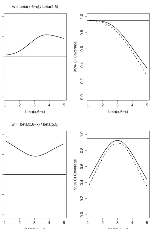
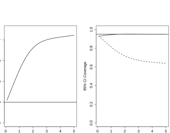
In addition to the results provided in Paper I, we also constructed 95% confidence intervals for all the scenarios reported in Figures 1 and 2 of Paper I. The observed coverage is shown in Figures 4.1-4.4 below. In all scenarios, when the optimal weights are close to the target weights, the bias of the optimal estimator, ˆθwˆ, with respect to the target parameter,θw∗, is slight and the observed coverage of the confidence interval is near the nominal level. As the optimal weights move away from the target weights, the bias increases and the coverage decreases. The coverage of the truncated estimator, ˆθw¯, is always worse than that of the optimal estimator, ˆθwˆ, especially in the presence of a strong confounding effect (Figure 4.3).
4.2
Paper II
The aim of Paper II was to extend optimal probability weights to estimating the causal effect of a time-varying treatment on a survival outcome. As shown by Hern´an et al. (2001), inverse probability of treatment and censoring weighting is used to consistently
estimate the parameters of the marginal structural Cox model. However, these methods rely substantially on the positivity assumption. Practical violations of the positivity assumption are common with survival data, resulting in extreme weights, low precision and erroneous inferences. As presented in Paper I, truncation is the most used technique to control for extreme weights. In Paper II, we proposed to obtain weights ˆw(ot)that are the closest to ˆw(∗t),
the estimated set of target (original/untruncated) weights, with respect to the Euclidean norm, while constraining the variance of the weights ˆwo(t) to be less or equal to a specified
levelξ. The resulting quadratic optimization problem can be formulated as follows,
minimize
w(ot)∈Rn×t
kw(ot)−wˆ∗(t)k2 (4.5) subject to kw(ot)−wo(t)k22 ≤ξ (4.6)
w(ot)≥0 (4.7)
where w(ot) is the mean of the weightsw(ot). Differently from Paper I, where we constrained
the standard error of the resulting weighted estimator, in Paper II we constrained the variance of the weights. This formulation of the optimization problem is novel and has two main advantages: (1) it is quadratic and convex and therefore admits a unique solution; and (2) it is independent of both the chosen estimator for the causal parameter of interest
16 4. Summary of the studies 1 2 3 4 5 0.0 0.5 1.0 1.5 2.0 w = beta(x,6−x) / beta(2,5) beta(x,6−x) MSE r atios 1 2 3 4 5 0.0 0.2 0.4 0.6 0.8 1.0 beta(x,6−x) 95% CI Co v er age 1 2 3 4 5 0.0 0.5 1.0 1.5 2.0 w = beta(x,6−x) / beta(5,5) beta(x,6−x) MSE r atios 1 2 3 4 5 0.0 0.2 0.4 0.6 0.8 1.0 beta(x,6−x) 95% CI Co v er age
Figure 4.1: The right-hand-side panels show the observed coverage of 95% confidence intervals using optimal weights (solid lines) and truncated weights (dotted) corresponding to the scenarios considered in the left-hand-side panels of Figure 1 of the manuscript, which are reported in the left-hand-side panels above.
4. Summary of the studies 17 0.5 0.6 0.7 0.8 0.9 1.0 0.0 0.1 0.2 0.3 0.4 Proportion of σ^w 2 0.5 0.6 0.7 0.8 0.9 1.0 0.0 0.2 0.4 0.6 0.8 1.0 beta(x,6−x) 95% CI Co v er age 0.5 0.6 0.7 0.8 0.9 1.0 0.0 0.1 0.2 0.3 0.4 Proportion of σ^w2 0.5 0.6 0.7 0.8 0.9 1.0 0.0 0.2 0.4 0.6 0.8 1.0 beta(x,6−x) 95% CI Co v er age
Figure 4.2: Observed coverage of 95% confidence intervals (right-hand-side panels) corresponding to the scenarios considered in the right-hand-side panels of Figure 1 of the manuscript, which are reported in the left-hand-side panels above.
18 4. Summary of the studies 0 1 2 3 4 5 0 1 2 3 4 Effect of covariate C MSE r atios 0 1 2 3 4 5 0.0 0.2 0.4 0.6 0.8 1.0 Effect of covariate C 95% CI Co v er age
Figure 4.3: The right-hand-side panel shows the observed coverage of 95% confidence intervals using optimal weights (solid lines) and truncated weights (dotted) corresponding to the scenarios considered in the left-hand-side panel of Figure 2 of the manuscript, which is reported in the left-hand-side panel above.
4. Summary of the studies 19 0.5 0.6 0.7 0.8 0.9 1.0 0.0 0.2 0.4 0.6 0.8 Proportion of σ^w2 0.5 0.6 0.7 0.8 0.9 1.0 0.0 0.2 0.4 0.6 0.8 1.0 Proportion of σ^w2 95% CI Co v er age
Figure 4.4: Observed coverage of 95% confidence intervals (right-hand-side panel) corresponding to the scenarios considered in the right-hand-side panel of Figure 2 of the manuscript, which are reported in the left-hand-side panel above.
20 4. Summary of the studies
and that for its standard error. The optimization problem in (4.8), can be reformulated as a unconstrained problem in which we shrink/penalize the variance of the weights by a penalization parameter λ. In a simulation study we showed how the bias and mean square error of the causal effect of a time-varying treatment that used the proposed weights outperformed the truncated weights across all the considered truncation levels, especially at high percentiles. We illustrated the use of the proposed weights to evaluate the causal effect of treatment initiation on time to death among people who live with HIV, using data from the Swedish InfCare HIV registry. We concluded that people who live with HIV can benefit from being treated.
4.3
Paper III
The aim of Paper III was to develop a novel method that provides weights that optimally balance time-dependent confounders while controlling for the precision of the resulting MSM estimate. Specifically, MSM have been widely used to estimate the causal effect of a time-varying treatment on an outcome in the presence of time-dependent confounding. These methods, however, have two main limitations: (1) as shown in Paper I and II, they heavily rely on the positivity assumption, and (2) they are highly sensitive to the misspecifiation of the treatment assignment model. Various statistical methods have been proposed in an attempt to overcome these challenges. To control for misspecification of the treatment assignment model, Imai and Ratkovic (2015) proposed covariate balance propensity score (CBPS), which estimates robust inverse probability weights for MSM by optimizing covariate balance. The method ensures that the first moment of each covariate is balanced even in case of model misspecification (Imai and Ratkovic, 2014). As shown in Paper I and II, to control for practical violation of the positivity assumption, several authors (Cole and Hern´an, 2008; Xiao et al., 2013) suggested truncation, which consists of replacing outlying weights with less extreme one. In Paper II, we proposed to find weights that minimize the Euclidean distance from the estimated inverse probability weights while constraining the variance of the weights. To our knowledge, no methods have been proposed which simultaneously optimize covariate balance and control for the precision of the resulting MSM estimate. In Paper III, we proposed Kernel Optimal Weighting (KOW), which provides weights that optimally balance time-dependent confounders while controlling for the precision of the resulting MSM estimate by directly minimizing the error in estimation. This error is expressed as an operator derived from the g-computation formula (Robins, 1986) and KOW minimizes its operator norm with respect to a reproducing kernel Hilbert spaces (RKHS) by solving a quadratic optimization problem. In Section 5 of Paper III, we showed the results of a simulation study aimed at comparing bias and mean square error (MSE) of the estimated cumulative effect of a time-varying treatment on an outcome of interest estimated by using KOW, inverse probability weighting (IPW), stable inverse probability weighting (SIPW) and covariate balancing propensity score (CBPS). In summary, the proposed KOW outperformed IPW, SIPW and CBPS with respect to
4. Summary of the studies 21
MSE across all sample sizes and simulation scenarios. We also presented two empirical applications of KOW. In the first, we estimated the effect of treatment initiation on time to death among people who live with HIV. In the second, we evaluated the impact of negative advertisement on vote shares.
4.4
Paper IV
In Paper IV, we evaluated the effect of therapy switch on time to second-line HIV treatment failure among people who live with HIV, using data from the Swedish InfCare HIV registry. We defined treatment failure as one viral load≥200 copies/mL after at least six months of a new treatment line initiation. Switch to second-line treatment was defined as: (1) switch without treatment failure; (2) switch due to treatment failure; (3) switch due to treatment failure and detectable drug resistance mutation. In Paper IV, we found that there was a significant difference in time to second-line treatment failure between patients who switched without treatment failure and those who did. Paper IV has few methodological limitations. First, no methods, such as IPW or covariate balancing, aside of modelling the outcome model, was used to control for confounding. Second, although Laplace regression (Bottai and Zhang, 2010) represents a practical alternative for the estimation of conditional quantiles with censored data, the method fails to yield a consistent estimator when the Laplacian assumption does not hold (Koenker, 2011). In the following section, we introduce the results of an alternative analysis in which we used a weighted Cox regression model, weighted by optimal probability weights as presented in Paper I.
4.4.1 Additional results
In this section we present the results of an alternative analysis where we used optimal probability weights, as described in Paper I, to estimate the effect of switch to second-line treatment on time to second line treatment failure. We constructed the set of inverse probability weights considering the follow confounders: CD4 cell count (<200; 200–350; 350–500; and>500 cells/mL) and viral load (≤100.000; >100.000 copies/mL) at baseline and at second-line HIV treatment initiation; type of treatment regimen (NNRTI based, PI/r based, PI based, and Other) at first and second-line HIV treatment; age (0–30; 31–40; 41–50;>50 years) at first-line HIV treatment initiation; route of transmission (heterosexual, men having sex with men, people who inject drugs, other); country of birth (Sweden vs Non-Sweden); and the interactions between age at baseline and CD4 cell count at baseline and at second-line HIV treatment initiation. We obtained the set of optimal probability weights (OPW) by solving the following constrained optimization problem,
22 4. Summary of the studies minimize w∈Rn kw−w∗k2 (4.8) subject to σˆw ≤ξ (4.9) w≤ (4.10) w≥0 (4.11)
wherew∗ is the set of IPW weights, and ˆσw is the robust standard error (Freedman, 2006).
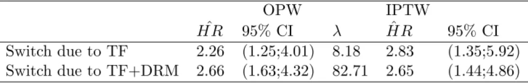
We set ξ equal to the value corresponding to the 20% increase in precision with respect to the standard error obtained by using IPW. We used a marginal structural Cox models weighted by IPW and OPW, to estimate the hazard ratio of treatment switch on time to second-line treatment failure. Table 4.1 shows the results of our analysis. We used robust standard errors (Freedman, 2006).
Table 4.1: Estimated hazard ratio of treatment switch on time to second-line treatment failure by using OPW and IPW.
OPW IPTW
ˆ
HR 95% CI λ HRˆ 95% CI Switch due to TF 2.26 (1.25;4.01) 8.18 2.83 (1.35;5.92) Switch due to TF+DRM 2.66 (1.63;4.32) 82.71 2.65 (1.44;4.86)
Note:HRˆ is the estimated hazard ration, CI is the confidence interval,λis the Lagrange multiplier associated with constraint 4.9. TF means treatment failure and DRM means drug resistance mutation.
We conclude that the there is a statistically significant effect of treatment switch on time to second-line HIV treatment. OPW provided similar results as those obtained with IPW but with higher precision.
Chapter 5
Discussion
Methods based on probability weighting have been subject of intense research in the field of statistics in the past decades, with applications in epidemiology, economics, and medicine. However, as shown the previous sections, these methods have several limitations. In this Ph.D. thesis we developed, evaluated and applied novel methods based on mathemati-cal programming techniques which aimed at providing optimal probability weights. The optimal probability weights proposed can be used to control for extreme weights in cross-sectional studies (Paper I), and in longitudinal studies (Paper II). In addition, we provided a novel method that simultaneously balance time-dependent confounders and control for extreme weights in longitudinal studies (Paper III). The method introduced in Paper III, emerged by the cross-pollination between causal inference, machine learning, and mathe-matical programming. This Ph.D. thesis work provided methods that will likely help to (1) extend the use of probability weighting methods in medicine, epidemiology, economics and social sciences, (2) extend knowledge on how mathematical programming and machine learning could be used to conduct robust analyses for improved decision-making, and (3) provide powerful, strong, and robust results to clinicians and policy-makers.
Chapter 6
Future research
Designing and developing novel methods for estimating causal effects which connects machine learning, statistics, personalization, and medicine has recently been recognized as an important and emerging field, with research groups worldwide studying and extending past knowledge regarding these methods. The following are ideas for future work.
Robust estimation of dynamic treatment regimes. Dynamic treatment regimes (DTR)s generalize personalized treatments in settings where treatments are time-varying, tailoring decisions based on the time-varying state of individual patients. Future research may focus on the development of methods that robustly estimate optimal DTRs in presence of time-dependent confounding. For instance, the performance of the optimal probability weights proposed in this Ph.D. thesis could be evaluated with popular methods to compare and find optimal DTRs, such as marginal structural models, and with novel learning methods that build upon the literature of statistical learning, such as backward outcome weighted learning (Zhao et al., 2015). In addition, future research may focus on the possible extensions to the evaluation of quantile optimal DTRs. Finally, future work may investigate the challenges and potential solutions to the issue of conducting inference for optimal DTRs (Chakraborty and Murphy, 2014; Chakraborty et al., 2010).
Stable weights for longitudinal censored data. Several methods have been developed to alleviate the presence of extreme weights when considering one single time point (Santacatterina et al., 2017; Zubizarreta, 2015, among others). However, when
esti-mating the causal effect of a time-varying treatment with longitudinal observational data few alternatives are available. Additionally, in longitudinal observational data, the outcome of interest may happen to be unobserved, due for example to loss of follow up. When the reasons for these losses are related to the study, selection bias is introduced. This phenomenon is usually called informative censoring. Although already partially addressed in Paper III, future research may focus on providing optimal weights with longitudinal data affected by time-dependent confounding and informative censoring.
6. Future research 25 Optimally balanced quantile treatment effects. The literature of causal inference has been focusing mainly on the average treatment effects. However, there is a vast area of problems where the interest is in investigating quantiles. In particular, formulating novel methods for DTRs in terms of quantiles allows the analyst to give a more comprehensive picture of the treatment effect on the outcome. Future research may focus on the development of methods that provide optimal weights to estimate quantile treatment effects.
Optimal covariate balance for non-binary treatments. Medical therapies and interven-tions commonly involve multiple and continuous treatments. For instance, more than twenty-five antiretroviral drugs in six classes are available for the treatment of HIV infection. An example of continuous treatment is the evaluation of the effect of red and processed meat intake on the risk of cardiovascular disease or cancer (McAfee et al., 2010). Future research may focus on the development of optimal weights, such as those presented in Paper III, that account for non-binary and continous treatments. For instance, when interested in continuous treatments, a proposal is to use a weighted kernel density estimator (wKDE) (Silverman, 1986), in which, similarly to Paper III, the expected value of the wKDE could be decomposed and minimized leading to optimal weights that balance covariates with respect of a continuous treatment. Constrained optimization for robust causal inference. In the past few years, several
methods have been proposed to stabilize probability weights when the positivity assumption is practically violated, which are embedded within the framework of constrained optimization. Among others, Zubizarreta (2015) suggested minimizing the variance of the weights while balancing covariates. Athey et al. (2016) introduced a more general estimator in case of high dimensions. Kallus (2016) proposed to use a set of probability weights that optimizes covariate balance while regularizing the resulting weights. Future research may evaluate and compare these methods in a comprehensive simulation study, propose extensions and novel formulations of some of the aforementioned methods and provide practical guidelines on the choice of the most suitable method when estimating causal effects in case of violations of the positivity assumption.
Optimal covariate balancing for high-dimensional causal inference. Several methods have been developed to estimate causal effects from non-experimental data under the assumptions of unconfoundedness and covariate overlap, also known as positiv-ity assumption. Popular examples include regression, inverse probabilpositiv-ity weighting, matching, and covariate balancing. These methods aim at balancing the distributions of the observed features across treated and control groups. In practice, to make the causal assumption of unconfoundedness plausible, investigators include a substantial number of features. However, in these settings, the assumption of covariate overlap is more difficult to satisfy. As a consequence, recently, there has been considerable
inter-26 6. Future research
est in extending the earlier literature on causal inference from non-experimental data to high-dimensional settings. Future research may focus on developing novel methods that balance covariates when using machine learning to estimate high-dimensional nuisances parameters, which can compensate for the bias of regularized regression adjustments, be a more robust alternative to inverse probability weighting, and ex-tend the proposed method to longitudinal settings where the estimation of the causal effect of a time-varying treatment is of interest. Furthermore, future research may explore the implications of overlap in high-dimensional non-experimental studies and investigate potential extensions to high-dimensional censored data.
References
Athey, S., G. W. Imbens, and S. Wager. 2016. Approximate Residual Balancing: De-Biased Inference of Average Treatment Effects in High Dimensions. ArXiv e-prints .
Athey, S., G. W. Imbens, S. Wager, et al. 2016. Efficient inference of average treatment effects in high dimensions via approximate residual balancing. Technical report. Bang, H., and J. M. Robins. 2005. Doubly robust estimation in missing data and causal
inference models. Biometrics 61(4): 962–973.
Basu, D. 2011. An Essay on the Logical Foundations of Survey Sampling, Part One.
In Selected Works of Debabrata Basu, ed. A. DasGupta, 167–206. Selected Works in
Probability and Statistics, Springer New York.
Beaumont, J.-F. 2008. A new approach to weighting and inference in sample surveys.
Biometrika 95(3): 539–553. URL http://biomet.oxfordjournals.org/content/95/
3/539
Beaumont, J.-F., D. Haziza, and A. Ruiz-Gazen. 2013. A unified approach to robust estimation in finite population sampling. Biometrika 100(3): 555–569. URL http: //biomet.oxfordjournals.org/content/100/3/555
Blackwell, M. 2013. A framework for dynamic causal inference in political science.American Journal of Political Science 57(2): 504–520.
Bottai, M., and J. Zhang. 2010. Laplace regression with censored data.Biometrical Journal
52(4): 487–503.
Cassel, C. M., C. E. S¨arndal, and J. H. Wretman. 1976. Some results on generalized differ-ence estimation and generalized regression estimation for finite populations. Biometrika
63(3): 615–620.
Chakraborty, B., S. Murphy, and V. Strecher. 2010. Inference for non-regular parameters in optimal dynamic treatment regimes. Statistical methods in medical research 19(3): 317–343.
Chakraborty, B., and S. A. Murphy. 2014. Dynamic treatment regimes. Annual review of statistics and its application 1: 447–464.
28 References
Chan, K. C. G., S. C. P. Yam, and Z. Zhang. 2016. Globally efficient non-parametric infer-ence of average treatment effects by empirical balancing calibration weighting. Journal of the Royal Statistical Society: Series B (Statistical Methodology) 78(3): 673–700. Cole, S. R., and M. A. Hern´an. 2008. Constructing inverse probability weights for marginal
structural models. American journal of epidemiology 168(6): 656–664.
Cox, B., and D. McGrath. 1981. An Examination of the Effect of Sample Weight Truncation on the Mean Square Error of Survey Estimates. Paper Presented at the 1981 Biometric
Society ENAR Meeting Richmond, VA, U.S.A.
Daniel, R., S. Cousens, B. De Stavola, M. Kenward, and J. Sterne. 2013. Methods for dealing with time-dependent confounding. Statistics in medicine 32(9): 1584–1618. Deville, J.-C., and C.-E. S¨arndal. 1992. Calibration estimators in survey sampling. Journal
of the American statistical Association 87(418): 376–382.
Elliot, M., and R. Little. 2000. Model-based alternatives to trimming survey weights.
Journal of Official Statistics 16(3): 191.
Elliott, M. R. 2009. Model Averaging Methods for Weight Trimming in Generalized Linear Regression Models. Journal of official statistics 25(1): 1–20. URL http://www.ncbi. nlm.nih.gov/pmc/articles/PMC3530169/
Foreman, E., and K. R. Brewer. 1971. The efficient use of supplementary information in standard sampling procedures. Journal of the Royal Statistical Society. Series B (Methodological) 391–400.
Freedman, D. A. 2006. On the so-called “Huber sandwich estimator” and “robust standard errors”. The American Statistician 60(4): 299–302.
Friedman, J., T. Hastie, and R. Tibshirani. 2001.The elements of statistical learning, vol. 1. Springer series in statistics New York.
Griva, I., S. G. Nash, and A. Sofer. 2009. Linear and nonlinear optimization, vol. 108. Siam.
Gruber, S., R. W. Logan, I. Jarr´ın, S. Monge, and M. A. Hern´an. 2015. Ensemble learning of inverse probability weights for marginal structural modeling in large observational datasets. Statistics in medicine 34(1): 106–117.
Hainmueller, J. 2012. Entropy balancing for causal effects: A multivariate reweighting method to produce balanced samples in observational studies. Political Analysis 20(1): 25–46.
Hern´an, M. ´A., B. Brumback, and J. M. Robins. 2000. Marginal structural models to estimate the causal effect of zidovudine on the survival of HIV-positive men.
References 29
Hern´an, M. A., B. Brumback, and J. M. Robins. 2001. Marginal structural models to estimate the joint causal effect of nonrandomized treatments. Journal of the American Statistical Association 96(454): 440–448.
Hernan, M. A., and J. M. Robins. 2010. Causal inference. CRC Boca Raton, FL:. Hirshberg, D. A., and S. Wager. 2017. Balancing Out Regression Error: Efficient Treatment
Effect Estimation without Smooth Propensities. ArXiv e-prints .
HIV-Causal Collaboration, et al. 2010. The effect of combined antiretroviral therapy on the overall mortality of HIV-infected individuals. AIDS (London, England) 24(1): 123. . 2011. When to initiate combined antiretroviral therapy to reduce mortality and AIDS-defining illness in HIV-infected persons in developed countries: an observational study. Annals of Internal Medicine 154(8): 509.
Hofmann, T., B. Sch¨olkopf, and A. J. Smola. 2008. Kernel methods in machine learning.
The annals of statistics 1171–1220.
Horvitz, D. G., and D. J. Thompson. 1952. A generalization of sampling without replace-ment from a finite universe. Journal of the American statistical Association 47(260): 663–685.
Hulliger, B. 1995. Outlier Robust Horvitz-Thompson Estimators 21(1): 79–87.
Imai, K., and M. Ratkovic. 2014. Covariate balancing propensity score. Journal of the Royal Statistical Society: Series B (Statistical Methodology) 76(1): 243–263.
. 2015. Robust estimation of inverse probability weights for marginal structural models. Journal of the American Statistical Association 110(511): 1013–1023.
Imbens, G. W., and D. B. Rubin. 2015.Causal inference in statistics, social, and biomedical sciences. Cambridge University Press.
Kallus, N. 2016. Generalized Optimal Matching Methods for Causal Inference. ArXiv e-prints .
Kang, J. D., and J. L. Schafer. 2007a. Demystifying double robustness: A comparison of alternative strategies for estimating a population mean from incomplete data. Statistical science 523–539.
Kang, J. D. Y., and J. L. Schafer. 2007b. Demystifying Double Robustness: A Comparison of Alternative Strategies for Estimating a Population Mean from Incomplete Data.
Statist. Sci. 22(4): 523–539. URLhttp://dx.doi.org/10.1214/07-STS227
Karim, M. E., J. Petkau, P. Gustafson, H. Tremlett, and T. B. S. Group. 2017. On the application of statistical learning approaches to construct inverse probability weights in
30 References
marginal structural cox models: Hedging against weight-model misspecification. Com-munications in Statistics-Simulation and Computation 1–30.
Karim, M. E., and R. W. Platt. 2017. Estimating inverse probability weights using super learner when weight-model specification is unknown in a marginal structural Cox model context. Statistics in Medicine 36(13): 2032–2047.
Koenker, R. 2011. A note on Laplace regression with censored data. Biometric Journal
53(5): 855–860.
Kokic, P., and P. Bell. 1994. Optimal winsorizing cutoffs for a stratified finite population estimator. Journal of Official Statistics 10(4): 419.
Kuhn, H. W. 1955. The Hungarian method for the assignment problem. Naval Research Logistics (NRL) 2(1-2): 83–97.
Lee, B. K., J. Lessler, and E. A. Stuart. 2010. Improving propensity score weighting using machine learning. Statistics in medicine 29(3): 337–346.
Lefebvre, G., J. A. Delaney, and R. W. Platt. 2008. Impact of mis-specification of the treatment model on estimates from a marginal structural model. Statistics in medicine
27(18): 3629–3642.
Li, F., K. L. Morgan, and A. M. Zaslavsky. 2017. Balancing covariates via propensity score weighting. Journal of the American Statistical Association 1–11.
Li, Y. P., K. J. Propert, and P. R. Rosenbaum. 2001. Balanced risk set matching. Journal of the American Statistical Association 96(455): 870–882.
Little, R. J., and D. B. Rubin. 2014. Statistical analysis with missing data, vol. 333. John Wiley & Sons.
Lodi, S., D. Costagliola, C. Sabin, J. del Amo, R. Logan, S. Abgrall, P. Reiss, A. van Sighem, S. Jose, J.-r. Blanco, et al. 2017. Effect of immediate initiation of antiretroviral treatment in HIV-positive individuals aged 50 years or older. Jaids Journal of Acquired
Immune Deficiency Syndromes .
Lu, B. 2005. Propensity score matching with time-dependent covariates. Biometrics61(3): 721–728.
Luenberger, D. G., and Y. Ye. 2015. Linear and Nonlinear Programming .
Lumley, T., P. A. Shaw, and J. Y. Dai. 2011. Connections between survey calibration estimators and semiparametric models for incomplete data. International Statistical
References 31
McAfee, A. J., E. M. McSorley, G. J. Cuskelly, B. W. Moss, J. M. Wallace, M. P. Bonham, and A. M. Fearon. 2010. Red meat consumption: An overview of the risks and benefits.
Meat science 84(1): 1–13.
Pfeffermann, D. 1993. The role of sampling weights when modeling survey data. Interna-tional Statistical Review/Revue InternaInterna-tionale de Statistique 317–337.
Pfeffermann, D., and M. Sverchkov. 1999. Parametric and Semi-Parametric Estimation of Regression Models Fitted to Survey Data. Sankhya: The Indian Journal of Statistics,
Series B (1960-2002) 61(1): 166–186. URL http://www.jstor.org/stable/25053074
Potter, F. 1990. A study of procedures to identify and trim extreme sampling weights. In
Proceedings of the American Statistical Association, Section on Survey Research Methods, vol. 225230.
Rao, J. N. K. 1966. Alternative Estimators in PPS Sampling for Multiple Characteristics.
Sankhya: The Indian Journal of Statistics, Series A (1961-2002) 28(1): 47–60. URL
http://www.jstor.org/stable/25049398
Rasmussen, C. E. 2004. Gaussian processes in machine learning. InAdvanced lectures on machine learning, 63–71. Springer.
Rivest, L.-P., D. Hurtubise, and Statistics Canada. 1995. On Searls’ winsorized mean for skewed populations. In Survey methodology, 107–116.
Robins, J. 1986. A new approach to causal inference in mortality studies with a sus-tained exposure period—application to control of the healthy worker survivor effect.
Mathematical modelling 7(9-12): 1393–1512.
Robins, J., M. Sued, Q. Lei-Gomez, and A. Rotnitzky. 2007. Comment: Performance of Double-Robust Estimators When “Inverse Probability” Weights Are Highly Variable.
Statist. Sci. 22(4): 544–559. URLhttp://dx.doi.org/10.1214/07-STS227D
Robins, J. M. 2000. Marginal structural models versus structural nested models as tools for causal inference. InStatistical models in epidemiology, the environment, and clinical trials, 95–133. Springer.
Robins, J. M., S. Greenland, and F.-C. Hu. 1999. Estimation of the causal effect of a time-varying exposure on the marginal mean of a repeated binary outcome. Journal of the American Statistical Association 94(447): 687–700.
Robins, J. M., A. Rotnitzky, and L. P. Zhao. 1994. Estimation of regression coefficients when some regressors are not always observed. Journal of the American statistical Association 89(427): 846–866.
32 References
. 1995. Analysis of semiparametric regression models for repeated outcomes in the presence of missing data. Journal of the american statistical association 90(429): 106–121.
Rosenbaum, P. R. 1989. Optimal matching for observational studies. Journal of the American Statistical Association 84(408): 1024–1032.
. 2002. Observational studies. InObservational studies, 1–17. Springer.
Rosenbaum, P. R., and D. B. Rubin. 1983. The central role of the propensity score in observational studies for causal effects. Biometrika 70(1): 41–55.
Santacatterina, M., R. Bellocco, A. S¨onneborg, A. Ekstr¨om, and M. Bottai. 2017. Optimal probability weights for estimating causal effects of time-varying treatment with marginal structural Cox models.
S¨arndal, C. E. 1980. On π-inverse weighting versus best linear unbiased weighting in probability sampling. Biometrika 67(3): 639–650.
Scharfstein, D. O., A. Rotnitzky, and J. M. Robins. 1999. Adjusting for nonignorable drop-out using semiparametric nonresponse models. Journal of the American Statistical Association 94(448): 1096–1120.
Sch¨olkopf, B., and A. J. Smola. 2002. Learning with kernels: support vector machines, regularization, optimization, and beyond. MIT press.
Seaman, S. R., and I. R. White. 2013. Review of inverse probability weighting for dealing with missing data. Statistical methods in medical research 22(3): 278–295.
Silverman, B. W. 1986. Density estimation for statistics and data analysis, vol. 26. CRC press.
Stuart, E. A., S. R. Cole, C. P. Bradshaw, and P. J. Leaf. 2011a. The use of propensity scores to assess the generalizability of results from randomized trials. Journal of the Royal Statistical Society: Series A (Statistics in Society) 174(2): 369–386.
. 2011b. The use of propensity scores to assess the generalizability of results from randomized trials. Journal of the Royal Statistical Society Series A 174(2): 369–386. URLhttp://onlinelibrary.wiley.com/doi/10.1111/j.1467-985X.2010.00673.x/ abstract
Tsiatis, A. 2007. Semiparametric theory and missing data. Springer Science & Business Media.
Valliant, R., J. A. Dever, and F. Kreuter. 2013. Practical tools for designing and weighting survey samples. Springer.