BDDs in a Branch & Cut Framework
?Bernd Becker1, Markus Behle2, Friedrich Eisenbrand2, and Ralf Wimmer1 1 Albert-Ludwigs-Universität, Georges-Köhler-Allee 51, 79110 Freiburg im Breisgau,
Germany,{becker,wimmer}@informatik.uni-freiburg.de
2 Max-Planck-Institut für Informatik, Stuhlsatzenhausweg 85, 66123 Saarbrücken, Germany, {behle,eisen}@mpi-sb.mpg.de
Abstract. Branch & Cut is today’s state-of-the-art method to solve0/1-integer linear programs. Important for the success of this method is the generation of strong valid inequalities, which tighten the linear programming relaxation of0/ 1-IPs and thus allow for early pruning of parts of the search tree.
In this paper we present a novel approach to generate valid inequalities for0/ 1-IPs which is based on Binary Decision Diagrams (BDDs). BDDs are a data-structure which represents0/1-vectors as paths of a certain acyclic graph. They have been successfully applied in computational logic, hardware verification and synthesis.
We implemented our BDD cutting plane generator in a branch-and-cut frame-work and tested it on several instances of the MAX-ONES problem and randomly generated0/1-IPs. Our computational results show that we have developed com-petitive code for these problems, on which state-of-the-art MIP-solvers fall short.
1
Introduction
Many industrial optimization problems can be formulated as an integer program. For-mally, an integer program deals with the maximization of a linear objective function c(1)x(1) +· · ·+c(n)x(n), where the variablesx(1), . . . , x(n)have to be integers and have to satisfymgiven linear inequalitiesai1x(1) +· · ·ainx(n)≤bifor1≤i≤m. A
special case of integer programming is 0/1 integer programming (0/1-IP), which arises if the variables are additionally restricted to attain values in{0,1}. It is a particularly important special case, since most combinatorial optimization problems are modeled with decision variables and thus are0/1-IPs.
The most successful method for0/1-IP, which is applied by all competitive com-mercial codes is branch-and-cut. This variant of branch-and-bound relies on the fact that the linear relaxation of a given0/1-IP can be efficiently solved. The linear relax-ation is the linear program which is obtained from the0/1-IP by relaxing the condition x(i) ∈ {0,1} to the condition0 ≤ x(i) ≤ 1for eachi ∈ {1, . . . , n}. The value of the linear programming relaxation can then be used as an upper bound in a branch-and-bound approach to solve the0/1-IP. In branch-and-cut, one additionally applies
cut-ting planes [8, 26] to improve the quality of the linear programming relaxation. Cutcut-ting
?This work was partly supported by the German Research Council (DFG) as part of the
Tran-sregional Collaborative Research Center “Automatic Verification and Analysis of Complex Systems” (SFB/TR 14 AVACS). Seewww.avacs.orgfor more information.
planes are inequalities which are valid for all feasible integer points, but not necessarily valid for the rational points which are feasible for the linear programming relaxation. Thus the incorporation of cutting planes improves the tightness of the linear relaxation and helps to prune parts of the branch-and-bound tree.
In theory a cutting plane can be easily infered from a fractional optimal solution to the linear programming relaxation. The strength of the cutting plane is however crucial for the performance of the branch-and-cut process. Classes of strong valid inequali-ties are for example knapsack-cover inequaliinequali-ties [2, 6, 11, 29], clique inequaliinequali-ties [21] the flow-cover inequalities [23, 24] or the mixed integer rounding cuts [21]. Knapsack-cover and flow-Knapsack-cover inequalities in particular are inequalities which are valid for the 0/1-points which satisfy one single constraint of the 0/1-IP. Up to now there is no satisfactory method available which generates valid inequalities for the0/1-solutions of two or more inequalities. This paper aims at a method for this algorithmic problem which is based on Binary Decision Diagrams, a datastructure which is widely used in computational logic, hardware verification and logic synthesis.
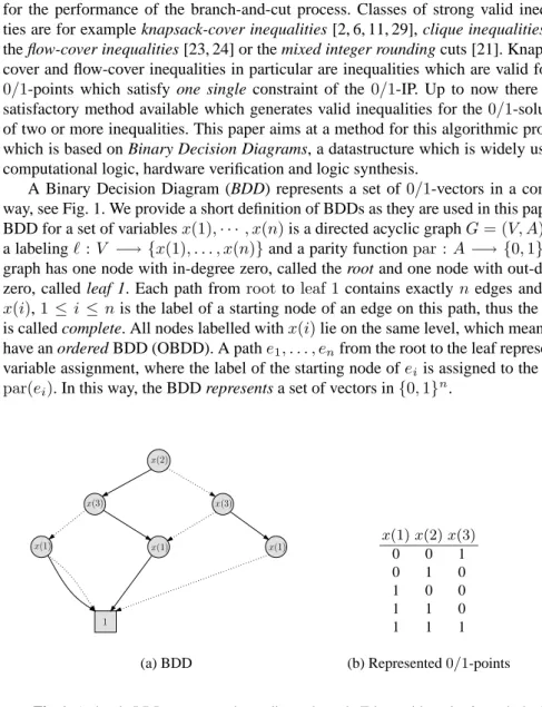
A Binary Decision Diagram (BDD) represents a set of0/1-vectors in a compact way, see Fig. 1. We provide a short definition of BDDs as they are used in this paper. A BDD for a set of variablesx(1),· · · , x(n)is a directed acyclic graphG= (V, A)with a labeling` :V −→ {x(1), . . . , x(n)}and a parity functionpar :A −→ {0,1}. The graph has one node with in-degree zero, called the root and one node with out-degree zero, called leaf 1. Each path fromroottoleaf 1contains exactlynedges and each x(i),1 ≤i ≤nis the label of a starting node of an edge on this path, thus the BDD is called complete. All nodes labelled withx(i)lie on the same level, which means, we have an ordered BDD (OBDD). A pathe1, . . . , enfrom the root to the leaf represents a
variable assignment, where the label of the starting node ofei is assigned to the value
par(ei). In this way, the BDD represents a set of vectors in{0,1}n.
1 x(2) x(3) x(3) x(1) x(1) x(1) (a) BDD x(1)x(2)x(3) 0 0 1 0 1 0 1 0 0 1 1 0 1 1 1 (b) Represented0/1-points
Fig. 1. A simple BDD represented as a directed graph. Edges with parity 0 are dashed.
BDDs were first proposed by Lee in 1959 [20]. Bryant [3] presented efficient algo-rithms for the synthesis of BDDs. After that, BDDs became very popular in the area of
hardware verification, and computational logics, see e.g. [28]. Lai et. al. [19, 18] have developed a branch-and-bound algorithm for0/1-IP that uses an extension of BDDs called EVBDDs. EVBDDs represent functionsf : {0,1}n −→ ZZ. So the EVBDDs
are used not only to represent the characteristic functions of the constraints but also for the constraints themselves. In this approach however, one has to build an EVBDD for the conjunction of all the constraints of the0/1-IP. In many cases this leads to an explosion in memory requirement.
We incorporate BDDs into a cutting plane engine and apply it in an integer pro-gramming solver. We use BDDs to represent the feasible solutions of a small subset of the given constraints and derive valid inequalities for the polytope which is described by these solutions. Thereby we avoid the explosion of the size of the BDD which hap-pens if the BDD represents all the constraints. The separation problem is solved with a sequence of shortest path problems with Lagrangean relaxation techniques. For this we use a standard BDD-package and apply our own efficient implementation of an acyclic shortest path algorithm on the BDD-datastructure. We apply our cutting plane framework to the MAX-ONES problem and to randomly generated0/1-IPs. Our compu-tational results show that we could develop competitive code to solve hard0/1-integer programming problems, on which state-of-the-art commercial branch-and-cut codes fall short.
Currently there is active and promising research in the field of combining techniques from computational logic and constraint programming with integer programming, see e.g. [5, 13]. We contribute further to this development by using BDDs sucessfully and for the first time in a cutting plane engine.
1.1 Preliminaries from Polyhedral Theory
Before we proceed we review some terminology from polyhedral theory, see e.g. [21, 26]. A polyhedronPis a set of vectors of the formP ={x∈IRn|Ax≤b}, for some matrixA∈IRm×n
and some vectorb∈IRm. The polyhedron is rational if bothAand bcan be chosen to be rational. IfP is bounded, thenPis called a polytope. An integral 0/1-polytope is a polytope that is the convex hull of a set of0/1-vectorsS ⊆ {0,1}n.
The integer hull PI of a polytope P is the convex hull of the integral vectors inP. The dimension dim(P)ofP is the dimension of its affine hull andP ⊆ IRn is
full-dimensional ifdim(P) =n.
An inequalitycTx≤δis valid forP if it is satisfied by all points inP. IfcTx≤δ
is valid andδ= max{cTx|x∈P}, it defines a faceF ={x∈P |cTx=δ}ofP.
The faceFis a facet ofP, ifdim(F) = dim(P)−1.
2
Using BDDs to Generate Cutting Planes
Suppose we have to solve a0/1-integer programming problem,
max{cTx:Ax≤b, x∈ {0,1}n} (1)
whereA∈ZZm×n,b∈ZZmandc∈ZZn. Our idea is now to choose a subsetA0
x≤b0
which satisfyA0
x≤b0
. We next distinguish between two0/1-polytopesPIandPBDD. The polytope PI = conv{x ∈ {0,1}n | Ax ≤ b}is the convex hull of the feasible 0/1-points of the0/1-IP. The polytopePBDD = conv{x∈ {0,1}n |A0x≤b0}is the convex hull of the0/1-points which are feasible forA0
x ≤ b0
. ClearlyPBDD ⊇PI. We are now interested in an efficient handling of the constraints which definePBDD. In a branch-and-cut framework, we want to decide whether our current optimal solution x∗
to the linear programming relaxation lies inPBDD. If not, we want to compute an inequality which is valid forPBDDbut not valid forx∗. This is the so-called separation
problem forPBDD.
BDD-SEP Givenx∗
∈Qnand a BDD(G, `,par), decide, whetherx∗
∈PBDDand if not, compute a valid inequality forPBDDwhich is not valid forx∗.
2.1 Polynomial Time Solvability of BDD-SEP
In the 1980’s, several authors[9, 17, 22] showed that the linear optimization problem over polyhedra and the separation problem over polyhedra are polynomial time equiva-lent. This equivalence of separation and optimization is a central result in combinatorial optimization. It implies that one can solve the separation problem forPBDDin polyno-mial time, if one can solve the optimization problem forPBDDin polynomial time.
BDD-OPT
Givenc∈Qnand a BDD(G, `,par), compute a0/1-point which is rep-resented by(G, `,par)and is maximal w.r.t. the linear objective function cTx.
BDD-OPT is easily shown to be the following longest path problem onGwith edge weightsw:E→IR, where
w(e) =
(
c(i) if par(e) = 1and`(head(e)) =x(i),
0 otherwise. (2)
It is very easy to see that the optimal solutions to BDD-OPT are exactly the 0/1-points which are represented by a longest path fromroottoleaf 1. SinceGis acyclic, the longest path problem can be solved in linear time. Using the equivalence of sepa-ration and optimization, we can thus conclude that BDD-SEP can, in theory, also be efficiently solved.
Theorem 1. The problems BDD-SEP and BDD-OPT can be solved in polynomial time.
2.2 Separation with the Subgradient Method
The pointx∗
/
∈PBDDif and only if there exists aλ∈IRnsuch that λTx∗
The valueδλis the length of the longest path fromroottoleaf 1w.r.t. the edge weights
wλ(e) =
(
λ(i) if par(e) = 1and`(head(e)) =x(i),
0 otherwise. (4)
SinceGis acyclic,δλcan be computed in linear time. If (3) does not hold, we updateλ
as in the subgradient method to solve the Lagrangean relaxation, see e.g. [26, p. 367ff.]. In words, Alg. 1 does the following. The first guess for a normalvector of a separating
Algorithm 1 Subgradient separation routine
(1) k:= 1 (2) λ(k):=c
(3) Compute a longest pathp(k)fromroottoleaf 1w.r.t. the edge lengthsw
λ(k).
(4) IfλTx∗> δ
λthen return the separating hyperplaneλTx≤δλ
(5) t(k):= 1 k (6) λ(k+1):=λ(k)+t(k)(x∗−x p(k)) (7) k := k + 1; (8) GOTO (3)
hyperplane is the objective function vectorc, which is whyλis initialized with this vector. Letλ(k)be the normalvector in thek-th iteration such thatλ(k)Tx∗
≤δλ(k) =
λ(k)Tx
p(k). After the update one has λ(k+1)
T (x∗ −xp(k)) = λ(k) T (x∗ −xp(k)) + t(k)kx∗
−xp(k)k2. Ift(k)>0is small enough then there exists a longest path w.r.t.wλ(k),
which is also a longest path w.r.t.wλ(k+1). Thenλ(k+1)
T x∗ −δλ(k+1)> λ(k) T x∗ −δλ(k).
It is known, see [26], that for anyt(k)withlim
k→∞t(k) = 0and P∞
k=1t(
k)=∞the subgradient method terminates. This is the case fort(k)= 1/k.
Geometrically, step 6 can be interpreted as a rotation of the hyperplaneλ(k)Tx≤δ
λ
in the direction of the vectorx∗
−xp(k). Although Alg. 1 cannot be guaranteed to run
in polynomial time, we observed that it outperforms linear programming methods for BDD-SEP by far. This is why we implemented this method in our BDD cut-separator.
3
Heuristics for Strengthening Inequalities with BDDs
The inequalities generated with the subgradient method naturally define faces ofPBDD with a low dimension. We want to increase their dimension in order to increase the “quality” of the hyperplanes, i.e., we are interested in facets ofPBDD. Using facet-defining inequalities in branch-and-cut has led to an enourmous progress in solving large-scale optimization problems, see e.g. [16]. The standard way to turn a separating hyperplane into a facet-defining inequality, see e.g. [10], turned out to be too expen-sive. Therefore, we developed some heuristics to strengthen inequalities which do not guarantee to produce facets, but can be efficiently implemented.
In the following letcTx≤δbe a valid inequality forP
BDD. The right hand side can be set toδ= max{cTx|x∈P
BDD}. We compute the maximum in linear time via optimizing overPBDDwith edge weights set towcas in (2). Note that with this method
every inequality can be made tight at at least one vertex of the BDD-polytope.
3.1 Increasing the Number of Tight Vertices
By increasing the number of vertices ofPBDD that are tight atcTx ≤δ, chances are high to also increase the dimension of the induced face. In the following we try to strengthen an inequality along the unit vectors. Remember that every path in the BDD-graph from theroottoleaf 1corresponds to a vertex ofPBDD. W.l.o.g. assume that for alli∈ {1, . . . , n}the variablex(i)lies in leveli.
Giveni∈ {1, . . . , n}we want to find a newc(i)so that the number of longest paths w.r.t. the edge weightswcincreases. For that we compute the sets of all longest paths,
that use a 0-edge resp. 1-edge in leveli. Beα0resp.α1their costs. Ifα06=α1setting c(i) :=c(i) +α0−α1andδ:=α0increases the number of shortest paths.
The strengthenedcdepends on the order of the indices which we took to strengthen it. Different permutations of{1, . . . , n}can lead to different strengthened hyperplanes. For the computation ofc(i)we look at each edge ofGonce. As we strengthen every coefficient ofcthe total running time isO(n|A|). If we do not consider permutations of the indices but take the canonical order{1, . . . , n}we only have to use each edge three times, so the running time can be reduced toO(|A|).
In a branch-and-cut framework it may occur that a hyperplane separating a givenx∗
does not separatex∗
after strengthening for an indexi. In this case we do not change c(i).
3.2 Improving Coefficients
In the following we adapted a strategy known for lifting cover inequalities for the knapsack problem, see e.g. [21]. W.l.o.g. assume that c ≥ 0holds. If there exists a c(i) < 0 replace δ := δ−c(i)andc(i) := −c(i). For simplicity reasons assume we want to strengthen c(1) which means, as we havex ≥ 0, increasing its value. Rewriting the inequality to c(1)x(1) ≤ δ−Pn
i=2c(i)x(i) shows that we can set c(1) := δ−max{Pn
i=2c(i)x(i) | x ∈ PBDD, x(1) = 1}. Again we use the fact that we can optimize overPBDDin linear time. Different permutations of indices again lead to different strengthened inequalities.
4
Computational Results
The cuts that we developed in this paper can be used for any0/1-integer program, even for those, where nothing is known about their structure. We investigated the practical strength of our theory by doing computational experiments. Our results with MAX-ONES problems and randomly generated IPs show, that one can achieve a considerable speedup on hard and small0/1-IPs. We report on some techniques that we developed to build BDDs fast and to keep their sizes small.
4.1 Heuristics for the Variable Order of the BDD
It is well-known that the variable order used in a BDD has a great influence on its size [28]. Before we start to build BDDs for any subsetA0
x≤b0
, we choose an appro-priate variable order, which considers all constraintsA x≤b.
Experiments have shown that heuristics that do not take the structure of the problem into account will produce bad variable orders. We adapted an algorithm for partition-ing the outputs of circuits that was presented in [12]. It proceeds as follows: First the constraint setA x≤bis partitioned into subsets with a similar support. Then, for every subset a partial variable order is computed. These partial orders are merged into one total order using a technique called interleaving [7].
For the partitioning of the constraints generate a new initially empty block. Delete that constraint from the set of constraints that has the largest support and insert it into the new block. This constraint is called the leader of the block. Then all constraints satisfying a certain criterion are moved to the new block. We iterate until the set of constraints becomes empty.
The two citeria we used are:
1. Add a constraint if its support is a subset of the support of the leader (WOG). 2. Add a constraint if its support is a subset of the supports of all constraints already
contained in the block (BOG).
For the partial orders we used a simple heuristics. For every variablex(j)we com-putedhj =P
n
i=1|aij|and sorted the variables in every block according to decreasing
hjvalue. Before we apply the interleaving algorithm we sort the blocks increasingly by
the number of variables contained in them.
Besides this algorithm that computes an inital variable order, we use sifting [25] to improve the order dynamically while we build the BDDs.
4.2 Building a BDD for a Subset of Constraints
We mainly use the following two operations for BDDs: computing the BDD for the
characteristic function of a single constraint and the conjunction of two BDDs. Both
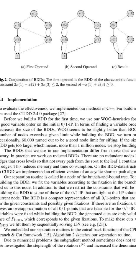
BDD algorithms work recursively. The top-most variable is set to 0 and 1 and the al-gorithm is called recursively on the two branches. Figure 2 shows an example of a conjunction of two BDDs.
4.3 Decreasing the Size of the BDD
LetaTx ≤ bbe a constraint of the0/1-IP, that has not been used to build the BDD.
We set the edge weights in the BDD-graph towaas in (2) and optimize over it. A point
xp∈PBDDsatifies the constraintaTx≤bif and only if the costs of its corresponding pathpare less or equalb. For a given node, consider the costs of all paths that cross it. If the minimum of these costs is greater thanb, we can delete that node together with its incident edges, since we are only interested in those points of the BDD-polytope, that satisfy the given constraint.
This algorithm runs in linear time in the number of nodes of the BDD and it can be applied while the BDD is built.
x(1) x(2) x(2) x(3) x(3) 1
(a) First Operand
x(1) x(2) x(2) x(3) x(3) 1 (b) Second Operand x(1) x(2) x(3) x(3) 1 (c) Result
Fig. 2. Conjunction of BDDs: The first operand is the BDD of the characteristic function of the constraint2x(1)−x(2) + 3x(3)≤2, the second of−x(1) +x(3)≥0.
4.4 Implementation
To evaluate the effectiveness, we implemented our methods in C++. For building BDDs we used the CUDD 2.4.0 package [27].
Before we build a BDD for the first time, we use our WOG-heuristics for finding a good variable order on the initial0/1-IP. In terms of finding a variable order which decreases the size of the BDDs, WOG seems to be slightly better than BOG. If the number of nodes exceeds a given limit while building the BDD, we turn on sifting occasionally. 60.000turned out to be a good node limit for sifting. If the size of the BDD gets too large, which means, more than 1 million nodes, we stop building it.
The BDDs that we use in our implementation differ from those that we use for theory. In practice we work on reduced BDDs. There are no redundant nodes but long edges that cross levels so that not every path from therootto theleaf 1contains exactly nedges. This reduces memory and time consumption. On the BDD-datastructure used in CUDD we implemented an efficient version of an acyclic shortest path algorithm.
Our separation routine is called in a node of the branch-and-bound tree. To simplify building the BDD, we fix the variables according to the fixation in the branching that led us to this node. In addition to that we restrict the constraints that will be used for building the BDD to some of those of the0/1-IP that are tight at the LP solution in the current node. The BDD is a compact representation of all0/1-points that are feasible for the given constraints and possibly given fixations. If there are no fixations, the BDD gives an overapproximation of all0/1-points that are feasible for the0/1-IP. If some variables were fixed while building the BDD, the generated cuts are only valid for that face ofPBDD, which corresponds to the given fixations. To make these cuts valid for PBDDwe lift them by sequentially solving LPs (see e.g. [21]).
We embedded our separation routines in the cutcallback function of the CPLEX 9.0 Branch & Cut framework [15]. Algorithm 2 sketches our separation routine.
Due to numerical problems the subgradient method sometimes does not terminate. We investigated the steplength of the rotationt(k)and increased the denominator by 1
Algorithm 2 Separation via BDDs as cutcallback function
(1) Restriction: Fix some variables according to the branching decisions.
(2) Build the BDD for some of the constraints that are tight at the LP solution.
(3) Solve the separation problem with the subgradient method.
(4) Strengthen the cuts.
(5) Lift the strengthened cuts into the original full space and return them.
not in every but in everys’th iteration wheres= 5showed to be a good value for most of the cases. If we cannot find a separating hyperplane after 2000 iterations we stop. To make the hyperplanes integer, we multiply them with an adequate integer value and round them. After that we compute a new right-hand-side via a shortest path computa-tion. In almost all of the cases the resulting integer hyperplanes are still separating the current LP solution from the0/1-IP.
4.5 Benchmarks
MAX-ONES Satisfiability problems notoriously produce hard to solve IPs [1].
There-fore we investigated SAT instances and converted them to MAX-ONES problems. A given SAT-instance overnboolean variables and a set of clausesC1, . . . , Ckcan easily
be transformed into a0/1-IP representing a MAX-ONES problem by converting each clause to a linear constraint of the formP
ix(i) +
P
j(1−x(j))≥1and adding the
objective functionmaxPn
i=1x(i). From a SAT competition held in 1992 [4], we took the hfo instances. The 5cnf instances are competition benchmarks of SAT-02 [14], and the remaining instances are competition benchmarks from SAT-03 [14].
Randomly Generated IPs Additionally we are interested in how our code performs
on problems with less or without any structure. We randomly generated0/1-IPs the following way: an entry in the matrixA, the right-hand-sideband the objective function c gets a nonzero value with probabilityp. This value is randomly chosen from the integers with absolute value less or equal cmax. The instances that we generated are available on request.
4.6 Results
Our experiments have been performed on a PC Intel Xeon CPU 3.06 GHz with 4 GByte RAM on GNU/Linux (kernel 2.6) operating system. Every investigated problem was solved to optimality or proved to be infeasible. On the one hand we run CPLEX 9.0 with the default values, i.e. it did presolving and used all types of built-in separation cuts. On the other hand we used the CPLEX Branch & Cut framework with our separa-tion routines (bcBDD), but switched off presolve and all built-in cuts. We switched off presolve since we sometimes encountered problems working on the presolved model. We also tried to switch off presolve for the benchmarks made with CPLEX standalone. It showed, that presolving the randomly generated IPs does not really influence the run-ning time but switching off presolve for the MAX-ONES instances increased CPLEX running times.
For the MAX-ONES instances we found out, that generating nearly all of our cuts in the root node is the most promising strategy. Using too few constraints to build the BDD resulted in weaker cutting planes. In practice it showed that 70% of the constraints, that are tight at the current LP solution, is a good threshold for generating cuts with an adequate quality while building the BDD does not consume too much time.
For randomly generated IPs building the BDDs is harder as the constraints have no structure. We generated our cuts deeper in the branch-and-bound tree and lifted them. Furthermore we only used 20% of the constraints, that belong to the basis of the LP solution in the current branch-and-bound node.
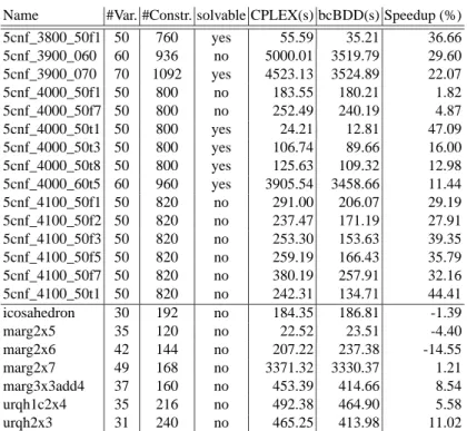
Table 1. Results for the SAT-02 / SAT-03 instances
Name #Var. #Constr. solvable CPLEX(s) bcBDD(s) Speedup (%) 5cnf_3800_50f1 50 760 yes 55.59 35.21 36.66 5cnf_3900_060 60 936 no 5000.01 3519.79 29.60 5cnf_3900_070 70 1092 yes 4523.13 3524.89 22.07 5cnf_4000_50f1 50 800 no 183.55 180.21 1.82 5cnf_4000_50f7 50 800 no 252.49 240.19 4.87 5cnf_4000_50t1 50 800 yes 24.21 12.81 47.09 5cnf_4000_50t3 50 800 yes 106.74 89.66 16.00 5cnf_4000_50t8 50 800 yes 125.63 109.32 12.98 5cnf_4000_60t5 60 960 yes 3905.54 3458.66 11.44 5cnf_4100_50f1 50 820 no 291.00 206.07 29.19 5cnf_4100_50f2 50 820 no 237.47 171.19 27.91 5cnf_4100_50f3 50 820 no 253.30 153.63 39.35 5cnf_4100_50f5 50 820 no 259.19 166.43 35.79 5cnf_4100_50f7 50 820 no 380.19 257.91 32.16 5cnf_4100_50t1 50 820 no 242.31 134.71 44.41 icosahedron 30 192 no 184.35 186.81 -1.39 marg2x5 35 120 no 22.52 23.51 -4.40 marg2x6 42 144 no 207.22 237.38 -14.55 marg2x7 49 168 no 3371.32 3330.37 1.21 marg3x3add4 37 160 no 453.39 414.66 8.54 urqh1c2x4 35 216 no 492.38 464.90 5.58 urqh2x3 31 240 no 465.25 413.98 11.02
In all tables the running times are the total user times given in seconds. We com-puted the speedup as 1 minus the ratio of our running time divided by the CPLEX running time. The values for the hfo instances are average values taken over 20 differ-ent instances of each type. The standard deviation is in brackets. For 109 of the 120 hfo-instances we obtain faster running times compared to CPLEX default MIP-solver. The average of the overall speedup for the hfo-instances is 18.31% with a standard de-viation of 14.44%. For the randomly generated IPs we achieved an average speedup of 34.23%.
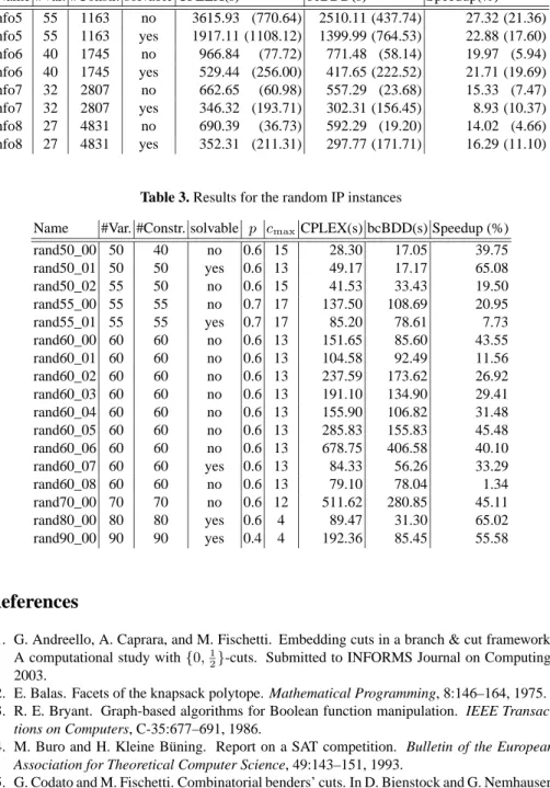
Table 2. Results for the hfo instances
Name #Var. #Constr. solvable CPLEX(s) bcBDD(s) Speedup(%) hfo5 55 1163 no 3615.93 (770.64) 2510.11 (437.74) 27.32 (21.36) hfo5 55 1163 yes 1917.11 (1108.12) 1399.99 (764.53) 22.88 (17.60) hfo6 40 1745 no 966.84 (77.72) 771.48 (58.14) 19.97 (5.94) hfo6 40 1745 yes 529.44 (256.00) 417.65 (222.52) 21.71 (19.69) hfo7 32 2807 no 662.65 (60.98) 557.29 (23.68) 15.33 (7.47) hfo7 32 2807 yes 346.32 (193.71) 302.31 (156.45) 8.93 (10.37) hfo8 27 4831 no 690.39 (36.73) 592.29 (19.20) 14.02 (4.66) hfo8 27 4831 yes 352.31 (211.31) 297.77 (171.71) 16.29 (11.10)
Table 3. Results for the random IP instances
Name #Var. #Constr. solvable p cmaxCPLEX(s) bcBDD(s) Speedup (%) rand50_00 50 40 no 0.6 15 28.30 17.05 39.75 rand50_01 50 50 yes 0.6 13 49.17 17.17 65.08 rand50_02 55 50 no 0.6 15 41.53 33.43 19.50 rand55_00 55 55 no 0.7 17 137.50 108.69 20.95 rand55_01 55 55 yes 0.7 17 85.20 78.61 7.73 rand60_00 60 60 no 0.6 13 151.65 85.60 43.55 rand60_01 60 60 no 0.6 13 104.58 92.49 11.56 rand60_02 60 60 no 0.6 13 237.59 173.62 26.92 rand60_03 60 60 no 0.6 13 191.10 134.90 29.41 rand60_04 60 60 no 0.6 13 155.90 106.82 31.48 rand60_05 60 60 no 0.6 13 285.83 155.83 45.48 rand60_06 60 60 no 0.6 13 678.75 406.58 40.10 rand60_07 60 60 yes 0.6 13 84.33 56.26 33.29 rand60_08 60 60 no 0.6 13 79.10 78.04 1.34 rand70_00 70 70 no 0.6 12 511.62 280.85 45.11 rand80_00 80 80 yes 0.6 4 89.47 31.30 65.02 rand90_00 90 90 yes 0.4 4 192.36 85.45 55.58
References
1. G. Andreello, A. Caprara, and M. Fischetti. Embedding cuts in a branch & cut framework: A computational study with{0,1
2}-cuts. Submitted to INFORMS Journal on Computing, 2003.
2. E. Balas. Facets of the knapsack polytope. Mathematical Programming, 8:146–164, 1975. 3. R. E. Bryant. Graph-based algorithms for Boolean function manipulation. IEEE
Transac-tions on Computers, C-35:677–691, 1986.
4. M. Buro and H. Kleine Büning. Report on a SAT competition. Bulletin of the European
Association for Theoretical Computer Science, 49:143–151, 1993.
5. G. Codato and M. Fischetti. Combinatorial benders’ cuts. In D. Bienstock and G. Nemhauser, editors, Integer Programming and Combinatorial Optimization, IPCO X Proceedings, Lec-ture Notes in Computer Science, pages 178–195. Springer, 2004.
6. H. Crowder, E. J. Johnson, and M. Padberg. Solving large-scale 0-1 linear programming problems. Operations Research, 31(5):803–834, 1983.
7. H. Fujii, G. Ootomo, and C. Hori. Interleaving based variable ordering methods for ordered binary decision diagrams. In Proceedings of the IEEE/ACM International Conference on
Computer-Aided Design, pages 38 – 41, 1993.
8. R. E. Gomory. Outline of an algorithm for integer solutions to linear programs. Bulletin of
the American Mathematical Society, 64:275–278, 1958.
9. M. Grötschel, L. Lovász, and A. Schrijver. The ellipsoid method and its consequences in combinatorial optimization. Combinatorica, 1(2):169–197, 1981.
10. M. Grötschel, L. Lovász, and A. Schrijver. Geometric Algorithms and Combinatorial
Opti-mization, volume 2 of Algorithms and Combinatorics. Springer, 1988.
11. P. L. Hammer, E. Johnson, and U. N. Peled. Facets of regular 0-1 polytopes. Mathematical
Programming, 8:179–206, 1975.
12. M. Herbstritt, T. Kmieciak, and B. Becker. On the impact of structural circuit partitioning on SAT-based combinational circuit verification. In Proceedings of 5th IEEE International
Workshop on Microprocessor Test and Verification, Austin, USA, 2004.
13. J. N. Hooker. Planning and scheduling by logic-based benders decomposition. Working paper, 2004.
14. H. H. Hoos and T. Stützle. SATLIB: An online resource for research on SAT. In I. P. Gent and T. Walsh, editors, Satisfiability in the year 2000, pages 283–292. IOS Press, 2000. 15. ILOG. CPLEX 9.0 User’s Manual and Reference Manual. S.A., 2003.
16. M. Jünger, G. Reinelt, and G. Rinaldi. The traveling salesman problem. In Handbook on
Operations Research and Management Science, volume 7, pages 225–330. Elsevier, 1995.
17. R. M. Karp and C. H. Papadimitriou. On linear characterizations of combinatorial optimiza-tion problems. In 21st Annual Symposium on Foundaoptimiza-tions of Computer Science, pages 1–9. IEEE, New York, 1980.
18. Y. T. Lai, M. Pedram, and S. B. K. Vrudhula. FGILP: an integer linear program solver based on function graphs. In Proceedings of the IEEE/ACM International Conference on
Computer-Aided Design, pages 685–689, 1993.
19. Y. T. Lai, M. Pedram, and S. B. K. Vrudhula. EVBDD-based algorithms for integer lin-ear programming, spectral transformation, and functional decomposition. IEEE Trans. on
Computer-Aided Design, 13(8):959–975, 1994.
20. C. Y. Lee. Representation of switching circuits by binary-decision programs. The Bell
Systems Technical Journal, 38:985 – 999, 1959.
21. G. L. Nemhauser and L. A. Wolsey. Integer and Combinatorial Optimization. John Wiley, 1988.
22. M. W. Padberg and M. R. Rao. The russian method for linear programming III: Bounded integer programming. Technical Report 81-39, New York University, Graduate School of Business and Administration, 1981.
23. M. W. Padberg, T. J. Van Roy, and L. A. Wolsey. Valid linear inequalities for fixed charge problems. Operations Research, 33(4):842–861, 1985.
24. M. W. Padberg and L. A. Wolsey. Fractional covers for forests and matchings. Mathematical
Programming, 29(1):1–14, 1984.
25. R. Rudell. Dynamic variable ordering for ordered binary decision diagrams. In Proceedings
of the IEEE/ACM International Conference on Computer-Aided Design, pages 42–47, 1993.
26. A. Schrijver. Theory of Linear and Integer Programming. John Wiley, 1986.
27. F. Somenzi. CU Decision Diagram Package Release 2.4.0. Department of Electrical and Computer Engineering, University of Colorado at Boulder, 2004.
28. I. Wegener. Branching programs and binary decision diagrams. SIAM Monographs on Discrete Mathematics and Applications. SIAM, Philadelphia, PA, 2000.
29. L. A. Wolsey. Faces for a linear inequality in 0-1 variables. Mathematical Programming, 8:165–178, 1975.