Simulation methods for system reliability using the survival signature.

(1)

Durham Research Online

Deposited in DRO:

14 June 2017

Version of attached le:

Accepted Version

Peer-review status of attached le:

Peer-reviewed

Citation for published item:

Patelli, E. and Feng, G. and Coolen, F.P.A. and Coolen-Maturi, T. (2017) 'Simulation methods for system reliability using the survival signature.', Reliability engineering system safety., 167 . pp. 327-337.

Further information on publisher's website:

https://doi.org/10.1016/j.ress.2017.06.018 Publisher's copyright statement:

c

2017. This manuscript version is made available under the CC-BY-NC-ND 4.0 license

http://creativecommons.org/licenses/by-nc-nd/4.0/

Additional information:

Use policy

The full-text may be used and/or reproduced, and given to third parties in any format or medium, without prior permission or charge, for personal research or study, educational, or not-for-prot purposes provided that:

• a full bibliographic reference is made to the original source

• alinkis made to the metadata record in DRO

• the full-text is not changed in any way

The full-text must not be sold in any format or medium without the formal permission of the copyright holders. Please consult thefull DRO policyfor further details.

(2)

Simulation Methods for System Reliability Using the

Survival Signature

Edoardo Patelli1,⇤_{, Geng Feng}1_{, Frank P.A. Coolen}2_{, Tahani Coolen-Maturi}3 1_{Institute for Risk and Uncertainty, University of Liverpool, Liverpool, United Kingdom}

2_{Department of Mathematical Sciences, Durham University, Durham, United Kingdom} 3_{Durham University Business School, Durham University, Durham, United Kingdom}

Abstract

Recently, the survival signature has been presented as a summary of the structure function which is sufficient for computation of common reliability metrics and has the crucial advantage that it can be applied to systems with components whose failure times are not exchangeable. The survival signature provides a huge reduc-tion in required informareduc-tion, e.g. for its storage, compared to the full structure function, its implementation to larger systems is still difficult in a purely analyt-ical manner and simulations may be required to derive the reliability metrics of interest. Hence, the main question addressed in this paper is whether or not the survival signature provides sufficient information for efficient simulation to derive the system’s failure time distribution. We answer this question in the affirmative by presenting two algorithms for survival signature-based simulation. In addition, we present a third simulation algorithm that can be used in case of repairable com-ponents. It turns out that these algorithms are very efficient, beyond the initial advantage of requiring only the survival signature to be available, instead of the full structure function.

Keywords: Reliability Analysis; Survival Signature; Monte Carlo Method;

Complex Systems; Multi state components.

1. Introduction

The study of the reliability of complex systems, particularly systems with a structure that cannot be sequentially reduced by considering alternative series and parallel subsystems, is a topic subject which has attracted much attention in

⇤_{Corresponding author}

(3)

the literature and which is of obvious importance in many application areas [1].

5

Traditionally, the reliability analysis of systems is performed adopting di↵erent well-known tools such as reliability block diagrams, fault tree and success tree methods, failure mode and e↵ect analysis, and master logic diagrams [2]. The main limitation of these traditional approaches for applicability to large complex systems is due to the complex and tedious calculations for finding minimal path sets and

10

cut sets. For instance, for a system with m components 2m _{combinations of} component states must be specified, which is impossible for most practical systems and networks. Instead, if the systems components can be divided into groups with exchangeable failure times, the survival signature is sufficient to derive the systems failure time distribution given the components failure time distributions.

15

In addition, when the information about the system is not perfect, for example leading to imprecise probabilities being required to quantify the uncertainties, it is even more difficult to apply those methods.

In recent years, the system signature has been recognized as a useful tool to quantify the reliability of systems consisting of independent and identically

dis-20

tributed (iid) or exchangeable components with respect to their random failure times [3, 4], we say that such systems only have ‘components of one type’. The system signature enables full separation of the system structure from the compo-nent probabilistic failure time distribution when deriving the system failure time distribution. However, attempting to generalize the system signature to systems

25

with more than one component type is not really possible as it requires the compu-tation of the probabilities of di↵erent orderings of order statistics of the di↵erent failure time distributions involved [5], which tends to be intractable.

In order to overcome the limitations of the system signature, Coolen and Coolen-Maturi [5, 6] presented the survival signature, which has the same merits

30

as the system signature for systems consisting of a single type of components, but it is also an e↵ective tool for analysing complex systems consisting of multiple component types. Therefore, the survival signature is a useful tool for reliability quantification for complex systems and networks because it only needs to be calcu-lated once providing a massive reduction of the computational cost required by the

35

analysis. Recently, Coolen et al. [7] presented non-parametric predictive inference for system reliability using the survival signature, and Aslett et al. [8] did similarly within the Bayesian framework of statistics. Feng et al. [9] developed an analytical method to calculate the survival function of systems with uncertainty about pa-rameters of assumed component failure time distributions. These methods are all

40

useful, but may become less practical for larger complex systems. System survival signature can also be derived from subsystems’ survival signatures, if these are in

(4)

series-parallel configurations [7]. Recently, Reed presented and efficient computa-tional approach for computing exact system and survival signatures of large and complex systems [10]. The survival signature together with the provided

simula-45

tion algorithms provides a generalized tool for realistic quantification of system reliability.

Parameter uncertainties and imprecisions are generally epistemic in nature due to the lack of knowledge or data, or the unknown relationship between components (e.g., poor understanding of accident initiating events or coupled physics

phenom-50

ena, lack of data to characterise experiment processes, random errors in measuring and analytic devices), all of them make it difficult to characterize probabilistically the failure time of components. Since the reliability and performance of systems are directly a↵ected by uncertainties and imprecisions, a quantitative assessment of uncertainty is widely recognized as an important task in practical engineering

55

[11, 12].

Simulation approaches are used to investigate large and complex systems and for obtaining numerical solutions where analytical solutions are not available. In particular, simulation methods allow to consider explicitly the e↵ect of uncertainty and imprecision on the system under investigation providing a powerful tool for

60

risk analysis which allows better decision making under uncertainty. Simulation method can be used to e.g. identify problems before implementation, evaluate ideas and identify inefficiencies, understand why observed events occur.

The use of simulation methods for system reliability has many attractive fea-tures. Generally, it can be used for the sensitivity analysis of multi-criteria decision

65

model [13], optimize models with rare events [14] and perform multi-attribute de-cision making [15]. Most of the current simulation methods are based on Monte Carlo simulation and structure function. By generating the state evolution of each component, the structure function is computed to determine the state of the sys-tem. The structure function is in a boolean format and can only be used to identify

70

a specific output of the system. More structure functions can be used to match all the possible status of the system at the cost of increasing the complexity of the analysis (see e.g. [16]). Several methods are available for the reliability analysis of complex system based on structural function (see e.g. [17, 4, 18]). However, we envisage a scenario, particularly for large systems, where the full system structure

75

information (or structure function, min paths sets etc.) is not available but only the survival signature that represents a summary of the structure function. In particular, for very large scale systems and networks, storing only the survival signature and not the entire structure function is clearly advantageous.

In this paper, we will show that the survival signature is sufficient for basic

(5)

reliability inferences (e.g. determining the system reliability function) which can be used for further inferences and decision support. Efficient simulation approaches are proposed to estimate the reliability of systems based on survival signature. The method is particularly useful when the probability term of the survival function (as shown later in the Eq. 2 representing the probability of the components working

85

at specific time), cannot easily be derived analytically but the failure times for the exchangeable components can nevertheless be sampled through simulation.

The proposed simulation approaches are generally applicable to any system configuration. In addition, it allows to consider di↵erent representation of the un-certainties including system multi-state components (i.e. repairable components).

90

The numerical implementation of the proposed approaches is based on two open source packages: the R package “ReliabilityTheory” [19, 20] adopted to calculate the survival signature and OpenCossan [21, 22] a Matlab toolbox for uncertainty quantification and reliability analysis used to simulate the system evolution. The applicability and efficiency of the proposed approaches are demonstrated by

solv-95

ing numerical examples.

This paper is organized as follows. Section 2 presents a brief overview of the survival signature and the related system survival function. Survival signature-based simulation methods for system reliability are presented in Section 3. In Section 4, the applicability and performance of the proposed approaches is shown

100

by analysing four numerical examples. Finally Section 5 closes the paper with conclusions.

2. Survival Signature

Suppose there is one system consisting ofmcomponents. Let the state vector of components bex= (x1, x2, ..., xm)2{0,1}mwith xi = 1 if theith component

105

is in working state and xi = 0 if not. = (x) : {0,1}m ! {0,1} defines the system structure function, i.e., the system status based on all possible x. is 1 if the system functions for state vectorxand 0 if not.

Now consider a system withK 2 types ofM components, withmkindicating the number of components of each type andPK_k₌₁mk =M. It is assumed that the

110

failure times of the components of the same type are independently and identically distributed (iid) or exchangeable. Note that this is usually understood as implying that the components are ‘exchangeable’, e.g. produced by the same manufacturer. However, the assumed exchangeability of their failure times also implies a similarity of the tasks the components of the same type perform in the system, e.g. if similar

115

components function at di↵erent stress levels their failure time distributions are likely not to be the same and hence for the reliability analysis using the survival signature such components would be considered to be of di↵erent types. The

(6)

components of the same type can be grouped together because of the random ordering of the components in the state vector, which leads to a state vector can be

120

written as x= (x1_{, x}2_{, ..., x}K_{), with}_xk _{= (}_xk

1, xk2, ..., xkmk) representing the states

of the components of typek. Coolen and Coolen-Mature [5] introduced the survival signature for such a system, denoted by (l1, l2, ..., lK), withlk = 0,1, ..., mk for k = 1,2, ..., K, which is defined to be the probability that the system functions given that lk of its mk components of type k work, for each k 2 {1,2, ..., K}.

125 There are mk lk state vectorsx k _{with precisely} _l k components xki equal to 1, so with Pmk

i=1xki = lk (k = 1,2, ..., K), and Sl1,l2,...,lK denote the set of all state

vectors for the whole system.

Assume that the random failure times of components of the di↵erent types are fully independent, and in addition the components are exchangeable within the

130

same component types, then the survival signature is equal to:

(l1, ..., lK) = "_K Y k=1 ✓ mk lk ◆ 1# ⇥ X x2Sl1,l_2,...,lK (x), (1)

whereCk(t)2{0,1, ..., mk}is the number ofkcomponents working at timet. The survival function of the system withK types of components can be expressed as [5]: P(TS> t) = m1 X l1=0 ... mK X lK=0 (l1, ..., lK)P( K \ k=1 {Ck(t) =lk}) (2) If one can assume that the components of the same type have a known CDF,Fk(t)

135

for typek, and that the failure times of di↵erent component types are independent, then these expressions are simplified using [5]:

P( K \ k=1 {Ck(t) =lk}) = K Y k=1 P(Ck(t) =lk) = K Y k=1 ✓_m k lk ◆ [Fk(t)]mk lk_[1 _F_k(_t_)]lk (3) Equation (2) separates the structure of the system from the failure time distri-bution of its components, which is the main advantage of the survival signature, which it shares with the system signature. The survival signature only needs to

140

be calculated once for any system, which is similar to the system signature for systems with only single type of components. The survival signature is closely related with system signature. For a special case of a system with only one type (K = 1) of components, the survival signature and the system signature [3] are directly linked to each other through a simple equation, however, the latter cannot

(7)

be easily generalized for systems with multiple types (K 2) of components [5]. This implies that all attractive properties of the system signature also hold for the method using the survival signature. The survival signature is easy to apply for systems with multiple types of components, and one could argue it is much easier to interpret than the system signature. In addition, the quite

150

simple survival signature (in particular for large systems with only relatively few di↵erent component types) and its monotonicity for coherent systems provide clear advantages to work towards approximations of the system reliability metrics. This does not limit the applicability of the survival signature to non-coherent systems (for example, electric distribution network or part of the electronic equipment

155

of safety features). In such cases, the analysis of system with imprecision in the component failure time requires a full “double loop” approach as detailed in Section 3.4.

3. Simulation Methods

Exact analytical solution can be obtained from Eq. 2 and Eq. 3. However,

160

analytical solutions are restricted to particular cases (e.g. system with component failure time following exponential distribution and not repairable components). Instead, simulation methods can be applied to study and analyse any systems without introducing simplifications or unjustified assumptions.

The survival signature presented in the previous section can be adopted in a

165

Monte Carlo based simulation method to estimate the system reliability in a simple and efficient way. A possible system evolution is simulated by generating random events (i.e. the random transition such as failure times of the system components) and then estimating the status of the system based on the survival signature (Equation 3). Then, counting the occurrence number of a specific condition (e.g.

170

counting how many times the system is in working status), it is possible to estimate the reliability of the system. In this section, three Monte Carlo simulation methods adopting the survival signature are presented. The Algorithms 1 and 2 are used to estimate the reliability of non-repairable systems while Algorithm 3 can be applied for repairable systems and multi-state components as well.

175

3.1. Algorithm 1

The first simulation method is based on the realizations of failure events of the system’s components. For each failure event the status of the system is generated based on the probability that the system is working knowing that a specific number of components are working. Such probability is given by the survival signature

180

as defined in Equation (1). The survival signature is computed only once before starting the Monte Carlo simulation for instance using the approach presented in [10]. Suppose there is a system with Ccomponents, K component types andmk

(8)

components of typek. Hence,C=PK_k₌₁mk. We assume that components of type k have the same failure time distribution and that there is no repair opportunity

185

for the components. The reliability of the system can be estimated adopting the following procedure:

Step 0. Initialise variables and counters (i.e. V r);

Step 1. Sample the failure times for each component, fi, for i= 1,2, . . . , C. The failure time of a component of type k is obtained by sampling from the

190

corresponding CDFFk;

Step 2. Order the sequence of failure timestiti+1fori= 1,2, . . . , M. Hence,t1

represents the first failure of a system component,t2represents the second

failure and so on;

Step 3. At each failure time, it is easy to calculate the number of components

195

working for each component type: Ck(ti);

Step 4. Evaluate the survival signature which applies immediately after the cor-responding failure indicated as ti ⌘ (C1(ti), C2(ti), . . . , CK(ti));

Step 5. Drawn from a Bernoulli distribution with probability 1 t1 the system

status X1 at timet1, ifX1= 1 the system fails; 200

Step 6. If the system does not fail at t1, then consider t2. The probability that

the system functions at timet2is t2/ t1 =q2, given that it has survived

at timet1. So the system failure at timet2,X2, is drawn from a Bernoulli

distribution with the probability 1 q2;

Step 7. Repeat Step 6 to process other failure times: Seti=i+ 1 .

205

Step 8. Store the status of the system over the time, as follows: V r(j) =V r(j) + 1 8j :j·dt < tf where tf is the system failure time anddt represents the discretisation time.

The above procedure is repeated for N samples and the estimate of the survival function is obtained by averaging the vector collecting the status of the system

210

over the number samples: P(Ts> t)⇡V r_N(t).

This method simulates one system failure time in each run (Steps 1-7). It should be noted that with the assumption that the system fails if no component functions, this implies that there is ani⇤_{, less than or equal to}_C_{, such that}_q

i⇤ = 0.

Hence the system fails certainly at thisti⇤ if it has not failed before. 215

A pseudo-algorithms of the simulation method is shown in Algorithm 1.

3.2. Algorithm 2

It is possible to estimate the system reliability without the necessity to sample the system status at each component failure time. The idea is to interpret the survival signature as a normalised “production capability” of the system defined

(9)

by the Equation (1). For instance, if all the components are working, the system output is 1. If all components are in failure status, the system output is 0. Hence, instead of sampling the system state at each failure time, the survival signature is evaluated to collect the “production level of the system”, i.e. the survival signature is evaluated immediately after each sampled component failure time and collected

225

in proper counters. This can be obtained adopting the Algorithm 2 derived from the approach proposed by one of the authors used to estimated the production availability of an o↵shore installation requiring the derivation of the complete status of the system (based on the structural function and cut-sets) [16]. Here, a novel algorithm is proposed to estimate the reliability adopting the survival

230

signature and hence avoiding the tedious calculation of all the system status. The reliability of the system can be estimated modifying the Steps 5-7 of the Algorithm 1 as follows:

Step 5’. Compute the production level of the system by evaluating the survival signature at each time of interest ti. The probability that the system 235

survives timet1 is t1;

Step 6’. Collect the value of the survival signature in the vector V rrepresenting the survival function as follows: V r(j) = V r(j) + ti 8j : j·dt < ti

wheredtrepresents the discretization time.

The above procedure is repeated forN samples and the reliability of the system is

240

computed by averaging the values of the survival signature: P(Ts> t)⇡ _N1V r(t). The uses of the survival signature makes this approach extremely efficient since it does not require to sample the system output at each component transition time (i.e. component failures). For each Monte Carlo simulation, this method generates a random grid of time points at which to evaluate the survival signature

245

representing the survival probability of the system at those times. Finally, the survival function is obtained by directly averaging the survival signature over the time.

A pseudo-algorithms of the simulation method for non-repairable components is shown in Algorithm 2 and the flow chart of the simulation methods proposed

250

for estimate the reliability of non-repairable systems is shown in Figure 1a. Algorithm 2 follows the productivity idea, which gives each run a possible survival function while Algorithm 1 gives a single system failure time in each run. Therefore, Algorithm 1 is useful for inference where one explicitly wants the simulated system failure times, whilst Algorithm 2 is efficient for inference on the

255

system survival function.

(10)

Compute Survival Signature Φ

Sample component failure times

Update component status Ck Start N Monte Carlo simulations

Process next time

i=i+1 System

working? Collect system status

(1s from 0 to ti)

Process failure time ti

Collect "production level"

Φ(C1,C2, ..., Ck) for ti-1 to ti Compute probability qi

Sample system status Bernoulli distribution Algorithm 1 Algorithm 2 Yes No Yes Process next sample Yes

Compute survival function

(a) Flow Chart of the Algorithms 1-2.

Compute Survival Signature Φ

Sample components transition times (Vt)

Update component status Ck Start N Monte Carlo simulations

is ti smaller than the mission time?

Identify smallest transition time ti=min(Vt ) and component j Collect "production level"

Φ(C1,C2, ..., Ck) for ti-1 to ti Algorithm 3

Yes

Process next sample Sample next transition time

for component j: Vt(j)

Compute the survival function Yes

(b) Flow Chart of the Algorithm 3. Figure 1: Flow Chart of the proposed algorithms.

time of interest obeys to the following formula [23]: V ar[V r(t)]_⇡ 1

N

⇣

V r2₍_t₎ _{V r}₍_t₎2⌘ ₍₄₎

where N represents the number of samples and V r2₍_t_{) the mean of the square}

values of the survival function at timetandV r(t)2the square of the mean values of the survival function at time t. Also, in Equation (4) it is common to substi-tute N 1 in place of N although the correction is negligible because N 1.

260

The Algorithm 2 tends to lead to better estimates of the system reliability when compared to Algorithm 1, as detailed in Section 4.1 and shown in Figure 5.

3.3. Algorithm 3

Algorithm 2 can easily be extended to analysing systems with multi-state com-ponents such as repairable systems. Assume that there arejk possible transitions

265

for the components of type k. The probability of going from state s=l to state s0 ₌_m _{in given by} _p

klm = Pr(Xk =m | Xk =l). LetFkl =PmPr(Xk =m | Xk =l) = Pr(· |Xk =; ) represents the CDF of the component of type k to exit from its statel, i.e. to undergo a transition leading to a statem₆=l.

Let assume for the moment that there is only one possible transition to exit

270

from the states=l. For instance, a component in working statuss= 1 can fail and entering in the states0 = 2; the component in the states= 2 can only be repaired and returning in the status s0 _{= 1. Hence,} _p

(11)

represents the probability of failure for component k, pk12 =pk1 the probability

of repair. The Monte Carlo simulation is performed as follows.

275

Step 0. Initialise variables (i.e. told= 0) and counters (i.e. V t);

Step 1. Sample the transition times ti for i = 1,2, . . . , C for each component of the system from the corresponding CDF, Fkl, and stored in a vector V t=_{t1, t2, . . . , tM}, set told= 0;

Step 2. Identify the first transition time, i.e. min(V t) and the corresponding

280

component z. Hence, t1 represents the first transition of the system, t2

the second transition and so on;

Step 3. At each transition time ti, calculate the number of components in work-ing status (i.e. Cti = (C1, C2, . . . , CK)). The corresponding “production

level” ti is obtained by evaluating the survival signature for the number 285

of components in working status;

Step 4. Collect the value of the survival signature at timeti, ti, in a counterV r

representing the survival function as follows: V r(j) =V r(j) + ti 8j :

toldj·dt < min(V t).

Step 5. Set told =min(V t) and sample the new status of the componentz from

290

the probability mass function P(s=m) = Fklm(ti) Fkl(ti) ;

Step 6. Update the vector of transition time V t by sampling the next transition time t0

z of the component z of type k in status m from Fkm. Hence: V t(z) =tz+t0z;

Step 7. Ifmin(V t)< TF (i.e. the final time), return to point 2.

295

The above steps are repeated forN samples and the survival function obtained by averaging the vectorV r over the number of samples. The flow chart of the pro-posed algorithm is shown in Figure 1b and the pseudo-code is shown in Algorithm 3.

3.4. Reliability analysis of systems with imprecision 300

Reliability analysis of complex systems requires the probabilistic characteri-zation of all the possible component transitions. This usually requires a large data-set that is not always available. In fact, it might not be possible to unequiv-ocally characterize some component transitions due to lack of data or ambiguity. To avoid the inclusion of subjective knowledge or experts opinions, the

impre-305

cision and vagueness of the data can be treated by using concepts of imprecise probabilities.

Imprecise probability combines probabilistic and set theoretical components in a unified construct (see e.g. [24, 25, 26]). It allows a rational treatment of the information of possibly di↵erent forms without ignoring significant

informa-310

(12)

data points are available it might be difficult to identify the parameters and the form of a distribution [27]. An unknown value of a (deterministic) parameter is often modelled using a uniform distribution based on the principle of maximum entropy should be model as interval and not as distribution [28, 29]. In the

analy-315

sis, imprecise probabilities combine, without mixing, randomness and imprecision. Randomness and imprecisions are considered simultaneously but viewed separately at any time during the analysis and in the results. The probabilistic analysis is carried out conditional on the elements from the sets, which leads eventually to sets of probabilistic results, see e.g. [30, 31, 32, 33]).

320

Considering the imprecision in the component parameters will lead to bounds of survival function of the systems and it can therefore be seen as a conservative analysis, in the sense that it does not make any additional hypothesis with regard to the available information. In some instances analytical methods will not be ap-propriate means to analyse a system. Again, simulation methods based on survival signature can be adopted to study systems considering parameter imprecision. A naive approach consists in adopting a double loop sampling where the outer loop is used to sample realization in the epistemic space. In other words, each real-ization in the epistemic space defines a new probabilistic model that needs to be solved adopting the simulation methods proposed above. Then the envelop of the system reliability is identified. However, since almost all the systems are coherent (system is coherent if each component is relevant, and the structure function is non decreasing), it is only necessary to compute the system reliability twice, using the lower and upper bounds for all the parameters, respectively. As shown in Refs. [7] and [9] assuming the components can not be repaired or replaced, the lower bound of the survival function can be computed as follows:

S_T_S(t) =P(TS > t) = m1 X l1=0 ... mK X lK=0 (l1, ..., lK) K Y k=1 D(Ck(t) =lk) (5)

whereCk(t) denotes the number ofkcomponents working at timet, and

D(Ck(t) =lk) =P(Ck(t)lk) P(Ck(t)lk 1). (6) While the corresponding upper bound of the survival function is:

STS(t) =P(TS > t) = m1 X l1=0 ... mK X lk=0 (l1, ..., lK) K Y k=1 D(Ck(t) =lk) (7)

(13)

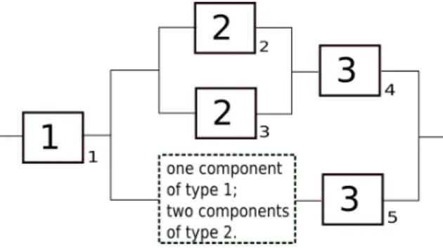
Figure 2: Bridge system with two types of components. The numbers inside the boxes indicate the component type. The numbers above the boxes indicate the component indices.

Table 1: Survival signature of the bridge system of Figure 2

l1 l2 (l1, l2) 0 [0,1,2,3] 0 [1,2] [0,1] 0 1 2 1/9 1 3 1/3 2 2 4/9 2 3 2/3 3 [0,1,2,3] 1 where D(Ck(t) =lk) =P(Ck(t)lk) P(Ck(t)lk 1). (8) 4. Numerical Examples

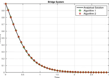
4.1. Bridge system with not repairable components

The purpose of this numerical example is to verify the proposed algorithms since for this simple problem analytical solutions are available. The system con-figuration is represented in Figure 2 , k= 1,2. The bridge system comprises of

325

six components, which belonging to two types. It has no series section or parallel section which can enable simplification. The survival signature can easily be com-puted either manually or using the R-packageReliabilityTheory[19]. The values of the survival signature are reported in Table 1 wherel1andl2indicate the number

of working component of type k = 1 and k = 2, respectively and (l1, l2) is the 330

survival signature of the bridge system. In this example the failure times of both component type 1 and 2 are obeying to exponential distributions with parameters

1 = 0.8 and 2 = 1.5, respectively, i.e. the components have a constant mean

time to fail. It is also assumed that the component once failed can not be repaired. The survival function of the bridge system is then calculated by means of the Algorithms 1 and 2. The resulting functions are then compared with the analytical

(14)

Time 0 0.5 1 1.5 2 2.5 3 Reliability 0 0.1 0.2 0.3 0.4 0.5 0.6 0.7 0.8 0.9 1 Bridge System Analytical Solution Algorithm 1 Algorithm 2

Figure 3: Survival function of the bridge system calculated by two simulation methods and analytical method, respectively.

solution. The survival function can be obtained from Equations (3) and (2):

P(TS > t) = 3 X l1=0 3 X l2=0 (l1, l2) ✓₃ l1 ◆ [1 e 0.8t]3 l1_[_e 0.8t_]l1 ⇥ ✓₃ l2 ◆ [1 e 1.5t]3 l2_[_e 1.5t_]l2 ₍₉₎

The results of the reliability analysis are shown in Figure 3, which shows a perfect

335

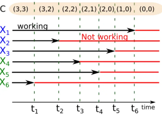
agreement of the simulation methods with the analytical solution. The Monte Carlo simulation has been performed usingN = 5000 samples and a discretisation timedt= 0.0015. The discretization time is only required to collect the numerical results (i.e. survival function) although the simulation of the system is continuous with respect to the time. Figure 4 shows an example of system evolution as a

340

function of time with associate number of working component Ck. In order to show the efficiency of the proposed algorithm, the evolution of the variance of the estimators as a function of number of samples has been computed and shown in Figure 5. Algorithm 2 shows a smaller variance compared to Algorithm 1, in particular when small sample sizes are used.

345

The bridge system is also analysed in presence of imprecision on the parameters of the failure distribution time. In this case it is assumed that the parameters of the component failure time are not known precisely. The bounds of the parameter distributions are 1= [0.4, 1.2] and 2 = [1.3, 2.1]. The bounds of the survival

functions are computed by means of the Algorithms 1 and 2. Since this system

Figure 5: Variance of the estimator of the survival function.

is a coherent system, only two numerical simulations are required, i.e. the lower bound of the survival function is computed using the lower bounds of the param-eter distribution and the upper bound is obtained adopting the upper bounds of the paramters 1and 2. The results are then compared to the analytical solution

adopting the method presented in [9]. The results of the simulation have been

fur-355

ther verified by estimating the survival function adopting a double loop approach. The double loop sampling involves two layers of sampling: the outer loop, called the parameter loop, samples values from the set of distribution parameters; while the inner loop computes the survival function stating for the system knowing the precise probability distribution functions. Then, the lower and upper bounds of

360

the survival function have been computed at each time of interest. The double loop Monte Carlo analysis has been performed using N = 5000 samples for the

(16)

0 0.5 1 1.5 2 2.5 3 0 0.1 0.2 0.3 0.4 0.5 0.6 0.7 0.8 0.9 1 Time Reliability

Bridge System with parameter imprecision

Analytical Solution (Lower Bound) Analytical Solution (Upper Bound) Simulation Extreme (Lower Bound) Simulation Extreme (Upper Bound) Double Loop (Lower Bound) Double Loop (Upper Bound)

Figure 6: Bounds of the survival function of the bridge system calculated by means of the Algo-rithm 1 and 2 using bounds of the distribution parameter (Simulation Extreme) and compared with analytical solutions and the double loop approach.

inner loop and 1000 samples for the parameter loop. The results are collected in a counter using a discretisation time stepdt= 0.0015.

The results of the simulation considering imprecision are reported in Figure 6

365

showing a perfect agreement with the analytical solutions.

4.2. Bridge system with repairable components

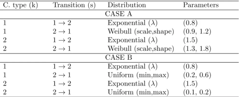
In this example the components of the bridge system shown in Figure 2 are considered repairable. Hence, the components can be in two di↵erent states: work-ing (s= 1) and not-working (s= 2). Two cases are analysed considering di↵erent

370

distributions for the repair times as shown in Table 2. Analytical solutions are Table 2: Parameters of repairable components in the bridge system. State 1: Working, State 2: Not-working.

C. type (k) Transition (s) Distribution Parameters CASE A 1 1_!2 Exponential ( ) (0.8) 1 2_!1 Weibull (scale,shape) (0.9, 1.2) 2 1!2 Exponential ( ) (1.5) 2 2!1 Weibull (scale,shape) (1.3, 1.8) CASE B 1 1!2 Exponential ( ) (0.8) 1 2!1 Uniform (min,max) (0.2, 0.6) 2 1!2 Exponential ( ) (1.5) 2 2!1 Uniform (min,max) (0.1, 0.2)

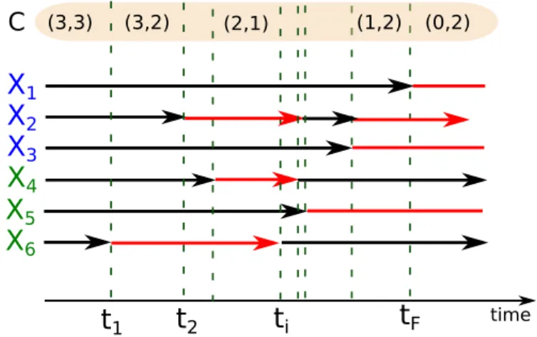
not available for analysing repairable systems and the system can only be analysed by adopting simulation methods such as the Algorithm 3. The estimated survival functionP(TS > t) is shown in Figures 8 and 10 for the CASE A and B,

(17)

respec-tively. An example of the evolution of the system is represented in Figure 7. The

375

0 0.5 1 1.5 2 2.5 3 Time 0.2 0.3 0.4 0.5 0.6 0.7 0.8 0.9 1 Reliability

Bridge System with repairable components: CASE A

Survival Signature Structure Function

Figure 8: CASE A: Survival function of the bridge system with repairable components calculated by means of the Algorithm 3 and a simulation method based on structure function.

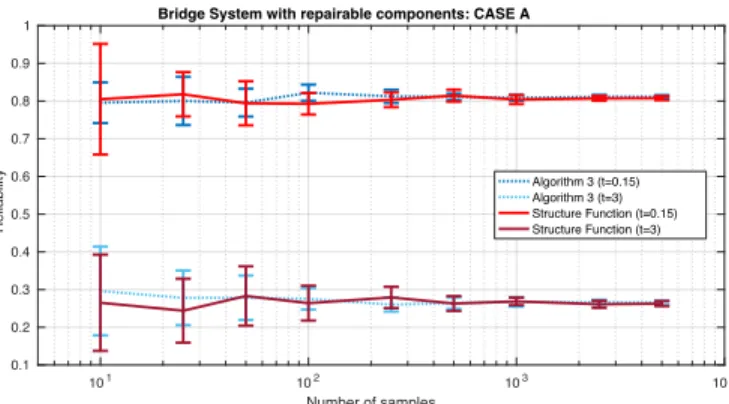
It is important to notice that the proposed approach (Algorithm 3) does not require the introduction of additional component types to analyse a system with repairable components. In order to verify the correctness of Algorithm 3 which

380

is based on survival signature, the results have been compared with the solution of simulation method based on the structural function. The minimum path sets of the Bridge system shown in Figure 2 are [1,2,3], [1,2,5,6], [1,3,4,5] and [1,4,6]. N = 5000 samples have been used to estimate the reliability of the system and the results shown in Figures 8 and 10 are in perfect agreement with the results obtained

385

(18)

101 ₁₀2 ₁₀3 ₁₀4 Number of samples 0.1 0.2 0.3 0.4 0.5 0.6 0.7 0.8 0.9 1 Reliability

Bridge System with repairable components: CASE A

Algorithm 3 (t=0.15) Algorithm 3 (t=3) Structure Function (t=0.15) Structure Function (t=3)

Figure 9: CASE A: Variance of the estimator for the bridge system with repairable components calculated by means of the Algorithm 3 and a simulation method based on structure function.

0 1 2 3 4 5 Time 0.5 0.6 0.7 0.8 0.9 1 Reliability

Bridge System with repairable components: CASE B

Survival Signature Structure Function

Figure 10: CASE B: Survival function of the bridge system with repairable components calculated by means of the Algorithm 3 and a simulation method based on structure function.

function of the number of samples adopting the Algorithm 3 based on survival signature and Monte Carlo method based on structural function.

4.3. Grey System

In order to illustrate the efficiency and the applicability of the proposed

sim-390

ulation approaches a complex system composed by 8 components of 5 types is analysed. The component failure types and distribution parameters are shown in Table 3, again a↵ected by imprecision. In addition, it is assumed that the exact configuration of part of the system is unknown as shown in Figure 12, i.e. it might be composed by an additional component of type 1 or two components of type 2

395

connected in parallel. However, the system can still be described using the sur-vival signature although a↵ected by imprecision [6]. This has the advantages of more realistic reflections of uncertainty on system functioning and the proposed

(19)

101 102 103 104 Number of samples 0.5 0.6 0.7 0.8 0.9 Reliability

Bridge System with repairble components: CASE B

Algorithm 3(t=0.15) Algorithm 3(t=3) Structure Function(t=0.15) Structure Function(t=3)

Figure 11: CASE B: Variance of the estimator with repairable components calculated by means of the Algorithm 3 and a simulation method based on structure function.

Figure 12: Grey system composed by eight components of 5 types with imprecision of the exact system configuration.

simulation methods are also directly applicable . Table B.7 shows the imprecise structural signature. For instance, if 2 components of type 1 and 1 component of

400

type 3 are working the system can be either in a failing state or working with a probability of 0.5 (if the unknown part of the system is composed by an additional component of type 1). Since the system in Figure 12 is a coherent system, Al-gorithm 2 is used to estimated the bounds of the survival function by collecting the bound values (i.e. intervals) of the survival signature during the Monte Carlo

405

simulation. In other words, the failure times of the components are sampled using the bounds of the failure time distribution as shown in the previous Section. In addition, in the Step 5’ of Algorithm 2, the values of the survival signatures ti

and ti are evaluated and in the Step 6’ their values collected in two counters

V r(t) =V r(t) + ti andV r(j) =V r(j) + ti,8j:j·dt < ti. Hence, no additional 410

Monte Carlo simulation are required to estimate the bounds of the survival func-tion (the system reliability). If the component failure times are not a↵ected by

(20)

Table 3: Components failure types and distribution parameters for system of Fig.12 Component type Distribution Parameters

1 Weibull (scale,shape) ([1.6, 1.8],[3.3, 3.9]) 2 Exponential ( ) ([2.1, 2.5]) 3 Weibull (scale,shape) ([3.1, 3.3],[2.3, 2.7]) Time 0 0.2 0.4 0.6 0.8 1 1.2 Reliability 0 0.2 0.4 0.6 0.8 1 Lower Bound Upper Bound

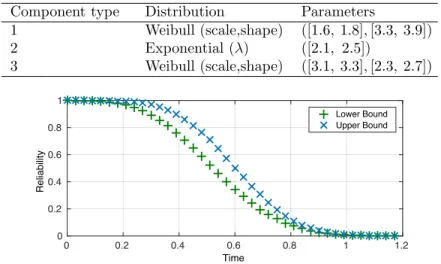
Figure 13: Upper and lower bounds of survival function for the system in Fig 12.

imprecision, only one Monte Carlo simulation would have been required to analyse the system with imprecision in the survival signature. In principle, Algorithm 1 can also be used for the estimation of the reliability bounds although it requires

415

some modifications in the sampling of the system status.

The upper and lower bounds of survival function for the system with impreci-sion both in the survival signature and on the component distribution parameters are shown in Figure 13. The simulations have been performed using 5000 sam-ples. This example shows the flexibility and the applicability of the simulation

420

approaches proposed for the analysing of a systems a↵ected by imprecision where no analytical solutions are available.

4.4. Complex System

In order to illustrate the efficiency and the applicability of the proposed simu-lation approaches, a complex system composed by 14 repairable components of 6

425

di↵erent types is analysed. The reliability block diagram of the system is shown in Figure 14 and the parameters of the components are reported in Table 4. The survival signature of this system can be referred in Appendix B.

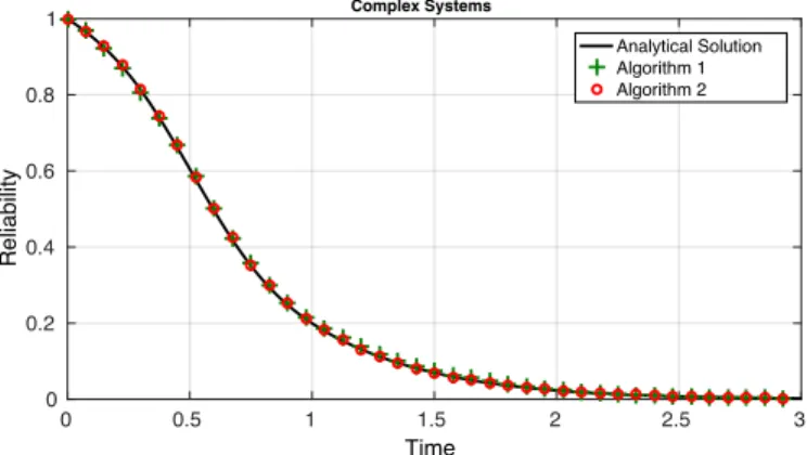
First, the system is analysed without considering the repairs (i.e. transition 2 ! 1 is not allowed). Hence, the reliability of the system can be estimated

430

adopting the proposed Algorithms 1 and 2. The results are shown in Figure 15 and Figure 16 for the case of non-repairable components with precise parameters and with imprecise parameters, respectively.

(21)

tran-Figure 14: Reliability block diagram of the 16 component system. 0 0.5 1 1.5 2 2.5 3 Time 0 0.2 0.4 0.6 0.8 1 Reliability Complex Systems Analytical Solution Algorithm 1 Algorithm 2

Figure 15: Survival function of the complex system calculated by Algorithms 1 and 2 and com-pared with analytical solution

.

sition, Algorithm 3 needs to be used. The proposed approach is generally

applica-435

ble and allows to estimate the reliability of complex system based on the survival function. Figure 17 shows the survival function for the case of repairable compo-nents. The black line shows the results when the parameters of the failure and repair distributions are precisely known.

When imprecisions are considered within repairable system, the bounds of the

440

survival function can be estimated by means of only two simulations as shown in Figure 6. These analyses require the calculation of the cumulative distribution function (CDF) bounds for component failure and repair, which are expressed as [F , F] and [R, R] respectively. Then, the lower bound of the survival function is estimated by considering the upper bound of the failure distributions and the

445

lower bound for the repair distributions (F , R) while the upper bound is obtained adopting the lower bound for the failure distribution and the upper bound for the repair distribution (F , R). The interval of the survival function can be seen in Figure 17.

(22)

0 0.5 1 1.5 2 2.5 3 3.5 Time 0 0.2 0.4 0.6 0.8 1 Reliability

Complex Systems with Parameter Imprecision

Simulation Extreme (Lower Bound) Simulation Extreme (Upper Bound) Double Loop (Lower Bound) Double Loop (Upper Bound)

Figure 16: Bounds of survival function of the system with imprecision.

0 5 10 15 20 Time 0 0.2 0.4 0.6 0.8 1 Reliability

Complex system with repairable components and imprecision

Upper Bound Lower Bound Precise

Figure 17: Survival function of the repairable complex system with imprecise and precise param-eters, respectively.

(23)

Table 4: Components failure (transition 1 !2) and repair (transition 2 ! 1) data for each component type of the complex system.

Component Transition Distribution Precise Imprecise

type (k) (s) parameters parameters

1 1_!2 Exponential ( ) (2.3) ([2.1, 2.5]) 1 2_!1 Uniform (min,max) (0.4, 0.6) ([0.3, 0.5], [0.5, 0.7]) 2 1_!2 Exponential ( ) (1.2) ([0.9, 1.4]) 2 2_!1 Uniform (min,max) (0.9, 1.1) ([0.8, 1.0], [1.0,1.2]) 3 1!2 Weibull (scale,shape) (1.7, 3.6) ([1.6, 1.8], [3.3, 3.9]) 3 2!1 Uniform (0.6, 0.8) ([0.5, 0.7], [0.7, 0.9]) 4 1!2 Lognormal (µ, ) (1.5, 2.6) ([1.3, 1.8], [2.3, 2.9]) 4 2_!1 Uniform (min,max) (1.0, 1.2) ([0.9, 1.1], [1.1, 1.3]) 5 1_!2 Weibull (scale,shape) (3.2, 2.5) ([3.1, 3.3], [2.3, 2.7]) 5 2_!1 Uniform (min,max) (1.2, 1.4) ([1.1, 1.3], [1.3, 1.5]) 6 1_!2 Gamma (scale,shape) (3.1, 1.5) ([2.9, 3.3], [1.3, 1.8]) 6 2_!1 Uniform (min,max) (1.1, 1.3) ([1.0, 1.2], [1.2, 1.4])

In terms of computational e↵ort of the analysis, the calculation of the survival

450

signature of the complex system using the R-package ReliabilityTheory requires only a few seconds on a common desktop computer.

The performance for very large numbers of components is an important topic for future research where it is important to separate computation of survival sig-nature from the simulation of the system. The first part can already be done

455

for quite substantial systems using the approach proposed in [10, 34] but which remains also a topic for research. The simulation of the system given the survival signature is almost independent on the number of components. In fact, the only parts of the simulation approach that scale with the number of components are the Steps 1 and 2 of the algorithm. In these steps the failure time of components

460

is sampled and then sorted. However, the computational cost of this part is negli-gible (fraction of seconds) up to million of components as shown in Figure 18. The figure shows the computational cost of sampling the failure time of components

(24)

102 104 106 108 Number of components 10-6 10-4 10-2 100 102 Computational Time [s] Step 1 Step 2 Step 1+2

Figure 18: Scalability of the simulation algorithm with respect the number of components (Steps 1 and 2 only).

from exponential distribution (Step 1 of the Algorithm) and then sorting all the sampled times (Step 2). Steps 3-7 depend on the reliability of the components

465

and the time of interest (Tf) and scale linearly with the number of failures

oc-curring before the time of interest. Clearly the total simulation time depends on the number of samples used. For the examples presented, the proposedsimulation methods allow to estimate the survival function in less than 20 seconds using 5000 samples on a common desktop.

470

5. Conclusions

The survival signature has been shown to be a practical method for performing reliability analysis of complex systems with multiple component types. However, analytical methods are applicable only in few cases or adopting di↵erent levels of simplifications and assumptions.

475

In this paper, efficient simulation methods have been proposed for system relia-bility analysis. The methods proposed are based on survival signature, which need to be computed only once making the analysis very efficient. The proposed simula-tion methods are generally applicable and they can be used to analyse realistic and complex systems with non-repairable and repairable components. Recently, a case

480

has been made for allowing the structure function for system reliability to be a, possibly imprecise, probability instead of a deterministic binary function [6]. This has advantages of more realistic reflections of uncertainty on system functioning and opens many interesting research questions. Such more general probabilistic structure functions can also be used in the survival signature in a straightforward

(25)

manner, hence the simulation methods presented in this paper can also directly be applied.

The feasibility and e↵ectiveness of the presented approaches have been illus-trated with two numerical examples, the results indicate that simulation methods based on survival signature are efficient for analysing reliability on complex

sys-490

tems.

Acknowledgement

This work was partially supported by the UK Engineering and Physical Sci-ences Research Council (EPSRC) grant EP/M018709/1.

Geng Feng would like to thank the support of China Scholarship Council.

495

Appendix A. Algorithms

The Algorithms 1-3 of the proposed methods are shown in this appendix. In the Algorithms the letter V is used to represent vectors while the letter M represents matrices. The symbol⇠

is used represents sampling from given distribution.

Appendix B. Survival Signature

500

The tables in this appendix show the survival signature of the complex system of Figure 14. The rows with survival signature values equal to either 1 or 0 have been omitted.

(26)

Algorithm 1

Require: N: Num. of simulations; dt: Discretisation time; Fk: CDF failure times, V c= [m1, m2, . . . , mk]: Number of components per type; N tnumber of

discretisation steps,

Set Vr(1:Nt)=0 .Initialise counter

Set C=sum(Vc) . Compute total number of components Set = Survival signature . Compute the survival signature

forn= 1 :N do . loop over number of samples

fork= 1 :Kdo .loop over number of component type

forj= 1 :mk do .loop over number of components M f(j, k)_⇠Fk .Sample failure time componentj of typek

end for end for

[V t, V i] =sort(M f) . Reorder transition times (V t) . Return component index vector (V i)

Old = 1 . Initialize variables

form= 1 :C do .loop over number of components V c(V i(m)) =V c(V i(m)) 1 .Update number working components

N ow= (V c) q N ow/ Old

if rand(1)< q then . system working

Old = N ew

else

for allj:j_·dt < V i(m)do

V r(m) =V r(m) + 1 .Update counter

end for

Break .Process next sample

end if end for

V r=V r/N . Normalise counter

(27)

Algorithm 2

Set C=sum(Vc) . Compute total number of components Set = Survival signature . Compute the survival signature

fork= 1 :Kdo .loop over number of component type

forj= 1 :mk do .loop over number of components M f(j, k)⇠Fk .Sample failure time componentj of typek

end for end for

[V t, V i] =sort(M f) . Reorder transition times (V t) . Return component index vector (V i)

z= 1 . Initialize index

form= 1 :C do .loop over number of components V c(V i(m)) =V c(V i(m)) 1 .Update number working components

whilez_·dt_V t(m)do V r(z) =V r(z) + (V c) .Update counter z=z+ 1 .Update index end while end for V r=V r/N . Normalise counter end for

(28)

Algorithm 3

Set C=sum(Vc) . Compute total number of components Set = Survival signature . Compute the survival signature Set Vs = Initial component Status .System initial conditions

fori= 1 :Cdo .loop over number of components V t(i)_⇠Fkl . Sample transition time componentz of typekin statel

end for

u = 1 .Initialise counter

whilemin(V t)_N t_⇤dt do

[tz, z] =min(V t) . Identify first system transitiontz . and corresponding component indexz Identify component typekof the componentz

whileu·dtV j do

V r(u) =V r(u) + (V k) .Update counter

u u+ 1 .Update index

end while

if V s(z) is working then

V c(k) =V c(k) 1 . Update component counter SetV s(z) NOT working .Update component status

else

V c(k) =V c(k) + 1 . Update component counter SetV s(z) working .Update component status

end if

SetV t(z)_⇠Fkl .Sample new transition time componentz . of typekin the statel=V j(z)

end while end for

(29)

Table B.5: Survival signature of a complex system in Figure 14; rows with (l1, l2, l3, l4, l5, l6) = 0 and (l1, l2, l3, l4, l5, l6) = 1 are omitted

l1 l2 l3 l4 l5 l6 (l1, l2, l3, l4, l5, l6) 3 1 0 [0,1] [0,1] 1 1/20 3 1 0 1 1 0 1/20 3 1 1 0 [0,1] 1 1/20 3 1 1 1 0 1 1/20 3 1 2 [0,1] 0 1 1/20 3 1 2 0 1 0 1/20 3 1 1 [0,1] 1 1 1/10 3 1 1 1 1 0 1/10 3 1 2 0 1 1 1/10 3 1 2 1 1 [0,1] 1/10 3 2 0 0 [0,1] 1 1/10 3 2 0 1 0 1 1/10 3 2 0 1 1 [0,1] 1/10 3 2 1 [0,1] 0 1 1/10 3 2 1 0 1 0 1/10 3 2 2 [0,1] 0 1 1/10 3 2 2 0 1 0 1/10 3 3 0 [0,1] [0,1] 1 3/20 3 3 0 1 1 0 3/20 3 3 [1,2] [0,1] 0 1 3/20 3 3 1 0 1 0 3/20 3 3 2 0 1 0 3/20 3 4 0 [0,1] [0,1] 1 1/5 3 4 0 1 1 0 1/5 3 4 [1,2] [0,1] 0 1 1/5 3 4 1 0 1 0 1/5 3 4 2 0 1 0 1/5 4 1 0 [0,1] [0,1] 1 1/5

(30)

l1 l2 l3 l4 l5 l6 (l1, l2, l3, l4, l5, l6) 4 1 0 1 1 0 1/5 4 1 [1,2] [0,1] 0 1 1/5 4 1 1 0 1 0 1/5 4 1 2 0 1 0 1/5 3 2 [1,2] [0,1] 1 1 4/15 3 2 1 1 1 0 4/15 3 2 2 1 1 0 4/15 4 2 [0,1,2] [0,1] 0 1 11/30 4 2 0 0 1 1 11/30 4 2 0 1 1 [0,1] 11/30 4 2 1 0 1 0 11/30 4 2 2 0 1 0 11/30 3 [3,4] 1 [0,1] 1 1 2/5 3 3 1 1 1 0 2/5 3 3 2 0 1 1 2/5 3 3 2 1 1 [0,1] 2/5 3 4 1 1 1 0 2/5 3 4 2 [0,1] 1 1 2/5 3 4 2 1 1 0 2/5 4 1 [1,2] [0,1] 1 1 2/5 4 1 [1,2] 1 1 0 2/5 4 3 0 [0,1] [0,1] 1 1/2 4 3 0 1 1 0 1/2 4 3 [1,2] [0,1] 0 1 1/2 4 3 1 0 1 0 1/2 4 3 2 0 1 0 1/2 5 1 0 [0,1] [0,1] 1 1/2 5 1 0 1 1 0 1/2

(31)

Table B.7: Imprecise survival signature of the system of Fig.12, (l1, l2, l3) = 0 and (l1, l2, l3) = 1 for both lower and upper bounds are omitted.

l1 l2 l3 [ (l1, l2, l3)] 1 1 1 [1/8,1/8] 1 1 2 [1/4,1/4] 1 2 1 [1/5,1/4] 1 2 2 [3/7,1/2] 1 3 1 [1/4,3/8] 1 3 2 [1/2,1/2] 1 4 1 [1/4,1/2] 1 4 2 [1/2,1/2] 2 0 1 [0,1/2] 2 0 2 [0,1] 2 1 1 [1/4,3/4] 2 1 2 [1/2,1] 2 2 1 [1/2,1] 2 3 1 [3/4,1]

l1 l2 l3 l4 l5 l6 (l1, l2, l3, l4, l5, l6) 5 1 [1,2] [0,1] 0 1 1/2 5 1 1 0 1 0 1/2 5 1 2 0 1 0 1/2 4 4 0 [0,1] [0,1] 1 3/5 4 4 0 1 1 0 3/5 4 4 [1,2] [0,1] 0 1 3/5 4 4 1 0 1 0 3/5 4 4 2 0 1 0 3/5 4 2 [1,2] [0,1] 1 1 2/3 4 2 1 1 1 0 2/3 4 2 2 1 1 0 2/3 4 3 [1,2] [0,1] 1 1 4/5 4 3 1 1 1 0 4/5 4 3 2 1 1 0 4/5 4 4 [1,2] [0,1] 1 1 4/5 4 4 1 1 1 0 4/5 4 4 2 1 1 0 4/5 5 2 0 [0,1] [0,1] 1 5/6 5 2 0 1 1 0 5/6 5 2 [1,2] [0,1] 0 1 5/6 5 2 [1,2] 0 1 0 5/6

(32)

References

[1] K. Kolowrocki, B. Kwiatuszewska-Sarnecka, Reliability and risk analysis of large systems with ageing components, Reliability Engineering & System

505

Safety 93 (12) (2008) 1821–1829.

[2] M. Modarres, What every engineer should know about reliability and risk analysis, Vol. 30, CRC Press, 1992.

[3] F. J. Samaniego, System signatures and their applications in engineering re-liability, Vol. 110, Springer Science & Business Media, 2007.

510

[4] S. Eryilmaz, Review of recent advances in reliability of consecutive k-out-of-n and related systems, Proceedings of the Institution of Mechanical Engineers, Part O: Journal of Risk and Reliability 224 (3) (2010) 225–237.

[5] F. P.A. Coolen, T. Coolen-Maturi, Generalizing the signature to systems with multiple types of components, in: Complex Systems and Dependability,

515

Springer, 2012, pp. 115–130.

[6] F. P. Coolen, T. Coolen-Maturi, The structure function for system reliabil-ity as predictive (imprecise) probabilreliabil-ity., Reliabilreliabil-ity Engineering and System Safety (154) (2016) 180–187.

[7] F. P.A. Coolen, T. Coolen-Maturi, A. H. Al-Nefaiee, Nonparametric

predic-520

tive inference for system reliability using the survival signature, Proceedings of the Institution of Mechanical Engineers, Part O: Journal of Risk and Re-liability 228 (5) (2014) 437–448.

[8] L. J.M. Aslett, F. P.A. Coolen, S. P. Wilson, Bayesian inference for reliability of systems and networks using the survival signature, Risk Analysis 35 (3)

525

(2015) 1640–1651.

[9] G. Feng, E. Patelli, M. Beer, F. P. Coolen, Imprecise system reliability and component importance based on survival signature, Reliability Engineering & System Safety 150 (2016) 116–125.

[10] S. Reed, An efficient algorithm for exact computation of system and survival

530

signatures using binary decision diagrams, Reliability Engineering & System Safety 165 (2017) 257–267. doi:10.1016/j.ress.2017.03.036.

URLhttp://dx.doi.org/10.1016/j.ress.2017.03.036

[11] P. R. Adduri, R. C. Penmetsa, System reliability analysis for mixed uncertain variables, Structural Safety 31 (5) (2009) 375–382.

535

[12] T. Augustin, F. P.A. Coolen, G. de Cooman, M. C.M. Tro↵aes, Introduction to imprecise probabilities, John Wiley & Sons, 2014.

[13] J. Butler, J. Jia, J. Dyer, Simulation techniques for the sensitivity analysis of multi-criteria decision models, European Journal of Operational Research 103 (3) (1997) 531–546.

540

[14] R. Y. Rubinstein, Optimization of computer simulation models with rare events, European Journal of Operational Research 99 (1) (1997) 89–112. [15] S. H. Zanakis, A. Solomon, N. Wishart, S. Dublish, Multi-attribute decision

making: A simulation comparison of select methods, European journal of operational research 107 (3) (1998) 507–529.

545

[16] E. Zio, P. Baraldi, E. Patelli, Assessment of the availability of an o↵shore in-stallation by monte carlo simulation, International Journal of Pressure Vessels and Piping 83 (4) (2006) 312–320.

(33)

[17] H. George-Williams, E. Patelli, A hybrid load flow and event driven simulation approach to multi-state system reliability evaluation, Reliability Engineering

550

& System Safety 152 (2016) 351367. doi:10.1016/j.ress.2016.04.002. [18] J. Song, W.-H. Kang, System reliability and sensitivity under statistical

de-pendence by matrix-based system reliability method, Structural Safety 31 (2) (2009) 148 – 156, risk Acceptance and Risk Communication, Risk Acceptance and Risk Communication. doi:DOI:10.1016/j.strusafe.2008.06.012.

555

URL http://www.sciencedirect.com/science/article/

B6V54-4T6KF7K-2/2/a3c60ec860317e6a429b905d0f00f69c

[19] L. J.M. Aslett, Reliabilitytheory: Tools for structural reliability analysis. r package (2012).

URLwww.louisaslett.com

560

[20] L. J.M. Aslett, MCMC for inference on phase-type and masked system lifetime models, Ph.D. thesis, Trinity College Dublin (2012).

[21] E. Patelli, Handbook of Uncertainty Quantification, Springer International Publishing, Cham, 2016, Ch. COSSAN: A Multidisciplinary Software Suite for Uncertainty Quantification and Risk Management, pp. 1–69. doi:10.

565

1007/978-3-319-11259-6_59-1.

URLhttp://dx.doi.org/10.1007/978-3-319-11259-6_59-1

[22] E. Patelli, M. Broggi, M. de Angelis, M. Beer, OpenCossan: An efficient open tool for dealing with epistemic and aleatory uncertainties, in: Vulnerability, Uncertainty, and Risk Quantification, Mitigation, and Management, ASCE,

570

2014, pp. 2564–2573.

[23] M. Marseguerra, E. Zio, Basics of the Monte Carlo Method with Application to System Reliability, LiLoLe Publishing, Hagen/Germany, 2002, iSBN: 3-934447-06-6.

[24] D. A. Alvarez, Infinite random sets and applications in uncertainty

anal-575

ysis, Ph.D. thesis, Arbeitsbereich f¨ur Technische Mathematik am Institut fr Grundlagen der Bauingenieurwissenschaften. Leopold-Franzens-Universit¨at Innsbruck, Innsbruck, Austria, available at https://sites.google.com/ site/diegoandresalvarezmarin/RSthesis.pdf(2007).

[25] B. M¨oller, M. Beer, Fuzzy-randomness - uncertainty in civil engineering and

580

computational mechanics, Springer-Verlag, 2004.

[26] M. Beer, S. Ferson, Imprecise probabilities-what can they add to engineering analyses?, Mechanical Systems and Signal Processing 37 (1-2) (2013) 1 – 3. [27] S. Ferson, V. Kreinovich, L. Ginzburg, D. S. Myers, K. Sentz, Constructing

probability boxes and Dempster-Shafer structures, Report SAND2002-4015,

585

Sandia National Laboratories, Albuquerque, NM, available athttp://www. ramas.com/unabridged.zip(January 2003).

[28] M. Beer, Y. Zhang, S. T. Quek, K. K. Phoon, Reliability analysis with scarce information: Comparing alternative approaches in a geotech-nical engineering context, Structural Safety 41 (0) (2013) 1 – 10.

590

doi:http://dx.doi.org/10.1016/j.strusafe.2012.10.003.

URL http://www.sciencedirect.com/science/article/pii/

S0167473012000689

(34)

Analy-sis, Society for Industrial and Applied Mathematics, Philadelphia, PA, USA,

595

2009.

[30] E. Patelli, D. A. Alvarez, M. Broggi, M. de Angelis, Uncertainty management in multidisciplinary design of critical safety systems, Journal of Aerospace Information Systems 12 (2015) 140–169. doi:10.2514/1.I010273.

[31] M. Beer, S. Ferson, V. Kreinovich, Imprecise probabilities in engineering

anal-600

yses, Mechanical systems and signal processing 37 (1) (2013) 4–29.

[32] L. V. Utkin, F. P. Coolen, Imprecise reliability: an introductory overview, in: Computational intelligence in reliability engineering, Springer, 2007, pp. 261–306.

[33] S. Ferson, C. A. Joslyn, J. C. Helton, W. L. Oberkampf, K. Sentz, Summary

605

from the epistemic uncertainty workshop: consensus amid diversity, Reliabil-ity Engineering & System Safety 85 (1) (2004) 355–369.

[34] G. Feng, S. Reed, E. Patelli, M. Beer, F. P. Coolen, Efficient reliability and uncertainty assessment on lifeline networks and imprecise survival signature, in: 2nd ECCOMAS Thematic Conference on Uncertainty Quantification in

610