Estimating Net Child Care Price Elasticities of Partnered Women With Pre-School Children Using a Discrete Structural Labour Supply-Child Care Model

The Australian National University

Centre for Economic Policy Research

DISCUSSION PAPER

ESTIMATING NET CHILD CARE PRICE

ELASTICITIES OF PARTNERED WOMEN WITH

PRE-SCHOOL CHILDREN USING A DISCRETE

STRUCTURAL LABOUR SUPPLY-CHILD CARE

MODEL

Robert Breunig

Australian National University

DISCUSSION PAPER NO. 653 November, 2011

ISSN: 1442-8636

O dd l an ds cap e h ead er

ES TIMATING NET CHILD CARE P RICE ELAS TICITIES OF P ARTNERED WOMEN WITH P RE-S CHOOL CHILDREN US ING A DIS CRETE S TRUCTURAL LABOUR S UP P LY-CHILD CARE MODEL

Xiaodong Gong and Robert Breunig 26 November 2011

ABS TRACT

Abstract: The purpose of this paper is to improve our understanding of the

relationship between child care price and women's labour supply. We specify and estimate a discrete, structural model of the joint household decision over women's labour supply and child care demand. Parents care about the well-being and development of their children and we capture this by including child care directly in household utility. Our model improves on previous papers in that we allow formal child care to be used for reasons other than freeing up time for mothers to work (such as child development) and we allow mothers’ work hours to exceed formal child care hours. As informal and paternal care are important features of the data, this second relaxation of previous hour constraints is particularly important. We estimate the model using data from 2005 to 2007 from the Household Income and Labour Dynamics in Australia (HILDA) Survey. We find that on average a one percent increase in the net price of child care leads to a decrease in hours of labour provided by partnered women of 0.10 per cent and a decrease in the employment rate of 0.06 per cent. These estimates are statistically significant. Furthermore, we find that labour supply responses are larger for women with lower wages, less education, and lower income.

JEL Classification Numbers: C15; C35; J22.

Keywords: Child care demand; child care price; women's labour supply; elasticities; discrete choice model

ACKNOWLEDGEMENTS: XIAODONG GONG IS AT THE NATIONAL CENTRE FOR SOCIAL AND ECONOMIC

MODELLING AT THE UNIVERSITY OF CANBERRA.ROBERT BREUNIG IS WITH THE RESEARCH SCHOOL OF ECONOMICS AT THE AUSTRALIAN NATIONAL.WE ARE GRATEFUL TO ANTHONY KING AND GORDON

LESLIE FOR COMMENTS ON AN EARLIER DRAFT OF THE PAPER. GUYONNE KALB AND STEPHAN

WHELAN COMMENTED ON A RELATED PAPER AND THEIR INSIGHTS ARE ALSO REFLECTED IN THIS PAPER. WE HAVE FURTHER BENEFITED FROM THE COMMENTS OF PARTICIPANTS AT THREE CONFERENCES WHERE WE PRESENTED THIS WORK IN JULY 2011: THE ECONOMETRIC SOCIETY

AUSTRALASIA MEETINGS IN ADELAIDE; THE AUSTRALIAN CONFERENCE OF ECONOMISTS IN

CANBERRA, AND THE HILDASURVEY "10TH ANNIVERSARY"RESEARCH CONFERENCE IN

MELBOURNE. ANY OMISSIONS AND MISTAKES ARE THE SOLE RESPONSIBILITY OF THE AUTHORS.

THIS PAPER USES UNIT RECORD DATA FROM THE HOUSEHOLD,INCOME AND LABOUR DYNAMICS IN

AUSTRALIA (HILDA)SURVEY.THE HILDAPROJECT WAS INITIATED AND IS FUNDED BY THE

AUSTRALIAN GOVERNMENT DEPARTMENT OF FAMILIES,HOUSING,COMMUNITY SERVICES AND

INDIGENOUS AFFAIRS (FAHCSIA) AND IS MANAGED BY THE MELBOURNE INSTITUTE OF APPLIED

ECONOMIC AND SOCIAL RESEARCH (MELBOURNE INSTITUTE).THE FINDINGS AND VIEWS REPORTED IN THIS PAPER, HOWEVER, ARE THOSE OF THE AUTHOR AND SHOULD NOT BE ATTRIBUTED TO EITHER

E

• In this paper, we specify and estimate a model for partnered women's simultaneous decisions about how much to work and how much child care to use.

• The model is an improvement over previous research in that it allows for comparison of alternative policies which affect household budget constraints, such as policies which change child care costs, and also allows for analysis of the distributional effects of such policies.

• The model is realistic in that labour supply and child care decisions are treated jointly and both hours worked and hours of child care demanded are chosen from a small set of commonly observed values. Hours can not be adjusted in arbitrarily small amounts but must respect the real-life constraints of the labour market and slots typically offered by child care providers.

• The model includes constraints which require that children be cared for at all times by someone other than the mother while the mother is working. Such constraints are important to avoid bias in the estimated effects of child care prices.

• The paper improves the modelling of the relationship between hours of child care and mothers’ working time in two important ways:

- The model allows for the use of child care for purposes other than freeing up mothers’ time to work. For example, child care may be used to improve children’s development.

- The model allows hours worked by the mother to exceed hours of formal child care, with the difference being made up by informal and/or paternal care. This relaxation of hours restrictions imposed in previous research is important in that we observe in the data that over thirty per cent of working mothers work more hours than the hours spent by their children in formal care.

Both of these innovations are novel in the literature.

• We model and include effects of the personal tax system and major transfer payments including New Start Allowance, Parenting Payment Partnered, Family Tax Benefits, and Child Care Benefit.1

• The model is estimated using data from Waves 5 through 7 (2005 – 2007) of the ‘in-confidence’ version of the Household Income and Labour Dynamics in Australia (HILDA) Survey.

• The model is estimated for partnered women with pre-school children. This homogeneous sample reduces model bias from unobserved factors. This reduction in bias comes at a cost, however, as the results may not be applicable to other groups (partnered women with school-aged children or single parents of pre-school children, for example).

1 We do not model fringe benefits tax which may be related to child care if it is received as part of a compensation package. We also do not model Child Care Rebate (CCR) which was introduced (as the then Child Care Tax Rebate) during our analysis period but which was initially paid to families with a long delay. We argue that CCR did not affect families' decisions about child care and in the prices we construct from the data provided by families it appears that they did not include CCR in their calculations.

• We focus on the estimation of net price elasticities, which provide an estimate of how labour supply or child care demand changes for a change in the net price of child care. The gross price is the posted price at a child care centre. The net price is what families actually pay out of pocket after accounting for any subsidies or rebates. Economic theory tells us that net, not gross, prices should determine behaviour. Government policy in Australia is targeted at changing the actual out-of-pocket costs that families face (rather than, for example, fixing prices) and thus the net price elasticity is more appropriate for understanding the effect of policy. The gap between the net and gross price elasticities is not constant across the population because of the means testing of subsidies. Net price elasticities are thus more useful to study the distributional effects of policy.

• We confirm the findings of Gong et al. (2010) that the labour supply behaviour of partnered women with young children responds (negatively) to child care price;

- we find that a one per cent increase in the net price of child care for pre-school children leads to a decrease in hours worked by partnered women of 0.10 per cent. Such a price change leads to a decrease in the employment rate of 0.06 per cent. These estimates are statistically different from zero.

- the analogous gross child care price elasticities are similar. A one per cent increase in the gross pre-school child care price causes mothers' hours of work to decrease by 0.11 per cent and mothers' employment rate to decrease by 0.07 per cent.

- both labour supply and child care demand are more responsive in families with lower income, with less educated parents, and with lower female wages. Poorer families, for whom child care expenses may take up a larger fraction of the household budget, are thus more affected by child care price changes than wealthier families. - Gong et al. (2010) found a gross child care price elasticity of

employment of -0.29. The gross child care price elasticity from the approach of Gong et al. (2010) for the sub-group of pre-school children as considered in this paper is -0.15, which is not statistically different than the corresponding point estimate of -0.07 presented in this paper. The differences in the two papers can be explained by five factors:

 the two papers estimate different models;

 the two papers use different methods to calculate elasticities;  the two papers use different samples;

 the price variable which is being changed in the elasticity calculation is different in the two papers; and

 we impose a quantity constraint, in this paper, that total child care hours (formal, informal and paternal) be at least as great as a mother’s working hours which allows hours of formal child care to exceed hours worked by the mother. There was no such constraint imposed in the previous paper.

- The last two points are the most important. Gong et al. (2010) look at the effect on women's labour supply of changing all child care prices whereas this paper only looks at changing the price of child care for pre-school children. Naturally changing more child care prices has a larger effect than changing fewer prices so it is not surprising that this paper reports a smaller elasticity. Regarding the quantity constraint, Duncan et al. (2001) showed that elasticities may be overestimated if quantity constraints are not taken into account.

O dd l an ds cap e h ead er

C

ONTENTS

2. MODEL AND ESTIMATION ... 4

2.1 The discrete choice model of labour supply and child care ... 4

2.1.1 More realistic labour and child care markets ... 5

2.1.2 Formal child care, informal child care and mother's working hours ... 6

2.1.3 Technical specification of the model ...10

2.2 Estimation ... 14

2.3 Simulations and the calculation of the net price elasticity ... 16

3. DATA ...17

3.1 Data source and sample ... 17

3.2 Child care price ... 22

4. RESULTS ...26

4.1 Estimation results ... 26

4.2 Simulation results ... 30

4.2.1 Labour supply elasticities ...31

4.2.2 Relationship to previous results ...31

4.2.3 Child care demand elasticities ...33

4.2.4 Elasticities of subsamples ...34

O dd l an ds cap e h ead er

ES TIMATING NET CHILD CARE P RICE ELAS TICITIES OF P ARTNERED WOMEN WITH P RE-S CHOOL CHILDREN US ING A DIS CRETE S TRUCTURAL LABOUR S UP P LY-CHILD CARE MODEL

Xia o d o n g Go n g a n d Ro b e rt Bre u n ig

1.

I

The purpose of this paper is to increase our understanding of the relationship between the price of child care and the labour supply behaviour of partnered women. Many governments, including Australia, subsidise child care to encourage female labour force participation and also to promote child development. A large part of the effectiveness of these subsidies thus depends crucially upon the labour supply responsiveness of women to child care costs. In this paper we build a model that can be used to understand and compare the labour supply effects of alternative tax and subsidy policies which affect child care prices.

In a previous paper, Gong et al. (2010) showed that there is a negative relationship between child care price and partnered women's labour supply. They showed that measurement error in child care price is a problem and they addressed the problem by constructing local area prices using detailed, child-level data. However, they used a linear labour supply model which does not correspond to the actual work choices which partnered women face. They also estimate their model in a way that embeds the current tax system and child care subsidy policies making the model inappropriate to use for evaluation of alternative policies. In this paper, we use their improved method of price construction but address these two limitations through a more realistic labour market model combined with an approach which can be used to evaluate competing policy proposals.

In this paper we focus on the estimation of the net price elasticity, which measures how labour supply or child care demand changes for a change in the

net price of child care. Gong et al. (2010) only provided estimates of gross price elasticities. The gross price is the posted price at a child care centre. The net price is what families actually pay out of pocket after accounting for any subsidies or rebates. It is this latter price that economic theory tells us should determine behaviour. Government policy on the cost of child care in Australia is targeted at changing the actual out-of-pocket child care costs that families face (rather than, for example, fixing prices) and thus the net price elasticity is more appropriate for understanding the effect of policy. It is important to note that the gap between the net and gross price elasticities is not constant across the population because of the means testing of subsidies. For some demographic groups, net and gross price elasticities may be quite similar whereas for others they may be quite different. Since we also care about the distributional effects of policy, this provides another argument for the importance of net price elasticities.

In order to estimate these net price elasticities, we specify and directly estimate the household's utility function. In this respect, our paper is similar to those of Blau and Robins (1988); Ribar (1992, 1995); Blau and Hagy (1998); Duncan et al. (2001); and Kornstad and Thoresen (2006, 2007). We construct and estimate a joint discrete structural model of labour supply and child care demand for partnered women with pre-school children.2

2 _{In this paper, partnered women with young children include married women and women in} de facto relationships. These women are also referred to as `mothers’ and their spouses/partners are referred to as `fathers’.

We focus on mothers with pre-school children because they are the group for whom the relationship between

labour supply and child care is strongest. We assume that women choose work hours and hours of formal child care from a small set of realistic values which reflect typical work hour patterns and typical time slots which are available through child care providers. The framework may be used to estimate the effects of policy changes which affect the household budget constraint, such as child care price subsidies, wage subsidies or cash transfers.

Our paper offers two important methodological innovations. First, to the best of our knowledge, this is the first paper that explicitly includes child care as an argument of the utility function of similar discrete choice models. Previous papers have incorporated child care into such models in very restrictive ways. Kalb and Doiron (2005) included child care costs in the budget constraint of a standard discrete labour supply model but child care did not enter the utility function. Kornstad and Thoresen (2006, 2007) allowed the possible labour supply choices to depend upon mode of child care but restricted the utility function to depend only upon leisure and consumption. Since parents derive utility from the well-being of their children and since child care can be an input into children's educational development, it is important to allow child care to enter the utility function.

Second, our modelling of the relationship between hours worked by the mother and hours of child care improves upon the previous literature by allowing formal

child care to be used for reasons other than allowing the mother to work and by accounting for the role of informal and paternal care in freeing up time for mothers to work. Children must be cared for at all times. Duncan et al. (2001) showed that it is important to constrain the number of child care hours to be at least as large as the hours of labour supplied by the mother. They showed that failure to do so can bias child care price effects. But Duncan et al. (2001) then

constrained the number of paid (or formal) child care hours to be greater than the number of hours worked by the mother, ignoring the possible contribution of paternal and informal care. Kornstad and Thoresen (2006, 2007) also impose an hours constraint, specifically that the mother’s work hours must be exactly equal to paid child care hours. In our view, this is too restrictive. We observe in the data (see below) that over thirty per cent of households use less hours of formal child care than the number of hours worked by the mothers. This clearly violates the constraints imposed by Duncan et al. (2001) or Kornstad and Thoresen (2006, 2007). Our model requires that the number of total child care hours (formal, informal and paternal) be at least as large as the number of hours worked by the mother. Formal child care hours may be greater or smaller than hours worked by the mother. Thus, our approach improves on both of these previous attempts to model quantity constraints.

The rest of the paper is organised as follows. In the next section (Section 2) we discuss the model, the estimation method, and the simulation approach we use to estimate elasticities. Section 3 describes the data. In Section 4, we present the estimation results of the model coefficients and the elasticities simulated from those estimates. This includes discussion of the relationship between the results in this paper and earlier results. Section 5 concludes.

2.

M

2.1

The discrete choice model of labour supply and child care

We estimate a discrete, structural model of the joint decision regarding hours of labour supplied by partnered women and household-level child care demand for families with pre-school children. The model assumes that households maximise their utility. Households get utility from consumption, leisure, and

child development. Households choose hours of work by the mother, taking into account the trade-off between additional consumption which is made possible by working more hours but reduced leisure and time with children. Hours of formal child care are chosen to maximise child development and to free up the mother's time for work, but must be paid for at the market rate. We first discuss two important innovations in our paper: restricting the set of possible hours of work and child care to more realistically reflect labour market and child care conditions; and the relationship between hours worked, hours of formal care, and hours of paternal and informal care. We then discuss the technical implementation of our model.

2.1.1 More realistic labour and child care markets

The theoretical framework in this paper assumes that the decision about whether or not to work and how many hours to work for partnered women is made simultaneously with the decision of whether or not to use child care and how much child care to use. Blau and Robins (1988); Blau and Hagy (1998); and Connelly (1992) pioneered this approach, but these early papers assumed that hours worked and hours of child care demanded adjusted exactly to families' desires. For example, a partnered woman could choose to work 36 hours and if a small change in circumstances made it preferable for her to work 36.5 hours, she could adjust her labour supply exactly.

Our model is based on the standard discrete neo-classic labour supply model first developed by Van Soest (1995), but extended to include maternal child care as an explicit argument of the household utility function and to define the budget constraint over a small, discrete set of possible working hours and formal child care hours rather than over working hours alone. For example, an individual may choose to work 35 or 40 hours, but not a value in between these

two points. (In practice, as described below, we allow eight different possibilities for working hours and six different possibilities for formal child care hours.) Families pick the combination of mother's working hours and formal child care that maximises their well-being from this set of 48 possible combinations of hours worked and hours of child care demanded. Kornstad and Thoresen (2007) estimate a similar model in that households are constrained in their choice of work and child care hours to a discrete set of points. However, our paper differs in the treatment of the relationship between formal child care and hours worked by the mother, as described below.

2.1.2 Formal child care, informal child care paternal care and mother's working hours

In our model, we assume the following:

(1) During waking hours, children are cared for in one of four possible ways: by the mother; by the father; in a paid, formal child care setting; or in an informal child care setting. This last category will include care by other relatives or friends and may be paid or unpaid.

(2) In our model, we combine the father’s time caring for children with informal care. This is partially driven by data restrictions. We do not observe hours or price of informal care. Nor do we observe hours of care by the father. In our model of the time allocation for mothers and children, therefore, these two types of care appear interchangeable. The model does allow for fathers to spend time taking care of children and allows the amount of time which fathers spend taking care of children to vary across households, but this care is not explicitly modelled.

(3) We assume that fathers’ hours worked do not respond to changes in the price of formal child care or to mothers’ wages. This is assumed for

tractability of the model but also corresponds to evidence that mothers still bear a disproportionate share of time in taking care of children (Sayer, 2005; Kalenkoski et al., 2005). Kalenkoski et al. (2005) also confirmed a common finding that while women's market work responds to the presence of children, men's market work does not. Kimmel and Connelly (2007) modelled women's time spent in a variety of activities including home production and childcare and similarly treated fathers’ behaviour as fixed.

(4) The household may choose to use formal child care regardless of whether the mother is at work or not. Formal care may exceed mother's working hours and may be used for purposes such as child development or freeing up time for the mother for activities other than paid work.

(5) We impose the restriction that total child care hours are at least as great as the hours of paid work by the mother and model informal and paternal child care as the difference between mother's working hours and formal child care hours. If formal child care hours equal or exceed mother's working hours, we assume that informal and paternal child care are zero. Otherwise, we set combined paternal and informal child care equal to mother's hours worked less hours in formal child care.3

3 _{An alternative approach would be to use reported hours of informal care and to} simultaneously model demand for formal and informal care alongside mother's labour supply. One immediate problem is that there is no information on price for informal care (in our data, only 10 per cent report paying for informal child care) even though families may incur non-pecuniary costs.

Families will face different costs and benefits of informal care depending upon the proximity of grandparents or other relatives or the presence of

other potential care-takers at home and we account for this in the model. Our approach is an improvement over Duncan et al. (2001) and Kornstad and Thoresen (2007) who assume, unrealistically, that formal child care hours must be greater than or equal to mother's hours of work. In our data, see below, about one-third of households report formal child care exceeding mother's working hours.

Figure 1 presents the household’s decision over the allocation of the child's time. Sleep (the darkest shaded area) is treated as fixed and the family decides over the allocation of the green parts--how to split the remaining time into care by the mother, formal child care and informal/paternal child care.

Figure 2 presents the mother's time allocation. After sleeping time, which is treated as fixed, mother's remaining time (the three most lightly shaded sections of Figure 2) is allocated between working, taking care of children, and leisure. Two `adding-up' constraints implied from (1) - (4) above must hold:

• Mother's time taking care of child = child's time being taken care of by mother

• Child's time in informal/paternal care = mother's working hours - child's time in formal care (or zero if this is negative)

We further assume that, for mothers with both pre-school and school–aged children, the primary consideration of the mother when she makes her labour supply and child care usage decisions is the well-being of the pre-school child(ren). That is, we assume that when school-aged children are present together with pre-school children in the same household, child care of the school-aged children outside school hours is assumed to mirror that of the pre-school children. Again, this is for tractability. For example, if formal hours of child care for the pre-school child are 40 and the school-age child is in school 30 hours per week then we assume that the school-age child is in before- and/or

Figure 1: Child's Time

Cared for by Mother Formal child care Informal/paternal child care

Figure 2: Mother's time

Sleep Leisure

Caring for children Working

after-school care for 10 (40 less 30) hours per week. We test this assumption in two ways. First, we replace this assumption with an assumption that formal child care of school-aged children is fixed and does not enter the utility function. Secondly, we estimate the model using households with pre-school children only. We present these results in the Appendix and discuss them in section 4.2.3. None of the conclusions of the paper are sensitive to this assumption.

2.1.3 Technical specification of the model

The household is assumed to maximise a trans-log utility function by choosing consumption

y

each of her K children (indexed by i) from a set of discrete options:

1

, , f , , fK ( ) ' ' , (log , log , log ) '

m m y h cMaxc U v =v Av+b v v≡ y l c (1) 0 1 s.t. ( , ) ( , ). K i fi i y τ y wh X ϕ p c X = ≤ + −

∑

y is general consumption net of child care costs which is determined through the budget constraint (2) by asset income and father’s income (both captured in

0

y ), the mother’s wage (w) and working hours, and the tax and transfer system

which is captured by the function τ and which depends upon household characteristics, X .4 The function captures child care subsidies which depend ϕ upon child care costs (price, which may vary by the age of the child, pi

multiplied by usage) and household characteristics. In addition to requiring that formal care of school-aged children be determined by the care needs of the

4 _Inτ _{, we include Newstart Allowance (NSA), Parenting Payment Partnered (PPP), Family Tax} Benefits A and B, together with personal income tax, Medicare levy, and Low Income Tax Offset (LITO). Tables 2 and 3 list the variables that are contained in X.

school children as described in 2.1.2 above, we also assume that all pre-school children use the same amount of formal care and pay the same price. This can be alternatively viewed as allowing differences in hours and price of care for pre-school children, but modelling the family's average demand.

m

l is the leisure of the mother which is specified as the difference between her

time endowment (Tm) and time spent either working or caring for children as in

Figure 2 above

l_m =T_m− −h c_m, (3)

m

c is the time spent on maternal care which is specified as

cm =min{Tc−h T, c−cf}, (4) where Tc is the time during which children need to be cared for either by the

mother, by the father, through the formal market or informally. Tc represents

the three most lightly shaded sections of Figure 1.

The parameters of the utility function are summarised in A, a symmetric 3 3×

parameter matrix with entries Aij, (i j, =1, 2, 3), and b=( ,b b b1 2, 3) ', a vector with

three parameters. b1 is a constant, but b2 and b3 are specified to allow both

observed and unobserved individual and household characteristics to affect utility:

𝑏𝑘 = ∑𝑆𝑠=1𝑘 𝛽𝑘𝑠𝑥𝑠𝑘 + 𝜀𝑝𝑘, (k=2,3) (5)

where 𝑥𝑠𝑘 are exogenous characteristics including the age of the mother and the

children, number of children in each age group, and other characteristics that describe the family composition such as the presence of extra female adults. In

the case of multiple children, maternal child care is measured as the average number of maternal care hours for all pre-school children in the household and the impact of the number of children on utility is through b3. That is, the number

of children affects the marginal utility of maternal care by shifting b3. (This

explains why b2 ≠b3 in equation (5) above. The k subscript on S allows for

different characteristics to enter the two equations.) Moreover, the potential impact of informal child care is also allowed for by the inclusion of a dummy in

3

b equal to one if h>c_f . This dummy controls for which condition in equation (4) determines maternal child care hours and equals one if the family makes recourse to informal child care (as calculated by our residual measure of informal child care usage). The error terms εpk may be interpreted as random preferences due to unobserved characteristics.

Working hours and formal child care hours may take the following values: {0,8,16, 24, 32, 40, 48,56} h∈ , (6) and {0,10, 20, 30, 40,50}, fi c ∈ (7) These can be chosen in any of the possible 48 combinations, allowing a wide range of part-time and half-day possibilities for both work and formal care. To estimate the model, we add random disturbances µj (as in Van Soest, 1995)

to each alternative in the choice set, as in the multinomial logit model (Maddala, 1983):

( , , ) ( 0,..., 48)

j j j mj mj j

where µj’s are independently and identically distributed with a type I extreme

value distribution, and are independent of all observable and unoberservable terms in the model.

The mother chooses alternative j if it is the alternative (out of m*g=48) from

which she derives the most utility, i.e. if Uj is the largest among all the

alternatives. Conditional upon εpk, _X , and w, the probability that _j is chosen is

, , , 1 exp( ( , )) Pr[ for all ] . exp( ( , )) j mj mj j i m g i mi mi i U y l c U U i U y l c ∗ = ≥ =

∑

logw=π'z+εw (10)

where z is a vector of individual characteristics of the mother. Her education level, current area of residence measured by capital city and state, and a variable equal to one if the mother lived with both of her parents when she was 14 (to capture stability while growing up) are included in the wage equation but not in the utility function and serve the role of exclusion restrictions. π is a vector of parameters to be estimated. εw is an unobserved term, assumed to be normally

distributed with mean zero, independent of z, but is allowed to be correlated with εpk.

As in similar models (for example, Gong and Van Soest, 2002), unobserved fixed benefit of not working (FB) is added to the income at zero hours of work. Thus

the utility of all alternatives at zero hours of work are replaced by 0 0, ( , _{m m}) U y +FB l c . FB is specified as ' FB=δ t (11)

where t is a vector of exogenous variables (which are listed in Table 2) and δ is

a vector of parameters. Positive fixed benefits increase the probability of not working by increasing the utility of non-participation. They can be interpreted equally as fixed costs associated with working.

2.2

Estimation

If all the wages were observed and there were no unobserved preferences, the model could be estimated by maximum likelihood with the likelihood contribution given by Equation (9). With unobserved wages, the wage Equation (10) also needs to be estimated. This is done simultaneously with the joint labour supply-child care model. With the presence of unobserved preferences in leisure and maternal child care, maximum likelihood estimation would require evaluation of the three-dimensional integral defined over the distribution of the error terms εw, εp2, and εp3. Numerical integration in more than two dimensions can be difficult to solve.

We use Simulated Maximum Likelihood (SML) to avoid this multi-dimensional numerical integration. Denoting the probability of working hj hours and using

j

c hours of formal child care conditional on εp2, εp3, and wage rate5 3 2 Pr_h=h c_j, _f =c_j | ,wε εp , p _ (j=1,..., 48), by (12)

5 Throughout, we condition on earnings of the husband, other non-labour income, child care price, and other exogenous explanatory variables. These are suppressed in our notation.

The exact likelihood contribution for someone observed to work h0 and use c0

hours of formal child care with observed gross wage rate w0 is then given by

3 3 3

2 2 2

0 0 0 1 0 2 0 0

Pr[ , _f | , p , p ] ( p | ) ( p | )d pd p ( ),

L=

∫∫

3 3 3

2 2 2

0 0 1 2

Pr[ , f | , p , p ] ( p | ) ( p | ) ( )d p d pd ,

L=

∫∫∫

(w)

f is the density of the wage rate (or of εw). The three error terms εw, εp2, and 3

p

ε are specified to follow a joint normal distribution of which the parameters are to be estimated: �𝜀 𝑤 𝜀𝑝2 𝜀𝑝3 � ~𝑁(0, Σ), where Σ= � 𝜎𝑤2 𝜎𝑤𝑝2 𝜎𝑤𝑝3 𝜎𝑤𝑝2 𝜎𝑝22 0 𝜎𝑤𝑝3 0 𝜎𝑝23 � (15) The numerical multi-dimensional integral is approximated by a simulated mean: for each individual, we take R draws from the distribution of the error terms (εw, εp2, and εp3) and compute the average of the _R likelihood values conditional on these draws. The integral Equation (13) is thus approximated by

3 2 0 0 0 0 1 1 Pr , | , , ( ), R p p f r r r L h h c c w f w R = ε ε   =

∑

And Equation (14) is replaced by 3 2 0 0 1 1 Pr , | , , , R p p f r r r r L h h c c w R = ε ε   =

∑

where logwr =π'z+εrw and ( w r ε , p2 r ε , p3 r

ε ) (r=1,..., )R are based upon draws from the distribution of (εw, εp2, εp3).

The draws are taken from Halton sequences using the procedure described in Train (2003). The estimator resulting from random independent draws is inconsistent for fixed R, but will be consistent as R tends to infinity with the number of observations of the sample.6

2.3

Simulations and the calculation of the net price elasticity

Many studies (see e.g., Morokoff and Caflisch, 1995, Sloan and Wozniakowski, 1998, Bhat, 2001, Train, 2003, Sandor and Train, 2004) show that using ‘quasi-random’ draws which are designed to provide better coverage than independent draws, simulation can be more efficient in terms of reduced simulation errors for a given number of draws. In particular, Bhat (2001), Train (2003), and Sandor and Train (2004) all tested Halton sequences for mixed logit models and found their use to be superior to random, independent draws.

Labour supply and child care demand behaviour of households may be described by their corresponding elasticities. Due to the complexity of the model, simulation is needed to derive elasticities and to estimate policy effects. When calculating the elasticities, hours of work and child care are calculated as `expected hours’, that is computed as a probability weighted sum of hours over all possible values which hours can take. Wage, gross child care price, and income elasticities for each observation are derived by increasing all wage rates, gross child care price, or other incomes by 1 per cent and calculating the percentage change of average expected hours or average expected employment rate. The net child care price elasticity is calculated as the ratio between the gross price elasticity and the percentage change in the net child care price

6 _{If n R/} →_{0 and with independent drawings across observations, the method is} asymptotically equivalent to maximum likelihood (see Lee, 1992, or Gourieroux and Monfort, 1993 for references).

corresponding to a 1 per cent change in the gross child care price. From these, we calculate the average elasticities for the whole sample and for selected subsamples of interest. The standard errors of these average elasticities are obtained using Monte Carlo methods by repeating the simulation 100 times with parameter estimates of the model drawn from their estimated distributions.

3.

D

3.1

Data source and sample

Data are drawn from waves five, six, and seven of the `in-confidence' version of the Household, Income and Labour Dynamics in Australia (HILDA) Survey which cover the period 2005 - 2007. The HILDA Survey is an annual panel survey of Australian households which was begun in 2001.7

Firstly, and most importantly, the HILDA survey data from wave five onwards collected child care usage data separately by child. It also collected data on hours of child care used to support paid employment and hours of child care used for other reasons such as freeing up time for mothers or for educational reasons. In the first four waves, data was more aggregated within the household.

There are approximately 7,000 households and 13,000 individuals who respond in each wave. The choice of data is based upon four considerations.

Secondly, we choose to pool across three waves of data to achieve a sufficiently large sample size. This is important in the construction of our local average child care price, described in detail in section 3.2 below.

Thirdly, child care policies in Australia were roughly constant over this period. In particular, there were no major changes to the Child Care Benefit scheme during this period. The Child Care Tax Rebate (CCTR), now called Child Care Rebate, was announced at the beginning of the sample period. However, the way in which the rebate was originally structured through the tax system meant that families only received the payment if they paid tax and they did not receive the rebate, in the form of a lump sum payment, until two years after making the expense. From 1 July, 2007, this two year gap was reduced to one year and the rebate also became available to non-taxpayers. However, the benefit was only paid after tax returns were lodged which maintained an important time lag between incurring the expense and receiving the payment. Given this time lag and the lump-sum nature of the payment, we assume that this program did not affect people's decisions during our sample period. Furthermore, as noted below in section 3.2, our child care prices are constructed assuming that survey respondents did not factor in the Child Care Rebate when reporting the net prices they pay for child care. Our constructed prices match the administrative data. If we assume that people are factoring in Child Care Rebate, the match with administrative data is worse. A final consideration which favours this choice of sample period is that the Australian Bureau of Statistics (2010) created a gross child care price index from 2005, which we use to make the price comparable across waves.8

8 For an explanation of the difference between the gross and net child care price indexes, see "Child Care Time Series Table" in "Appendix Child Care Services in the CPI. Treatment of Child Care Services in the Australian Consumer Price Index (CPI)" in Australian Bureau of Statistics, 2010. Available on-line at http://www.abs.gov.au/Ausstats/ abs@.nsf/Previousproducts/6401.0Appendix1Sep%202010?opendocument&tabname=Not es&prodno=6401.0&issue=Sep%202010&num=&view=. (Last viewed 20 July 2011.)

We focus on the labour supply of partnered mothers with at least one pre-school child and the demand for formal child care in these households. In waves 5 through 7 of the HILDA survey there are 20,342 observations on 7,741 women. Once we remove women from the sample who are neither married nor in defacto relationships, there are 12,109 observations on 4,754 women. Excluding those families with no pre-school children further reduces the sample to 2,601 observations on 1,198 women. We exclude a further 131 observations on 92 women who live in multiple-family households and 219 observations on 156 women who are studying full-time. This leaves us with an estimation sample of 2,251 observations on 1,069 women across the three waves. After discarding observations with missing values for any variables used in our model (excepting wage), the sample consists of 2,023 observations on 978 partnered mothers with at least one pre-school child.

Note that households with school-aged children, but without pre-school children, are omitted from our analysis sample. Our rationale for this is that the labour supply and child care issues faced by those households may be quite different from those with pre-school children. Importantly, school-aged children attend school for around 30 hours per week, which makes their need for maternal or non-maternal child care much less than that of younger children. This sample of households with pre-school children, for these reasons, will be a more homogeneous sample which should reduce the influence of unobserved preferences on observed outcomes. This sample homogeneity allows for a simpler model and provides a reduction in bias.

We present sample statistics in the second column of Table 1. In the third column of Table 1 we present the sample statistics for a sub-sample of 1,159 mothers of pre-school children in households in which there are no school-aged

children present. This sub-sample is used for sensitivity analysis as described below. From the second column of Table 1, about 43 per cent of households with pre-school children use formal child care. Hours spent in child care for the pre-school children are about 18 hours per week. About 56 per cent of the mothers were employed and the average working mother works 25 hours per week at an hourly wage of $25 (at the June 2005 price level). The characteristics of the mothers in the sub-sample are broadly similar to those of the whole sample except they are younger and slightly better educated.

Many households use less formal child care than the mother’s hours of work. To see how mothers’ working hours and formal child care hours are related, Figure 3 presents the distribution of the difference between the two. Figure 3 shows that in about more than thirty per cent of households with pre-school children, the average reported hours of formal child care per pre-school child are less than the mothers’ reported hours of work. This indicates that the quantity constraint (that formal child care hours are greater than or equal to hours worked by the mother) imposed by Duncan et al. (2001) and Kornstad and Thoresen (2007) is probably too restrictive.

Table 1. Sample statistics: mean values. Pooled data from 2005 - 2007

Va ria b le s P a rtn e re d m o th e rs with a t le a s t o n e p re -s c h o o l c h ild

P a rtn e re d m o th e rs with p re -s c h o o l c h ild re n b u t with n o

s c h o o l-a g e d c h ild re n

Hours worked per week (for those mothers who are working)

24.8 (13.7) 25.6 (13.5)

Employment rate (mothers) 0.56 0.60

Average hours of formal child care (per child) for children using formal care

18.8 (12.9) 19.0 (13.2)

Proportion of families using formal care 0.43 0.45 Hourly wage rate of the mother (at June 2005

price)

25.3 (22.5) 26.6 (22.1)

Weekly household income from father's earnings and unearned private income

1238 (1242) 1305 (1289)

Median hourly child care price (at June 2005 price)

4.67 (0.92) 4.73 (0.98)

Age of the mother 32.9 (5.9) 31.8 (5.8)

Dummy variables for highest level of education received:

Mother received higher education 0.34 0.41 Mother received vocational education 0.25 0.24

Note: Standard deviations are in the parentheses.

Mother finished Year 12 only 0.21 0.21 Mother did not finish Year 12 0.21 0.14 Father received higher education 0.27 0.30 Father received vocational education 0.42 0.40 Father finished Year 12 only 0.14 0.16 Father did not finish Year 12 0.17 0.14 Dummy, mother did not live with both parents at

the age of 14

0.22 0.22

Dummy, equals one if the mother was not born in Australia, but was educated in Australia

0.14 0.15

Dummy, equals one if the mother was educated and born outside of Australia

0.05 0.06

Dummy, the mother speaks a language other than English

0.12 0.11

Dummy, the mother is Aboriginal or and Torres Strait Islander

0.02 0.02

Dummy, equals one if mother and the father both educated in Australia and both born outside of Australia.

0.19 0.20

Dummy, equals one the mother and the father are both born and educated outside of Australia

0.10 0.08

Number of children aged 0 to 4 _{1.3 (0.6) 1.4 (0.6)} Number of children aged 5 to 12 .60 (0.8) - Number of children aged 13 to 15 .09 (0.3) 0.05 (0.25) Age of the youngest child 1.5(1.5) 1.1 (1.2) Dummy, presence of female adult in the

household other than the mother

0.03 0.03

Dummy, presence of children older than 12 in the household

0.87 0.78

Mean age of children 1.9 (1.4) 1.5 (1.2)

Dummy variables equal to one if current state of residence is:

NSW 0.28 0.27 VIC 0.25 0.26 QLD 0.23 0.24 SA 0.08 0.07 WA 0.10 0.11 TAS 0.03 0.02 NT 0.01 0.01 ACT 0.03 0.03

% of child care staff with teaching experience (state average)

15.7% (4.4%) 15.7% (4.4%)

% of child care staff with teaching qualification (state average)

66.9% (5.0%) 66.9% (5.0%)

Figure 3. Hours worked by mothers less average formal child care hours of pre-school children

3.2

Child care price

Gong et al. (2010) show that measurement error in the child care price can have large effects on results in labour supply and child care demand models. In this paper, we follow their method to construct the child care price. The model is designed to evaluate how families respond to changes in child care price in terms of their demand for child care and mothers' labour supply. We thus need a price that reflects a `typical' amount that a household will have to pay if they choose to increase hours of formal child care (or an amount they will save if they decrease formal hours of child care.)

There are two problems that arise. The first is that we need a child care price that applies to families who are not currently using any child care. As price

0% 10% 20% 30% 40% 50% 60% <=-55 (-55,-45] (-45,-35] (-35,-25] (-25,-15] (-15,-5] (-5,5] (5,15] (15,25] (25,35] (35,45] (45,55] >55 P e r c e n t a g e

changes, these families may begin to use child care and we need a price to evaluate this possibility.

When families purchase child care they are purchasing a bundle of attributes. They are paying the cost of having their children cared for at some basic standard. But they are also paying, perhaps at additional cost, for other attributes such as quality and location. This quality component which makes up part of the observed price that is being paid by families who already use child care creates a modelling problem. The family’s choice of how much quality to purchase (i.e. the choice of what child care price to pay) is likely to be correlated with unobservable components in the utility function and in the labour supply equation. This correlation between actual price paid and unobservable effects creates bias in estimated coefficients and elasticities.

To solve both of these problems, we calculate a local average (median9) price for

each Labour Force Survey Region (LFSR)10

The `in-confidence' version of HILDA allows us to implement this solution as it contains information on the postcode in which respondents live. This version of HILDA also provides child care usage by age groupings of children, gross family income, child and family characteristics, and eligibility rules for Child in Australia. We apply this price to families that do not currently use child care and to families that currently use child care. In this way, the component that is specific to families’ current choice of child care is at least partly ‘averaged out’.

9 We use the median since it is less vulnerable to outliers than the mean. 10 _{Labour Force Survey Regions are described in ABS, 2005.}

Care Benefit. We construct separate prices for pre-school and school-aged children.

In the HILDA survey, we have the number of hours hkhtspent in child care for

each child (k) in the household (h) for each of three types of child care (t)--long day care, family day care, and other formal paid care.11

sht

c

Households in the data report hours of child care used. We calculate hours paid by rounding up to multiples of five hours for not-yet-in-school-aged children and multiples of three hours for school-aged children to reflect typical lengths of paid sessions. Long day care centres and family day care centres typically operate 50 hours per week, and typical part-time arrangements are at least in units of half-days. For school-aged children, typical after-school care sessions are 3 hours. Net cost of child care is not provided for each child but is provided for each type of care and is split by school-aged (s=1) and not-yet-in-school (s=0) aged children. For families who have one child in the not-yet-in-school-aged category, we know the cost of child care for each type of care for that child. For families that have more than one child in the not-yet-in-school-aged category, we only know the total amount spent on that group of children for each type of care.

Since we know the hours that each child is in care for each type of care, we split the cost in proportion to the hours spent in that type of care. We assume that families are spending the same amount per hour on each child within the same age range for each type of care. We calculate the net child care cost per child as

1 kht kht sht K kht k h c c h = = ∑   (16)

We combine this with the hours of child care information to calculate a gross per-child price for each type of care.

We take all of these individual child prices and calculate two median prices for each Labour Force Survey Region (LFSR): one for children who are not yet in school and one for school-aged children. We impute this median price to each household in the LFSR. For pre-school children, we have sixteen observations per LFSR on average. There is substantial variation across LFSRs. Table 5 in Gong et al, 2010 shows that this method of constructing prices does well in matching state-level average prices from administrative data.

By using local area averages, we are essentially using a quality-adjusted price. Our modelling assumption is that households react to the average price level irrespective of the quality they choose. This is akin to assuming that shifts in median prices affect all quality levels. We control for child care quality by adding variables from administrative data which capture the average number of qualified staff per child in formal day care centres. These variables are only available at the state level however.

Finally, we note that the main variable of interest in this study is the price of child care for children who are not yet in school. We calculate the price for school-aged children and this price enters into the family budget constraint (and thus it affects the decision to work), but we do not analyse how changes in this price affect behaviour. We focus on how mothers’ behaviour changes as the price for pre-school children changes.

4.

R

4.1

Estimation results

The Simulated Maximum Likelihood results are based upon 30 draws per household. We present the parameter estimates of the utility function in Table 2. The parameters Aij and bi determine the shape of the utility function but their

interpretation is not straightforward. The signs of the parameters in b

determine the direction in which characteristics affect preferences. A positive β2k

implies a positive effect of xk on the marginal utility of leisure. However, unlike

in a standard discrete labour supply model where leisure is specified as the residual of labour supply from the mother’s total endowment, it cannot be interpreted readily as a negative effect on labour supply in this model. In this model, leisure is the residual of labour supply and maternal care so that a positive effect on leisure can be a negative effect on either labour supply or maternal care, or both. Similarly, a positive β3kimplies a positive effect of xk on

maternal care but may represent either a negative effect on labour supply or a negative effect on formal child care, or both.

Table 2. Simulated maximum likelihood estimates - parameters of the utility function Partnered mothers with at least one pre-school child, pooled estimates (2005-2007)

Variables 2 11 ( ) y A -0.158[-1.34] 2 22 ( ) l A -1.472**[-4.53] 2 m 33 c (A ) 0.273**[2.96] 12 ( ) yl A -0.016[-0.16] 13 ( ) m yc A -0.005[-0.06] 23 ( ) m lc A -0.542**[-5.28] 1 b 5.079**[6.31] ' b s b₂ b3 Constant -0.854[-0.66] 2.952[1.55] Age of the mother 0.333**[2.20] 0.397**[2.90] The mother speaks a language other than English -0.925**[-2.67] 0.004[0.02] The mother is Aboriginal or Torres Strait Islander -1.365[-1.33] 1.372[1.29] The mother was educated in Australia but was not born in Australia _0.025[0.08]

The mother was educated and born outside of Australia -0.012[-0.03]

No. of children aged 0 to 4 0.857**[5.08] 0.331[1.44] No. of children aged 5 to 12 -0.184*[-1.76] 0.078[0.91] No. of children aged 13 to 15 _{0.248[1.17] -0.646**[-2.80]} Presence of female adult (besides mother) in household 0.135[0.31] 0.468[1.05 ] Dummy variables for highest level of education received:

Father received higher education -0.219[-0.78] -0.154[-0.68] Father received vocational education -0.038[-0.15] 0.027[0.13 ] Father did not finish Year 12 -0.176[-0.60] _{-0.126[-0.51]} Father has Year 12 education

The mother and the father were both educated in Australia but neither was born in Australia

-0.006[-0.04]

Mother and father were both born and educated outside of Australia -0.458**[-2.00] Presence of children older than 12 in household 0.172[1.45 ] Mean age of pre-school children -0.180[-0.92] % of child care staff with teaching experience (state average) -0.039**[-1.96] % of child care staff with teaching qualification (state average) _{-0.009[-0.39]} Variance of the unobserved preference for leisure ( 2

p

σ ) 0.014[0.05] 0.160**[3.62] Covariance of unobserved preference for leisure and unobserved

heterogeneity in wage (

wp

σ )

0.038 [0.93] 0.149**[6.05]

Table 2 (continued)

Simulated maximum likelihood estimates - parameters of the utility function Partnered mothers with at least one pre-school child, pooled estimates (2005-2007)

Fixed benefit equation

Constant 1.168**[7.25]

Age of the mother -0.207**[-5.17] The mother speaks a language other than English 0.230**[2.95] The mother is Aboriginal or Torres Strait Islander -0.075[-0.44] The mother was educated in Australia but was not born in Australia 0.051[0.84] The mother was educated and born outside of Australia 0.148*[1.79] Age of the youngest child _{-0.081**[-4.79]} No. of children aged 0 to 4 0.017[0.46] No. of children aged 5 to 12 0.101**[3.48] No. of children aged 13 to 15 0.280**[3.72] Presence of female adult (besides mother) in household 0.003[0.03 ] Dummy variables for highest level of education received:

Father received higher education -0.010[-0.16] Father received vocational education -0.043[-0.73] Father did not finish year 12 0.076[1.09 ] Father has Year 12 education

Dummy, wave 6 (2006) 0.026[0.72 ] Dummy, wave 7 (2007) 0.058[1.56 ]

Likelihood -3347.96

Observations 2,023

t-values are in the brackets. * Significant at 10% level. ** Significant at 5% level.

From the estimates, we see that family structure and the mother’s characteristics all play important roles in determining preferences. The number of children, age of the mother, and the mother’s immigration background (as indicated by speaking a language other than English) all have significant effects on preferences. However, the direction and magnitude of the impacts of the variables on labour supply or maternal care can not be ascertained directly from the parameter values, but rather need to be calculated through simulation.

The parameters in the fixed benefit equation can be linked more directly to the labour force participation of the mother—a positive parameter indicates that the corresponding variable increases the benefits of not working and thus a negative impact on participation. For example, the older the youngest child is, the lower the fixed benefit of not working. Mothers with older children are therefore more likely to participate in the labour force than those with younger children. The

number of schoolaged children also plays a significant role in this fixed benefit --more young children (including school-aged) leads to a higher fixed benefit of staying at home and a lower participation rate.

It is worth noting that unobserved preferences for maternal care play a significant role and they are positively correlated with the unobserved heterogeneity in the wage equation. The variance of the unobserved preference for leisure, however, is imprecisely estimated.

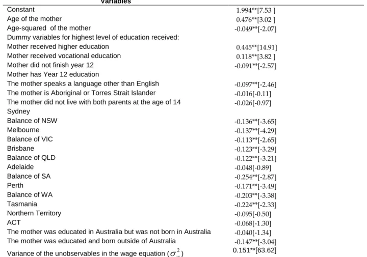
Table 3. Simulated maximum likelihood estimates –wage equation

Partnered mothers with at least one pre-school child, pooled estimates (2005-2007)

Variables

Constant 1.994**[7.53 ]

Age of the mother 0.476**[3.02 ] Age-squared of the mother -0.049**[-2.07] Dummy variables for highest level of education received:

Mother received higher education 0.445**[14.91] Mother received vocational education _{0.118**[3.82 ]} Mother did not finish year 12 -0.091**[-2.57] Mother has Year 12 education

The mother speaks a language other than English -0.097**[-2.46] The mother is Aboriginal or Torres Strait Islander -0.016[-0.11] The mother did not live with both parents at the age of 14 -0.026[-0.97] Sydney Balance of NSW -0.136**[-3.65] Melbourne -0.137**[-4.29] Balance of VIC _{-0.113**[-2.65]} Brisbane -0.123**[-3.29] Balance of QLD -0.122**[-3.21] Adelaide -0.048[-0.89] Balance of SA -0.254**[-2.87] Perth _{-0.171**[-3.49]} Balance of WA -0.203**[-3.38] Tasmania -0.224**[-2.33] Northern Territory -0.095[-0.50] ACT _{-0.068[-1.30]}

The mother was educated in Australia but was not born in Australia -0.040[-1.34] The mother was educated and born outside of Australia -0.147**[-3.04] Variance of the unobservables in the wage equation (σ_w2) 0.151**[63.62] t-values are in the brackets. * Significant at 10% level. ** Significant at 5% level.

The parameter estimates for the wage equation are presented in Table 3. The parameter estimates are in line with a standard Mincer equation for Australia

(see Breusch and Gray, 2004; Leigh, 2008; and Breunig et al., 2008 for a few examples). For example, higher education brings a wage premium of about 45 per cent for mothers of pre-school children, relative to their counterparts who only finished Year 12, and women who speak a language other than English earn less than those who do not.

4.2

Simulation results

Table 4 presents average elasticities of labour supply and child care demand with respect to mother's wage, other combined family income (partner's labour income and household non-labour income), gross child care price and net child care price for the full sample.

Labour supply and child care both have two components: the decision to participate and the decision of how much to participate. For the labour supply elasticities we report an employment (or participation) elasticity that addresses the question of whether or not people choose to work. The hours elasticity captures both changing hours for those who are already working and changing hours for those who decide to commence or cease working.

Similarly with child care, we provide an elasticity (use of formal care) which captures the decision to use child care or not. The hours elasticity captures both changing hours for those who are already using child care and changing hours for those who decide to commence or cease using child care.

Table 4. Elasticities: All partnered mothers with at least one pre-school child

With respect to Labour supply elasticity Child care demand elasticity Hours Employment Hours of formal care Use of formal care Gross child care price -0.106** (0.03) -0.070** (0.02) -0.294** (0.05) -0.166** (0.03) Net child care price -0.096** (0.03) -0.059** (0.01) -0.246** (0.04) -0.132** (0.02) Wage 0.427** (0.08) 0.274** (0.05) 0.281** (0.06) 0.176** (0.03) Household Income (other

than mother's earnings)

-0.092* (0.05) -0.048 (0.04) -0.036 (0.04) -0.036* (0.02)

4.2.1 Labour supply elasticities

First of all, it is worth noting that the estimates of wage and income elasticities of labour supply in Table 4 are in line with the literature (see for example, Breunig, et al., 2008 or Gong et al., 2010 which surveyed the estimates). For mothers with pre-school children, the average wage elasticities of hours worked and employment are 0.427 and 0.274 (significant at the 5 per cent level) and the income elasticities of hours worked and employment are -0.092 (significant at the 10 per cent level) and -0.048.

Secondly, the average labour supply elasticities of both gross and net child care price are statistically significant and negative. The average gross child care price elasticities of hours of work and employment for the mothers are -0.106 and -0.070, respectively, which means that for a one per cent increase in the gross child care price, on average, mothers’ hours of work would decrease by about 0.11 per cent and their employment rate would decrease by 0.07 per cent.

The net price elasticities of hours of work and employment of the mothers with pre-school children are -0.096 and -0.059, respectively. As expected, they are slightly smaller than the gross price elasticities due to the means-testing of CCB.

4.2.2 Relationship to previous results

These findings confirm those of Gong et al. (2010) that there is a negative and statistically significant labour supply response of partnered women to child care price. The estimates reported in Table 4 and those reported by Gong et al. (2010) are not statistically different from one another. However, Gong et al. (2010) report a higher point estimate of the gross price elasticity of employment of -0.29.

There are five reasons why the point estimates between the two studies might differ. Firstly, the two papers use a different estimation approach. In this paper, we directly specify the utility function and the household budget constraint. In Gong, et al. (2010), a linear approximation of the labour supply function that is consistent with the utility maximisation process is estimated.12

Fourthly, and the biggest difference between the two papers, is the way that child care prices are treated in the estimation of elasticities. One reason why one might expect smaller elasticities in this paper is that they are calculated with respect to a change in the child care price for pre-school children. In Gong et al. (2010), elasticities are reported with respect to a change in average child care price which means that all child care prices are changing, not just those for pre-school children. This difference is expected to lead to smaller estimates in this paper than in Gong et al. (2010). To confirm this point, we calculated gross child care price elasticities specific to pre-school children using the results from Gong et al. (2010). The employment elasticity of the child care price of pre-school Secondly, the two papers use different samples. This paper uses a sample of households which have at least one pre-school child whereas Gong, et al. (2010) use all households with children under the age of 13. Thirdly, the estimates reported in this paper are the ‘average elasticity’, which is the average of the elasticity across all observations. In Gong et al., the ‘elasticity of the average’ is reported, which is the elasticity calculated at the sample average. While it is clear that these three differences should result in different elasticity estimates, we have no a priori

beliefs about whether this should make elasticity estimates larger or smaller.

12 Gong et al. (2010) contains a lengthy discussion of the contrast between the `direct’ approach of this paper and the `indirect’ approach of that paper.

children is estimated to be about -0.15. Indeed, this is smaller than the estimate of -0.29 for the elasticity with respect to average (all) prices.

A fifth important difference between the two papers is that the model in this paper incorporates the quantity constraint on total child care hours equaling or exceeding mothers’ work hours while allowing formal child care hours to be less than the mothers' work hours.

4.2.3 Child care demand elasticities

As expected, child care demand is negatively impacted by its own price. From Table 4, the average net child care price elasticity of formal child care hours is -0.246; for a one per cent increase in the net child care price, child care hours decrease, on average, by about 0.25 per cent. The net elasticity of formal child care use with respect to its own price is -0.132, which means that a one per cent increase in the net child care price would lead to 0.132 per cent decrease in child care use.

The results in Table 4 show that both child care demand and labour supply elasticities with respect to wage are positive and they are both negative with respect to child care price. The two cross-price elasticities have the same sign as the own price elasticities (wage elasticity of labour supply and child care price elasticity of child care) which implies that labour supply and child care are complements.

As mentioned above, the assumption that child care of school-aged children mirrors that of pre-school children is quite strong. Estimation results and elasticities for an alternative specification, in which child care for school-aged children is assumed to be fixed and does not enter the utility function, are presented in Tables A.1.1 through A.1.4 of the Appendix. The simulated

elasticities are quite similar to the original specification. We conclude that this restriction does not matter for the substantive results.

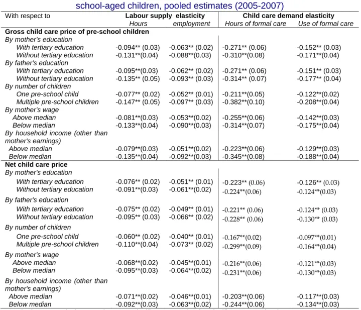
4.2.4 Elasticities of subsamples

The response of both labour supply and child care demanded might differ for households with different characteristics. For families where mothers’ participation in the labour market is more valuable (where the mother has higher wages) or for families which are more able to afford child care, we might see smaller responses to price changes. To better understand these effects, we split the samples in numerous ways related to mother's wage (by education and directly by mother's wage), household income (father's education and household income other than the mother's earnings) and number of children. We present