What Drives Default and Prepayment
on Subprime Auto Loans?
1
Erik Heitfield
Division of Research and Statistics
Federal Reserve Board
Washington, DC 20551 USA
202-452-2613
[email protected]
Tarun Sabarwal
Department of Economics
University of Texas at Austin
Austin, TX 78712 USA
512-475-8522
[email protected]
April 30, 2003
1We thank Robert Anderson, James Barth, Ron Borzekowski, Glenn Canner, Brad Case, Diana Hancock, Kumar Kanthan, Andreas Lenhert, and Greg Udell for valuable comments, and Irina Barakova and Mary DiCarlantonio for outstanding research assistance. The opinions expressed here are our own, and do not reflect those of the Federal Reserve Board or its staff.
Abstract
This paper uses novel data on the performance of loan pools underlying asset backed securities to estimate a competing risks model of default and prepayment on subprime automobile loans. We find that prepayment rates increase rapidly with loan age but are not affected by prevailing market interest rates. Default rates are much more sensitive to aggregate shocks than are prepayment rates. Increases in unemployment precede increases in default rates, suggesting that defaults on subprime automobile loans are driven largely by shocks to household liquidity. There are significant differences in the default and prepayment rates faced by different subprime lenders. Those lenders that charge the highest interest rates experience the highest default rates, but also experience somewhat lower prepayment rates. We conjecture that there is substantial heterogeneity among subprime borrowers, and that different lenders target different segments of the subprime market. Because of their higher default rates, loans that carry the highest interest rates do not appear to yield the highest expected returns.
1
Introduction
While lending to all types of households increased substantially during the 1990s, lending to households with limited financial resources and/or short or impaired credit histories – so-called subprime borrowers – has drawn particular attention from policy makers and bank regulators. Anecdotal evidence that subprime lenders have encouraged borrow-ers to refinance loans on unfavorable terms or have embedded obscure but expensive covenants in loan contracts have led to accusations that subprime lenders engage in “predatory” lending practices. The Home Ownership and Equity Protection Act, as well as legislation adopted by some state and municipal governments, has sought to redress these concerns by imposing additional reporting requirements and limiting spe-cific pricing policies and covenants on high-cost residential mortgages (Elliehausen and Staten 2002).
Even when loans are priced fairly, subprime borrowers, who by and large have lower and more volatile income and fewer assets than prime borrowers, may have particular difficulty making regular debt payments during times of economic stress. Bank regulators tasked with ensuring the safety and soundness of the US banking system have focused on the potential costs to banks and thrifts of large numbers of subprime loan defaults. In January 2001, after several federally insured financial institutions experienced severe losses on subprime loan portfolios, the Federal Reserve, the Office of the Comptroller of the Currency, the Federal Deposit Insurance Corporation, and the Office of Thrift Supervision jointly issued guidelines requiring stricter supervision of banks and thrifts engaged in subprime lending.
The need for greater regulation of subprime lenders is obviously closely linked to the question of whether the interest rates and fees charged on subprime loans are sufficient to adequately compensate financial institutions for the risks of lending to less credit-worthy borrowers. Yet although some lenders have developed proprietary models to underwrite subprime loans, very little academic research has examined the risks associated with subprime lending. In a unique study, Malmquist, Phillips-Patrick and Rossi (1997) use balance sheet data to examine the performance of savings and loan institutions that do substantial mortgage lending in low-income neighborhoods. They find that these S&Ls have higher costs including credit losses, but comparable profit rates, to S&Ls that do not lend in low-income neighborhoods. Balance sheet data do not permit a direct analysis of the causes of credit losses on S&L mortgage portfolios. A great deal of empirical research including recent work by Deng, Quigley and Van Order (2000),
Pavlov (2001), and Calhoun and Deng (2002) has used loan-level data to investigate the economic drivers of default and prepayment risks on residential mortgages, but none has explicitly examined the risks associated with subprime lending.
This paper seeks to broaden our understanding of subprime credit markets by exam-ining the sources of default and prepayment risks on subprime automobile loans. In many ways, automobile loans are similar to fixed rate residential mortgages. Both are held by households and are collateralized by tangible assets. Both are repaid using fixed-coupon amortization schedules, and both contain embedded default and prepayment options. Thus, one can expect insights into the behavior of borrowers and lenders in subprime automobile loan markets to shed light on the relationship between loan pricing and loan risk on subprime mortgages. An important advantage of studying automobile loans is that available data permit one to compare loan pricing and credit risk across a number of different lenders.
An improved understanding of the risks inherent in subprime automobile lending is also of value independent of what it tells us about other types of subprime lending, because automobile loans represent a significant portion of consumer debt. At the end of 1998, the last year for which figures are available, debt outstanding on all automobile loans was $447 billion, and accounted for 61 percent of non-revolving, non-mortgage consumer debt and 34 percent of all non-mortgage consumer debt. Although definitive data on the size of the growing subprime automobile loan market are not available, at the end of 2001, principal outstanding on loans in pools securitized by companies specializing in subprime automobile lending stood at $30 billion.
The primary impediment to empirical research on automobile lending is lack of data. Indeed, we are not aware of any publicly available disaggregated data on the performance of individual subprime automobile loans. However, as the loan backed securities market has developed, new data on the performance on pools of automobile loans have become available. Since the mid-1990s a number of finance companies have employed asset-backed securities to fund a large share of their automobile lending. Moody’s produces regular reports that combine information from SEC filings on securitization deals with information obtained directly from ABS issuers. Using these data, we have constructed a sample of 3,595 month-pool observations tracking the performance of 124 pools of automobile loans issued by 13 finance companies specializing in subprime lending.
The Moody’s data do not track individual loans, but rather provide pool-level ac-counting information that can be used to infer the total numbers of loans that default
and prepay during each month that a pool is active. Because of the aggregated nature of these data, standard loan-level competing risks models commonly used to investigate mortgage termination risks cannot be estimated directly. However, we show that if one assumes that all loans within a pool share the same hazard function, then a competing risks model can be estimated from pool-level data. This modeling approach enables us to investigate the effects of loan seasoning, aggregate shocks, and differences across loan issuers on subprime automobile loan default and prepayment rates.
We find that prepayment rates are high and increase rapidly with loan age, but are not affected by market interest rates. Subprime borrowers do not appear to refinance their loans in response to relatively small declines in prevailing interest rates. Instead they appear more likely to prepay their loans out of earned income, by refinancing to lower rate prime loans as their credit histories improve, or by selling their cars.
The hazard function for loan defaults is relatively flat. Unlike residential mortgage default hazard functions, it does not decline significantly toward the end of a loan’s life, perhaps because automobiles do not hold their values as well as real estate. Increases in unemployment rates precede increases in default rates, indicating that default rates on subprime automobile loans are particularly sensitive to shocks to household liquidity.
Our analysis reveals significant differences in the default and prepayment rates faced by different subprime lenders. Those issuers that charge the highest interest rates expe-rience the highest default rates, but also expeexpe-rience somewhat lower prepayment rates. This suggests that there is substantial heterogeneity among subprime borrowers, and that different issuers target different segments of the subprime market. Loans that carry the highest interest rates do not appear pay the highest returns net of default losses.
The paper proceeds as follows. Section 2 describes Moody’s loan-backed securities reports and explains how we extract aggregate pool performance information from the accounting data they provide. Section 3 presents a simple competing risks model of default and prepayment and shows how it can be estimated from aggregated pool-level data. An analysis of the effects of loan seasoning, aggregate shocks, and loan issuers on default and prepayment rates is presented in Section 4. Section 5 examines the relationship between loan interest rates and default and prepayment rates. Section 6 draws conclusions and discusses opportunities for future research.
2
Data
There exists no widely-accepted definition of a subprime borrower. In a March 3, 1999 guidance letter to bank supervisors, the major US bank regulators (the Office of the Comptroller of the Currency, the Federal Deposit Insurance Corporation, the Federal Reserve Board, and the Office of Thrift Supervision) define subprime lending as “ex-tending credit to borrowers who exhibit characteristics indicating a significantly higher risk of default than traditional bank lending customers.” In a January 31, 2001 guidance letter the regulators go further by proposing the following working definition of subprime borrowers:
Generally, subprime borrowers will display a range of credit risk character-istics that may include one or more of the following:
• Two or more 30-day delinquencies in the last 12 months, or one or more 60-day delinquencies in the past 24 months;
• Judgment, foreclosure, repossession, or charge-off in the prior 24 months;
• Bankruptcy in the last 5 years;
• Relatively high default probability as evidenced by, for example, a credit bureau risk score (FICO) of 660 or below (depending on prod-uct/collateral), or other bureau or proprietary scores with an equivalent default probability likelihood; and/or
• Debt service-to-income ratio of 50% or greater, or otherwise limited ability to cover family living expenses after deducting total monthly debt-service requirements from monthly income.
However, the guidance letter emphasizes that this definition is “illustrative rather than exhaustive.” Asset based loans with relatively poor collateral may also be classified as subprime. For example, some mortgage lenders view very high loan-to-value residential mortgages as subprime, and some automobile finance companies treat used car loans as subprime.
This study makes use of data on loans issued by automobile finance companies that Moody’s has identified as specializing in subprime lending. To establish this classifi-cation Moody’s relies on the representations of the companies themselves, as well as information on the characteristics of those companies’ typical borrowers. The finance companies identified by Moody’s are not the only providers of subprime automobile loans to consumers. Banks, thrifts, and finance companies that principally target prime
borrowers have also become involved in subprime lending in recent years. Lending from these institutions is not represented in our data.
Finance companies originate subprime automobile loans using a network of franchises and car dealers. They may fund this lending with traditional debt or equity, but in the 1990s many of these companies also began to issue asset-backed securities. In a typical automobile securitization, an originator pools several thousand automobile loans and sells these to a special-purpose entity such as a trust. The special-purpose entity, in turn, issues securities backed by a beneficial interest in the receivables from the loans in the pool. Typically, the originator continues to service the loans for a fee. Depending on credit enhancements, asset quality, servicer strength, and other variables, these securities are assigned a credit rating and can be traded in capital markets.
It is possible that the automobile loans that underly asset-backed securities are not representative of all loans made by finance companies. For example, some lenders may choose to “cherry pick” by securitizing only their relatively less desirable loans. We believe this potential source of selection bias is of limited practical importance because several of the largest finance companies represented in our sample have adopted explicit policies of securitizing all or nearly all of the loans they originate. Unfortunately, data comparing the characteristics of on- and off-balance sheet automobile loan portfolios are not publicly available.
Each issuer of publicly-traded automobile loan-backed securities submits periodic reports to the SEC documenting the performance of the underlying collateral pool. Using these data and other sources, Moody’s publishes New Issue Reports describing each collateral pool and Pool Performance Reports that track the performance of pools over time. Among the variables included in a typical New Issue Report are the initial weighted average interest rate (termed weighted average coupon, or WAC), the weighted average maturity, and the age of loans in a pool, as well as the initial number of loans and asset balance for the pool. Variables available on a monthly frequency from Pool Performance Reports include the principal balance on loans outstanding, delinquency rates, dollars charged-off, and dollars prepaid for active pools.
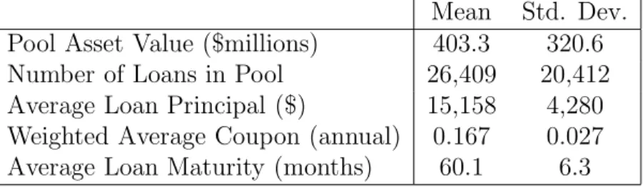
We have compiled sufficient data from Moody’s New Issue and Pool Performance reports to construct a sample of 3,595 pool-month observations on 124 loan pools from 13 different issuers. A total of 3.3 million automobile loans were held in these pools. Table 1 reports summary statistics for our sample of loan pools. Figure 1 provides information on pool issue dates, pool sizes, and WACs. Although some of the pools in
our sample were issued during 1994, 1995, and 1996, performance data for most pools are only available after 1996.
The fundamental unit of analysis for examining default and prepayment risk is the individual loan. The aggregate competing risks model described in Section 3 requires information on the number of loans that default and prepay in each month in the life of a pool. Because these data are not directly reported by Moody’s, we must infer them from available accounting data. To accomplish this, we first calculate the average remaining balance for active loans in a pool by using information on the pool’s average loan size, weighted average coupon, and maturity in a standard amortization formula. We then estimate the number of prepaid loans by dividing the reported dollars of principal prepaid in a month by the estimated average remaining loan principal balance for that month.
Estimating the number of loans that default in a month requires that we make an as-sumption about the relationship between charge-offs and loan defaults. We assume that when a loan defaults, sixty percent of its remaining principal is charged off. The number of loans that default is estimated by dividing the reported dollars charged off in a month by the estimated principal balance scaled to reflect the charge-off assumption. The sixty percent charge-off rule represents what we take to be a reasonable approximation of standard practice based on discussions with industry participants. Unfortunately, the detailed accounting data needed to either validate or generalize this simple rule are not publicly available. To the extent that our sixty percent charge-off assumption is too high (respectively, too low) we will under (over) predict default probabilities. Nonetheless, our conclusions about the economic drivers of default and prepayment risk should be robust to reasonable departures from this assumption.1
3
The Competing Risks Model
Several recent studies including Deng et al. (2000), Pavlov (2001), Ambrose and Sanders (2001), and Calhoun and Deng (2002) have used a competing risks framework to model loan default and prepayment. Unlike these studies, we observe information on the ag-gregate performance of loan pools rather than on individual loans. In this section, we
1The high charge-off rate is largely a result of the the costs associated with repossessing and selling
used cars. A large and reportedly better managed company in our sample reports charge-off rates on repossessed cars on the order of fifty percent. Industry analysts have suggested larger numbers for other finance companies. As a robustness check, we have estimated our model using a number of different fixed charge-off assumptions. Though higher charge-off assumptions result in lower overall predicted default rates, the qualitative features of our model are unaffected.
show how a standard competing risks framework can be modified to model aggregate pool performance data. Our approach makes use of the discrete outcome interpretation of duration models described by Allison (1982) in a general setting and by Shumway (2001) in an application to credit risk modeling.
Consider a pool of N0 loans with a maturity of T months. At the end of month t, an active loan must arrive in one of three states; it must remain active, default, or be paid off. A loan that has neither defaulted nor been paid off by the end of montht−1 is said to have survived to month t. If a loan does not survive it drops out of the pool, so the number and composition of loans remaining in a loan pool changes from month to month.
Let Sit be an indicator variable that is equal to one if loan i has survived to month t and zero otherwise. Letyit be a discrete variable that is equal to one if loan idefaults in month t, two if it is prepaid in month t, and zero otherwise. We assume that, conditional on observable time-varying, pool-level variables, transitions to default or prepayment are independent across loans and follow a non-homogeneous Markov process. The hazard rate for default (respectively, prepayment) is the probability that a loan defaults (prepays) in month t given that it has survived to the end of month t−1. We model these hazard rates using a simple multinomial logit specification of the form
hjt ≡P [yit=j | Si,t−1 = 1] = exp(µ
j t)
1 + exp(µ1t) + exp(µ2t) (1) where j = 1 corresponds to default and j = 2 corresponds to prepayment. µ1t and µ2t are index functions of model parameters and exogenous variables that vary across pools and time, but not across obligors within a pool. Using a result from Lancaster (1990, page 12), it can be shown that the probability that loan isurvives to the end of month t is Ht≡P [Sit= 1] = t Y s=1 1 + exp(µ1s) + exp(µ2s) !−1 . (2)
In the language of duration models, Ht is called a survival function. If the time paths of µ1t andµ2t are known, then (1) and (2) can be used to calculate cumulative and monthly
survival, default, and prepayment probabilities.
We cannot observe yit because we do not have loan-specific performance data. How-ever, by using the methods described in Section 2, we can infer the number of loans that
default and prepay during each month in the life of a loan pool. LetNtbe the number of loans in a pool that are active at the end of montht, and letn1t and n2t be the numbers of loans that default and prepay in month t. By definitionNt =Nt−1−n1t−n2t. LetNt
be the vector of observed active loan counts from months one tot, and letn1t and n2t be the corresponding vectors for default and prepayment counts.
Since all loans in a pool share the same hazard rates, the number of loans that survive, default, and prepay in montht conditional on the number of loans active at the end of month t−1 have the multinomial distribution
PNt, n1t, n2t | Nt−1= Nt−1! Nt!n1t!n2t! 1−h1t −h2tNt ht1n1t h2tn2t . (3) Furthermore, the Markov assumption implies that
PNt, n1t, n2t | Nt−1 = PNt, n1t, n2t | Nt−1,
so we can write the likelihood function for the history of observed defaults and prepay-ments over the life of the pool as
L NT,n1T,n2T | N0=
T
Y
t=1
PNt, n1t, n2t | Nt−1. (4) Given data on defaults and prepayments for a number of pools, the parameters of the index functions µ1t and µ2t can be estimated by maximum likelihood.
The hazard rate index functions depend on a pool’s age, calendar time, and the pool’s issuer. Using a specification similar to that of Gross and Souleles (2002), we assume
µjt = 4 X s=1 (t)sβsj + Q X q=1 dqτqj+ K X k=2 Ikηkj, (5)
where dq is an indicator variable identifying calendar quarter q, and Ik is an indicator variable identifying pool issuer k. Greek letters denote model parameters. Note that because we include a full set of quarter dummies, one issuer dummy must be dropped.
The probabilities of default and prepayment for older loans are likely to be different from those associated with more recent loans because borrowers’ financial circumstances tend to evolve over time. For example, refinancing opportunities may increase with loan age as a borrower demonstrates an ability to manage credit effectively. Changes in the
relationship between the value of collateral backing a loan and the value of the loan itself may also affect a borrower’s incentive to prepay or refinance. The fourth-order polynomials of t in µ1 and µ2 permit a broad range of patterns of smooth changes in default and prepayment hazard rates.
Permitting pool default probabilities to depend on calendar time allows us to cap-ture the effects of systematic shocks that affect loans in all pools. Rather than explicitly including a list of macroeconomic variables in the index function, we use vectors of quar-ter fixed effects. This allows us to remain agnostic about the dequar-terminants of aggregate shocks that are likely to affect default and prepayment rates, and ensures that omitted macroeconomic variables will not induce biases in our estimates of seasoning and issuer effects.
Including pool issuer fixed effects in the specifications of µ1 and µ2 allows for the possibility that loans originated by some issuers have higher default or prepayment hazard rates than others. Such differences could be important if, for example, different issuers specialize in lending to different segments of the subprime market.
4
Results
Our empirical specification isolates the effects of loan age (seasoning), calendar time, and loan issuer on default and prepayment probabilities. In this section we examine each of these effects in turn.
4.1
Loan Seasoning
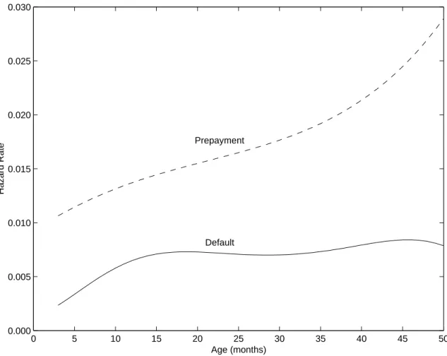
Figure 2 plots estimated hazard functions for loan default and prepayment holding time and issuer effects constant at their sample means. Parameter estimates for the fourth-order polynomials in loan age that generate these curves are reported in Table 2.
The default hazard function rises for the first year and levels off or increases only slightly thereafter. The tendency for default hazard rates to increase during the early months in the life of a loan has been well documented in previous research on residential and commercial mortgages. It seems reasonable to expect that loan officers and auto-mated credit scoring models are more effective in identifying and screening out obligors who are likely to default over the near term than over the medium or long term. As finan-cial conditions change over time, the ability of some obligors to make regular payments will naturally deteriorate, causing default hazards to rise.
Prior research on residential mortgages has found that after reaching a peak, default hazard rates tend to fall (Deng et al. 2000, Calhoun and Deng 2002). A common explanation for this empirical regularity focuses on the relationship between the value of a mortgage and the value of its underlying collateral. As a mortgage ages, the value of the loan declines while the value of the real estate collateralizing the loan tends to grow. Defaults rates decline as falling loan-to-value ratios increase the relative cost of default to borrowers. We find little evidence of declining hazard rates late in the life of subprime automobile loans. Unlike real estate, the value of an automobile tends to decline over time. Thus loan-to-value ratios for automobile loans may not fall very rapidly, and may well increase over some portion of the life of a loan.
As can be seen in Figure 2, prepayment hazard rates are much higher than default hazard rates and rise quickly with loan age. There are several possible explanations for the increasing duration dependence of loan prepayments. As a loan ages and its principal is paid down, it becomes easier for an obligor to prepay the remaining principal out of earned income. Moreover, an obligor’s ability to refinance the loan at more favorable terms may increase as he or she builds a stronger credit history. Finally, many obligors undoubtedly choose to prepay when selling their cars. An obligor is presumably less likely to sell a car in the early months of a loan shortly after the car was purchased.
4.2
Aggregate Shocks
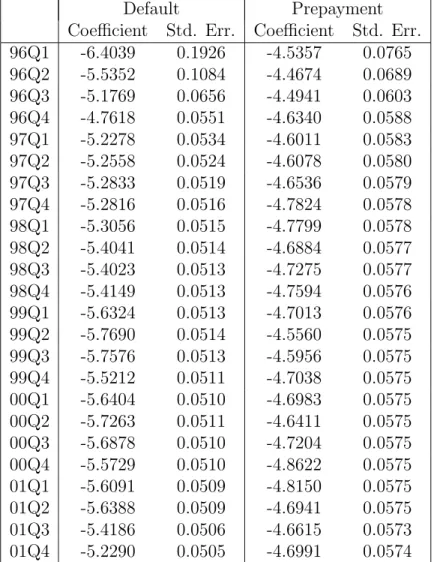
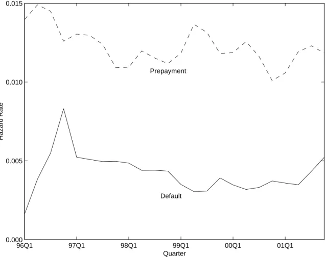
Default and prepayment probabilities for all subprime automobile loans can be expected to rise and fall as macroeconomic conditions change. Our competing risks model captures these aggregate effects by allowing for quarter-specific shocks that affect the default and prepayment probabilities of all currently active loans. Figure 3 shows predicted default and prepayment hazard rates for a six-month-old loan holding issuer effects constant at the sample average. Estimated parameter values are reported in Table 3.
Because they affect all obligors, aggregate shocks to prepayment and default prob-abilities pose risks that are more difficult for lenders to manage than shocks that are idiosyncratic to individual obligors. Idiosyncratic risk can be easily diversified away, while systematic risk must be hedged. To evaluate the relative importance of system-atic shocks in determining default and prepayment rates, we calculated the interquartile range of each time series of quarter fixed effects and divided by the median fixed effect. This volatility measure is similar to the more common volatility statistic calculated by dividing a time series’ standard deviation by its mean, but is more robust to
measure-ment errors in the estimated fixed effects. Our volatility measure is 0.065 for the default fixed effects and 0.026 for the prepayment fixed effects, indicating that aggregate shocks play a much larger role in determining loan defaults than loan prepayments.
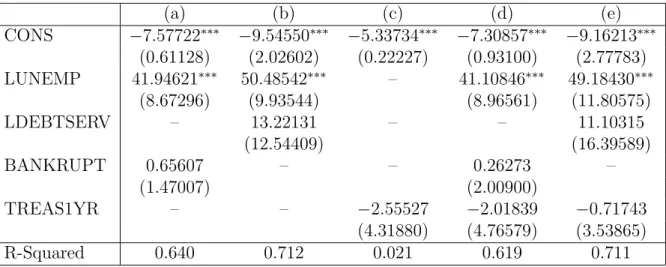
To examine the effects of macroeconomic conditions on default and prepayment prob-abilities, the estimated quarter fixed effects were regressed on an array of aggregate vari-ables. Explanatory variables are described in Table 4, and results are reported in Tables 5 and 6.2 The one-quarter lagged civilian unemployment rate, the one-quarter lagged aggregate household debt-service burden, and the number of personal bankruptcy cases filed were included to account for aggregate changes in households’ ability to repay or prepay their loans.3 One-year treasury rates were included to examine the possibility that falling interest rates might make refinancing more desirable.4
Regressions (a) and (b) in Table 5 most accurately reflect ourex antebeliefs about the factors that drive aggregate changes in default rates. Increases in the unemployment rate unambiguously lead aggregate changes in default rates. These effects are both statistically and economically significant. The point elasticity of the default hazard rate with respect to the unemployment rate evaluated at the sample mean is 1.94 in regression (a) and 2.24 in regression (b). Both the household debt-service burden and total bankruptcies were trending upward throughout the time period of our data, so we cannot meaningfully distinguish between the effects of these two variables. Neither is statistically significant, though both have the expected sign. We find no evidence that current treasury rates affect default hazards.
A large body of empirical research has found a strong negative correlation between prevailing interest rates and residential mortgage prepayment rates. As can be seen from columns (c), (d), and (e) in Table 6, we find little evidence that auto loan prepayment rates increase as prevailing interest rates fall. This may be because there are fewer direct refinancing opportunities available to subprime auto loan borrowers, or because
2In each regression, a feasible generalized least squares procedure was used to correct for
het-eroscedasticity arising from differences in the precision with which each of the quarter fixed effects were estimated.
3Except in the case of bankruptcy, loans are not generally written off until they are at least 120
days past due. Thus we expect the unemployment rate and the household debt-service burden to lead defaults by at least a quarter. Other specifications were run in which real variables were either not lagged or were lagged two or more quarters. These regressions produced similar though weaker results. Because the data span only 24 quarters, a more detailed analysis of the timing of real variables and default and prepayment rates was not possible.
4Three, five, and ten-year treasury rates were also examined, but they had no greater explanatory
the benefits associated with auto loan refinancing are much smaller than those associated with mortgage refinancing.
Other macroeconomic variables may affect prepayment rates if, for example, finan-cially stressed households find it more difficult to prepay their high rate loans. The household debt-service burden and the number of personal bankruptcy cases are not statistically significant, but do have the expected sign. Unexpectedly, the unemploy-ment rate appears to be positively correlated with prepayunemploy-ments. The elasticity of the prepayment hazard rate with respect to the unemployment rate ranges from 0.46 un-der regression (b) to 0.52 unun-der regression (d). These figures are much lower than the corresponding default hazard elasticities.
4.3
Differences Among Subprime Lenders
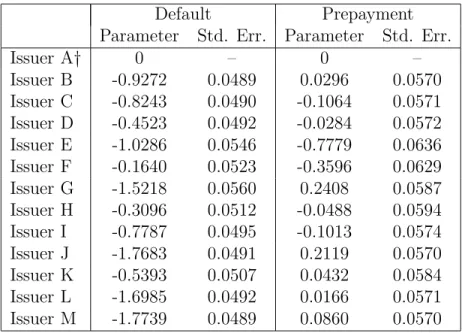
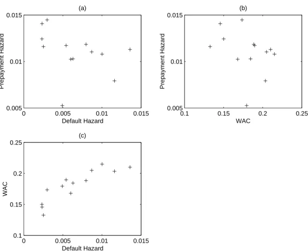
Issuer-specific fixed effects in our competing risks model allow for the possibility that different subprime lenders experience systematically different default and prepayment rates. These fixed effects are reported in Table 7. Similar information is displayed in Panel (a) of Figure 4, which plots the default and prepayment hazard rates for a six-month-old loan for each issuer holding time effects constant. The correlation between default and prepayment issuer fixed effects is -0.33, indicating that those lenders that experience higher default rates also tend to experience lower prepayment rates.
Differences in prepayment and default rates across issuers can arise whether or not there is significant heterogeneity among subprime borrowers. If all subprime borrowers were homogeneous, then differences in observed default and prepayment rates could arise from differences in underwriting or collections policies across issuers. If, as seems more likely, there is substantial heterogeneity among subprime borrowers, then differences across issuers could also arise if different issuers choose to lend to different types of borrowers.
The negative relationship between default and prepayment rates that we observe is consistent with the view that (1) borrowers who are most able to prepay their loans are least likely to default, and (2) different subprime lenders target different segments of the subprime market. As will be shown in the next section, further support for this conjecture can be found by examining the relationship between loan interest rates and default and prepayment rates.
5
The Pricing of Subprime Automobile Loans
The weighted average coupon (WAC) for a pool measures the annualized average interest rate charged on loans in that pool at origination. This is an effective measure of the interest rate charged on active loans throughout the life of a pool because nearly all subprime automobile loans carry fixed rates. A regression of pool weighted average coupon on a vector of dummy variables identifying each of the 13 issuers in our sample reveals that issuer identity alone explains 96.5 percent of the cross-pool variation in interest rates. When quarter dummies are added the explanatory power of the regression rises only slightly to 97.7 percent, and we cannot reject the hypothesis that the quarter fixed effects are jointly equal to zero. Thus, our data provide strong evidence that the interest rate charged on a subprime automobile loan is much more closely linked to the finance company making the loan than to prevailing economic conditions at the time the loan was made. In light of the strong link between issuer and weighted average coupon, the analysis that follows treats the issuer as the unit of analysis for examining the relationship between interest rates charged and default and prepayment probabilities.
There are several reasons to believe that loan interest rates are related to prepayment and default probabilities. From a lender’s perspective, the most profitable subprime customers are those that neither default nor prepay. To the extent that either form of premature loan termination can be predicted by lenders, differences in risks should be priced into the interest rate charged to borrowers. Causality can also work in the opposite direction. As Stiglitz and Weiss (1981) point out, higher risk borrowers have fewer available financing opportunities so those borrowers who are likely to accept higher interest rate loans can be expected to have higher default rates than those who accept lower rate loans. Finally, interest rates may directly affect borrower behavior. Borrowers faced with the high monthly payments associated with high interest rate loans may have more difficulty making regular loan payments. Furthermore, borrowers with the means have a stronger incentive to rapidly prepay higher rate loans. Given the limitations of available data, we cannot distinguish among these different causal links between interest rates and default and prepayment risks. We can, however, assess the extent to which the interest rates charged by different lenders are correlated with these risks.
Panels (b) and (c) of Figure 4 plot the predicted one-month default and prepayment hazard rates for a six-month-old loan for each issuer against the average WAC of that issuer’s loans. Panel (c) shows a strong positive relationship between default probabili-ties and interest rates, while Panel (b) shows a somewhat weaker negative relationship
between prepayment probabilities and interest rates. The correlation between an issuer’s average WAC and its default fixed effect is 0.92. The correlation between an issuer’s average WAC and its prepayment fixed effect is -0.26. The negative correlation between interest rates and prepayment rates is somewhat surprising, since borrowers paying the highest interest rates have the strongest incentives to prepay their loans. However, it is consistent with the market segmentation hypothesis outlined in Section 4.3. If dif-ferent subprime lenders focus on difdif-ferent segments of the subprime market, then one would expect those lenders that specialize in serving the riskiest customers to charge the highest interest rates. Furthermore, if high risk borrowers are the least able to prepay their loans, then we should observe a negative correlation between prepayment rates and interest rates.
Given the observed positive correlation between interest rates and default rates, it is natural to ask whether the high interest rates charged on subprime loans are sufficient to compensate lenders for the high default probabilities associated with these loans. We examine this question by comparing the interest rates charged by each issuer with the internal rate of return (IRR) of that issuer’s loans.
The IRR is the annualized discount rate required to set the net present value of an expected stream of cash flows equal to the value of the original investment. In the context of the model presented here, the internal rate of return is given by IRR= (1 +δ)12−1 where δ solves 1 = T X t=1 (h1tλ+h2t)Pt+ (1−h1t −h2t)M (1 +δ)t Ht,
Pt is the share of original principal outstanding in month t, M is the monthly loan
payment as a proportion of original principal, andλ is the recovery rate on a defaulted loan.5 Given the weighted average coupon and the weighted average maturity of a loan pool, Pt and M are calculated using a standard amortization formula. It is important to emphasize that these IRR figures do not directly reflect the costs associated with originating or servicing loans, nor do they reflect the opportunity cost of capital. Taken by themselves, they cannot tell us which lenders made the most profitable loans. They can, however, provide an indication of whether loan interest rates fully reflect cross-issuer differences in default rates.
5As discussed in Section 2, we assumeλ= 0.4. Changing this assumption does not substantively
affect estimated IRRs. Higher recovery assumptions imply higher predicted default rates. These two effects tend to cancel out one another in the IRR calculation.
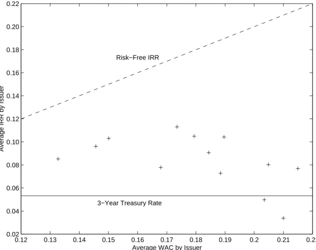
The dashed line in Figure 5 shows the theoretical relationship between WAC and IRR in the absence of loan defaults and prepayments. Default losses reduce a loan’s internal rate of return, so expected IRRs will always lie below this line. The solid line shows the average three-year Treasury rate during the sample period. The crosses plot the average internal rate of return for loans from each issuer (holding time effects constant) against the average interest rate charged by that issuer.
The average estimated IRR taken across all loans in the sample is 9.6 percent, which is much lower than the 16.0 percent average interest rate charged on these loans but is significantly higher than the 5.3 percent yield paid on a comparable-maturity Treasury bond during the sample period. According to the Federal Reserve’s G-19 statistical release, the average interest rate charged at origination on 48-month new car loans issued by commercial banks between 1996 and 2001 was 8.8 percent. Since this figure does not net out default losses, it is an upper bound on the expected yield for prime loans. Thus, it would appear that subprime loans provided, on average, a higher expected yield than prime rate automobile loans during the sample period.
The expected IRR is an estimate of a loan’s yield after adjusting for expected losses due to default and prepayment. This return measure does not make adjustments for the greater variability in losses on loans made to higher risk borrowers. Therefore, the presence of a risk-premium for more volatile income streams would imply a positive relationship between loan interest rates and IRR. In contrast, the correlation between issuer average WAC and issuer average IRR is -0.52, indicating that higher loan interest rates tend to be more than offset by higher default rates. This suggests that risk-based pricing alone cannot explain cross-issuer differences in interest rates.
6
Conclusion
In many ways subprime automobile loans are similar to fixed-rate residential mortgages. Both are secured by assets, both are repaid on fixed-coupon amortization schedules, and both carry fixed interest rates. Nonetheless, our analysis reveals some important differences between the economic factors that affect defaults and prepayments on these two types of loans.
Research on residential mortgages consistently finds a strong negative relationship between prevailing market interest rates and prepayment rates, suggesting that mortgage holders strategically exercise prepayment options. We find no evidence that market
interest rates are related to prepayment rates on subprime automobile loans, but we do find that prepayment hazard rates increase rapidly with loan age. Thus, subprime borrowers do not appear to refinance their automobile loans when prevailing interest rates fall, but do exhibit a strong tendency to prepay loans out of earned income, by shifting to lower prime-rate loans as their credit histories improve, or by selling their cars.
Loan-to-value ratios (LTVs) play an important role in explaining default rates on residential mortgages. As a mortgage ages and its principal is paid down, its LTV falls and default becomes less likely. We find little evidence of falling default hazard rates late in the lives of subprime automobile loans. Unlike real estate, the value of an automobile tends to decline over time, so a loan’s LTV may not fall very rapidly, and may well increase during some portion of the loan’s life. We find a strong positive relationship between default rates and unemployment rates, suggesting that defaults on subprime automobile loans are particularly sensitive to shocks to household liquidity.
Disaggregated data would permit a more thorough analysis of the effects of loan seasoning on default and prepayment rates. Although our empirical specification allows for differences in borrowers across pools, it does not explicitly model within-pool obligor heterogeneity. Because of this, it is possible that the hazard functions we estimate reflect not only the effects of a loan’s age, but also the effects of changes in the composition of active loans in a pool. For example, the default rate for a pool may increase with its age because the lowest-risk obligors in that pool tend to prepay their loan early and drop out. Han and Hausman (1990), Sueyoshi (1992), and Deng et al. (2000) have proposed methods for modeling unobserved heterogeneity in a competing risks framework, but these approaches are not directly applicable to aggregated data. In the absence of detailed loan-specific information, strong assumptions about the shape of default and prepayment hazard functions and the distribution of unobserved heterogeneity within pools would be needed to separate the effects of loan seasoning from changes in pool composition.
An important advantage of the Moody’s pool performance data used in this study is that they permit comparisons of loan pricing and credit risk across subprime lenders. Our analysis reveals a strong positive correlation between the interest rates an issuer charges and the average default rates of its borrowers, and a somewhat weaker negative correlation between those interest rates and prepayment rates. These empirical regu-larities suggest that those borrowers who are most likely to default are least likely to
prepay, and that different issuers focus on different segments of the subprime market. Loans carrying the highest interest rates do not appear to yield the highest expected returns, suggesting that risk-based pricing alone cannot explain observed cross-issuer differences in interest rates. Without information on the credit-worthiness of individual borrowers it is impossible to determine whether differences in interest rates are a cause or an effect of differences in default and prepayment rates. Disaggregated data that include information on the performance of individual loans as well as the characteristics of individual borrowers would go a long way toward improving our understanding of the link between interest rates and automobile loan default and prepayment rates.
References
Allison, Paul D., “Discrete-time Methods for the Analysis of Event Histories,” in Samuel Leinhardt, ed., Sociological Methodology: 1982, Jossey-Bass, 1982.
Ambrose, Brent and Anthony B. Sanders, “Commercial Mortgage-backed Securi-ties: Prepayment and Default,” August 2001. Working Paper.
Calhoun, Charles A. and Yongheng Deng, “A Dynamic Analysis of Fixed- and Adjustable-Rate Mortgage Termination,” Journal of Real Estate Finance and Eco-nomics, January 2002, 24 (1), 9–33.
Deng, Yongheng, John M. Quigley, and Robert Van Order, “Mortgage Ter-minations, Heterogeniety and the Exercise of Mortgage Options,” Econometrica, March 2000,68 (2), 273–307.
Elliehausen, Gregory and Michael Staten, “Regulation of Subprime Lending Prod-ucts: An Analysis of North Carolina’s Preditory Lending Law,” September 2002. Working Paper.
Gross, David B. and Nicholas S. Souleles, “An Empirical Analysis of Personal Bankruptcy and Delinquency,” Review of Financial Studies, Spring 2002, 15 (1), 319–347.
Han, Aaron and Jerry A. Hausman, “Flexible Parametric Estimation of Duration and Competing Risk Models,” Journal of Applied Econometrics, 1990, 5, 1–28.
Lancaster, Tony, The Econometric Analysis of Transition Data Econometric Society Monographs, Cambridge University Press, 1990.
Malmquist, David, Fred Phillips-Patrick, and Clifford Rossi, “The Economics of Low-Income Mortgage Lending,” Journal of Financial Services Research, 1997,
11, 169–188.
OCC, FRB, FDIC, and OTS, “Interagency Guidance on Subprime Lending,” March 1999. FDIC Press Release PR8a-99.
, , , and , “Expanded Guidance for Subprime Lending Programs,”
Pavlov, Andrey D., “Competing Risks of Mortgage Termination: Who Refinances, Who Moves, and Who Defaults?,” Journal of Real Estate Finance and Economics, September 2001, 23(2), 185–211.
Shumway, Tyler, “Forecasting Bankruptcy More Accurately: A Simple Hazard Model,” Journal of Business, 2001,74 (1), 101–124.
Stiglitz, Joseph E. and Andrew Weiss, “Credit Rationing in Markets with Imperfect Information,” American Economic Review, June 1981, 71 (3), 393–410.
Sueyoshi, Glenn T., “Semiparametric proportional hazards estimation of competing risks models with time-varying covariates,”Journal of Econometrics, 1992, 51, 25– 58.
Mean Std. Dev. Pool Asset Value ($millions) 403.3 320.6 Number of Loans in Pool 26,409 20,412 Average Loan Principal ($) 15,158 4,280 Weighted Average Coupon (annual) 0.167 0.027 Average Loan Maturity (months) 60.1 6.3
Table 1: Sample statistics for subprime auto loan pools.
Default Prepayment Parameter Std. Err. Parameter Std. Err. AGE 2.930E-1 3.814E-2 5.052E-2 1.072E-3 AGE2 -1.619E-2 2.895E-4 -1.869E-3 1.160E-4 AGE3 3.729E-4 8.592E-6 3.626E-5 4.811E-6 AGE4 -3.010E-6 8.650E-8 -1.961E-7 4.840E-8 Table 2: Loan seasoning curve parameter estimates (βs).
Default Prepayment Coefficient Std. Err. Coefficient Std. Err. 96Q1 -6.4039 0.1926 -4.5357 0.0765 96Q2 -5.5352 0.1084 -4.4674 0.0689 96Q3 -5.1769 0.0656 -4.4941 0.0603 96Q4 -4.7618 0.0551 -4.6340 0.0588 97Q1 -5.2278 0.0534 -4.6011 0.0583 97Q2 -5.2558 0.0524 -4.6078 0.0580 97Q3 -5.2833 0.0519 -4.6536 0.0579 97Q4 -5.2816 0.0516 -4.7824 0.0578 98Q1 -5.3056 0.0515 -4.7799 0.0578 98Q2 -5.4041 0.0514 -4.6884 0.0577 98Q3 -5.4023 0.0513 -4.7275 0.0577 98Q4 -5.4149 0.0513 -4.7594 0.0576 99Q1 -5.6324 0.0513 -4.7013 0.0576 99Q2 -5.7690 0.0514 -4.5560 0.0575 99Q3 -5.7576 0.0513 -4.5956 0.0575 99Q4 -5.5212 0.0511 -4.7038 0.0575 00Q1 -5.6404 0.0510 -4.6983 0.0575 00Q2 -5.7263 0.0511 -4.6411 0.0575 00Q3 -5.6878 0.0510 -4.7204 0.0575 00Q4 -5.5729 0.0510 -4.8622 0.0575 01Q1 -5.6091 0.0509 -4.8150 0.0575 01Q2 -5.6388 0.0509 -4.6941 0.0575 01Q3 -5.4186 0.0506 -4.6615 0.0573 01Q4 -5.2290 0.0505 -4.6991 0.0574
Table 3: Estimated quarter fixed effects (τs).
Variable Description Mean Std. Dev.
LUNEMP Lagged unemployment rate 0.04640 0.00528 LDEBTSERV Lagged household debt service burden 0.13566 0.00357 BANKRUPT Personal bankruptcy cases (millions) 0.32597 0.03072 TREAS1YR 1-year treasury rate 0.05126 0.01020 Table 4: Macroeconomic variables used to explain aggregate shocks to default and pre-payment probabilities.
(a) (b) (c) (d) (e) CONS −7.57722∗∗∗ −9.54550∗∗∗ −5.33734∗∗∗ −7.30857∗∗∗ −9.16213∗∗∗ (0.61128) (2.02602) (0.22227) (0.93100) (2.77783) LUNEMP 41.94621∗∗∗ 50.48542∗∗∗ – 41.10846∗∗∗ 49.18430∗∗∗ (8.67296) (9.93544) (8.96561) (11.80575) LDEBTSERV – 13.22131 – – 11.10315 (12.54409) (16.39589) BANKRUPT 0.65607 – – 0.26273 – (1.47007) (2.00900) TREAS1YR – – −2.55527 −2.01839 −0.71743 (4.31880) (4.76579) (3.53865) R-Squared 0.640 0.712 0.021 0.619 0.711
Standard errors appear in parentheses.
*, **, and *** denote 90%, 95%, and 99% significance respectively.
Table 5: Feasible generalized least squares regressions of default hazard quarter fixed effects on macroeconomic variables.
(a) (b) (c) (d) (e) CONS −4.91618∗∗∗ −4.49211∗∗∗ −4.74635∗∗∗ −4.94250∗∗∗ −4.97000∗∗∗ (0.25587) (1.13757) (0.09005) (0.32756) (1.39643) LUNEMP 10.44773∗∗∗ 9.85022∗∗ – 10.51240∗∗∗ 11.12985∗∗ (2.94360) (4.72619) (2.98671) (5.13293) LDEBTSERV – −4.66778 – – −1.98857 (7.01918) (8.37205) BANKRUPT −0.73018 – – −0.69414 – (0.47166) (0.54987) TREAS1YR – – 1.24237 0.22789 1.07874 (1.73858) (1.75606) (1.84786) R-Squared 0.574 0.468 0.044 0.574 0.486
Standard errors appear in parentheses.
*, **, and *** denote 90%, 95%, and 99% significance respectively.
Table 6: Feasible generalized least squares regressions of prepayment hazard quarter fixed effects on macroeconomic variables.
Default Prepayment Parameter Std. Err. Parameter Std. Err.
Issuer A† 0 – 0 – Issuer B -0.9272 0.0489 0.0296 0.0570 Issuer C -0.8243 0.0490 -0.1064 0.0571 Issuer D -0.4523 0.0492 -0.0284 0.0572 Issuer E -1.0286 0.0546 -0.7779 0.0636 Issuer F -0.1640 0.0523 -0.3596 0.0629 Issuer G -1.5218 0.0560 0.2408 0.0587 Issuer H -0.3096 0.0512 -0.0488 0.0594 Issuer I -0.7787 0.0495 -0.1013 0.0574 Issuer J -1.7683 0.0491 0.2119 0.0570 Issuer K -0.5393 0.0507 0.0432 0.0584 Issuer L -1.6985 0.0492 0.0166 0.0571 Issuer M -1.7739 0.0489 0.0860 0.0570 † Issuer A omitted.
Weighted Average Cost
Pool Issue Date
94-Dec 95-Dec 96-Dec 97-Dec 98-Dec 99-Dec 00-Dec 01-Dec
0.100 0.150 0.200 0.250
Figure 1: Loan pool issue dates and weighted average coupons. The area of each circle is proportional to the number of loans in the pool at the issue date.
0 5 10 15 20 25 30 35 40 45 50 0.000 0.005 0.010 0.015 0.020 0.025 0.030 Age (months) Hazard Rate Default Prepayment
Figure 2: Default and prepayment hazard functions, holding time and issuer effects constant.
96Q1 97Q1 98Q1 99Q1 00Q1 01Q1 0.000 0.005 0.010 0.015 Quarter Hazard Rate Prepayment Default
Figure 3: Quarterly one-month default and prepayment hazard rates for a six-month-old loan, holding issuer effects constant.
0 0.005 0.01 0.015 0.005 0.01 0.015 Default Hazard Prepayment Hazard (a) 0.1 0.15 0.2 0.25 0.005 0.01 0.015 WAC Prepayment Hazard (b) 0 0.005 0.01 0.015 0.1 0.15 0.2 0.25 Default Hazard WAC (c)
Figure 4: Default hazard rates, prepayment hazard rates, and Weighted Average Coupon by issuer. Default and prepayment hazard rates are for six-month-old loans holding time effects constant.
0.12 0.13 0.14 0.15 0.16 0.17 0.18 0.19 0.2 0.21 0.22 0.02 0.04 0.06 0.08 0.10 0.12 0.14 0.16 0.18 0.20 0.22
Average WAC by Issuer
Average IRR by Issuer
3−Year Treasury Rate Risk−Free IRR