Measuring Monotonicity in Multiclass Classification

(1)

UNIVERSITY OF TARTU

Institute of Computer Science

Computer Science Curriculum

Joonas Kriisk

Measuring monotonicity in multiclass

classification

Bachelor’s Thesis (9 ECTS)

Supervisor: Mari-Liis Allikivi, MSc

Supervisor: Meelis Kull, PhD

(2)

Measuring monotonicity in multiclass classification

Abstract: Machine learning is a field in computer science where the main purpose is to create a method which can make predictions about data. Multiclass classification is a task in machine learning where the solution is to classify an object into one of at least three classes based on real-life observations. After training the model, it is usually necessary to somehow evaluate the accuracy of the model. This is usually done by splitting data into two sets - training and test set - and testing the trained model against the test set. Models output scores, which show the confidence of the prediction. In the process of decision making, it is very helpful if these scores could be interpreted as class probabilities. Calibration is used to convert these scores to probabilities. Having prediction errors can have negative consequences in certain applications, so it is necessary for models to be well calibrated. Most popular and widely used binary calibration method is isotonic regression, it fits a free-form line to scores, but there is a constraint - the line must be non-decreasing everywhere. For multiclass cases, a reduction to binary task is mostly done to use isotonic regression but this once again means that scores need to be monotonous. Consequently it is logical to check if this also holds true in multiclass problems as this can help in developing multiclass calibration methods.

This Bachelor’s thesis focuses on measuring the monotonicity by creating multiple machine learning models on different datasets. But to measure monotonicity, we first had to come up with ways on how to measure it - for this thesis we proposed two different methods. First method ranks all probabilities base on a single class probabilities resulting in a one-vs-rest comparison. Second method takes top50%probabilities of two classes (to reduce the noise made by third class), ranks them and this results in a one-vs-one comparison. Main result of the experiment is that71,4%of dataset-model pairs seem to be monotonic while the monotonicity of non-monotonic pairs seems to be highly affected by having low accuracy on all models on these datasets.

An empirical study was conducted on 21 datasets where on each set 7 models were trained. Two different measurement methods were used to calculate monotonicity and based on results these two methods have similar outcomes and seem to be affected by the accuracy of the model. Monotonicity in multiclass datasets has not been researched before and this research provides insight on if multiclass sets are monotonic or not.

Many models nowadays are used widely in marketing, banking and medicine and having calibrated models is a necessity. Knowing that multiclass datasets are monotonic now gives the opportunity to devise a more efficient calibration method on multiclass problems.

Keywords: machine learning, multiclass classification, monotonicity, empirical study

(3)

Monotoonsuse mõõtmine mitmeklassi klassifitseerimisprobleemidel

Lühikokkuvõte:Masinõpe on arvutiteaduste valdkond, mille põhieesmärgiks on luua meetodid, mis suudavad teha ennustusi andmete põhjal. Mitmeklassi klassifitseerimis-ülesande puhul on lahenduseks klassifitseerida objekt ühte vähemalt kolmest võimalikust klassist, kasutades selleks vaadelduid andmeid. Peale mudeli treenimist, on vaja kuidagi ka mudeli täpsust hinnata. Üldiselt tehakse andmestik kaheks - treening- ja testandmeteks - ja mudeli täpsust testitakse testandmete peal. Mudelid väljastavad skoore, mis

näita-vad ennustuse enesekindlust. Otsustuste tegemise protsessis on eriti kasulik, kui need skoorid on tõlgendatavad klasside tõenäosustena. Kalibreerimist kasutatakse skooride tõenäosuseks konverteerimisel. Vead ennustamistel võivad olla negatiivsete tagajärgeda, kui neid kasutataks teatud teatud valdkondades ja viisidel, seega on tähtis, et mudelid oleksid hästi kalibreeritud. Kõige laialt levinum binaarne kalibreerimismeetod on isotoo-niline regressioon, see sobitab vaba joone skooridele, aga sellel on üks kitsendus - joon peab olema mittelangev. Mitmeklassi klassifitseerimisel üldiselt vähendatakse probleem binaarsele tasemele, et sellel saaks jätkuvalt rakendada isotoonilist regressiooni, aga see eeldab, et skoorid oleksid monotoonsed. Seega on ainult loogiline uurida, kas mitme-klassi mitme-klassifitseerimisel monotoonsus peab paika, sest see aitaks luua uusi mitmemitme-klassi kalibreerimismeetodeid.

Antud bakalaureuse lõputöö keskendub monotoonsuse mõõtmisele luues mitmeid masinõppe mudeleid erinevate andmestike peal. Mõõtmiseks teostamiseks tuli ka välja mõelda viis, kuidas seda teha - tööraames pakkusime välja kaks meetodit. Esimene meetod järjestab kõik tõenäosused ühe klassi raames, luues üks-vs-ülejäänud võrdluse. Teine meetod võtab kahe klassi parimad 50%tõenäosustest (et vähendada kolmanda klassi mõju andmepunktidel) ja järjestab need ning luues seega üks-vs-üks võrdluse. Töö peamine tulemus on, et71,4%andmestik-mudel paaridest on monotoonsed ning mittemonotoonsete paaride monotoonsus sõltub suuresti sellest, et andmestikel, kus mudeleid treeniti, oli kõikide mudelite täpsus madal.

Viidi läbi empiiriline uuring 21 andmestiku peal, kus igal andmestikul treeniti 7 masinõppe mudelit. Monotoonsuse mõõtmiseks kasutati kaht eri mõõtmismeetodit ja tulemuste põhjal võib öelda, et mõlemal mõõtmismeetodil on sarnased resultaadid ning monotoonsust mõjutab mudeli täpsus. Monotoonsust mitmeklassi andmestike peal ei ole varasemalt uuritud ja vastav lõputöö annab ülevaate, kas sellised andmestikud on monotoonsed või ei.

Masinõpe on igapäevaelus laialt kasutuses - reklaamid, pangandus, meditsiin ja seetõttu on vajalik, et mudelid oleksid hästi kalibreeritud. Teades, et mitmeklassi andmes-tikud on monotoonsed, siis see annab võimaluse luua efektiivsema kalibeerimismeetodi vastavatel andmestikel.

(4)

(5)

3.2.1 Logistic regression . . . 13 3.2.2 Naive Bayes . . . 14 3.2.3 Decision Tree . . . 14 3.2.4 Random Forest . . . 14 3.2.5 Bagging . . . 14 3.2.6 AdaBoost . . . 15 3.2.7 Multilayer Perceptron . . . 15 3.3 Structure of experiment . . . 15 4 Results 16 4.1 Predicted probabilities . . . 16 4.2 Calculated monotonicities . . . 19 5 Summary 23 References 24 II. Licence . . . 25

(6)

1 Introduction

The general goal of machine learning is to understand the structure of data and fit them into machine learning models which can be understood and used by humans. In this thesis we are using supervised learning methods in which models are provided with input and output data that is previously labeled. The reason for this kind of action is that the algorithm will learn by comparing its actual outputs with given outputs to find errors and further modify the model appropriately.

Multiclass classification is a classification task with more than two classes - for an example a classification model is tasked with classifying a set of images of pets which may be dogs, cats, or rabbits. Multiclass classification makes the assumption that each sample is assigned to one and only one class: a pet can either be a dog or a cat but not both at the same time, meaning they are mutually exclusive. When performing classification we often want not only to predict the class label, but also obtain the probability of the label. This probability will give us some kind of confidence on the prediction. Some models can give you poor estimates of the class probabilities and some even do not support probability prediction. To get a better estimation of probabilities the model needs to be calibrated.

Having a calibrated classifier means classifier scores can be directly interpreted as class membership probabilities. A well calibrated binary classifier should classify the instances such that to which samples it gave a predicted probability value close to0.8, approximately80%actually belong to the positive class as well.

For binary cases, most used calibration method is isotonic regression (monotonic regression). Monotonic means that the function does not have to exclusively increase, but it most not decrease. Isotonic regression fits a free-form line to instances, but there is a constraint: the fitted line has to be non-decreasing everywhere. This is why we say binary calibration methods assume that the classifier outputs monotonous scores. During binary calibration, higher classifier scores will be mapped to higher probabilities, because it is assumed that base classifier outputs higher scores for the positive class. This is why it is logical to build calibration functions which maintain this property.

For multiclass cases, most of the time a reduction to binary task is used and this means that for isotonic regression, it needs to be monotonous. Therefore it is necessary to check if this also holds true in multiclass datasets as this could help in developing multiclass calibration methods. The main focus of this thesis is to do an empirical study on multiple different real datasets and analyze them and to find out if multiclass problems have a similar monotonous property compared to binary cases.

In the following chapters, it will be explained what methods will be used to measure monotonicity, how to calculate it, an empirical study ranging over multiple datasets will be conducted, what models will be used and an analysis of the results gathered from the study.

(7)

2 Measuring monotonicity

Before machine learning model will be given a set of data to train on, the original set will be split into two - training data and test data - this just means that the data will be split in e.g. 75/25ratio. Both training data and test data contain inputs and outputs. Model will be trained on the training data, where it learns the rules and finds patterns to predict label values on unlabeled data. In evaluation phase, model will be tested against the test data - model is given the input of test data, but not the output, and it will try to predict the output data. This prediction can be seen as a vector of probabilities for each class e.g. (0.2,0.5,0.3): probability of label being class 1 is0.2, for class 2 it is0.5and for class 3

it is0.3. In addition, the sum of probabilities is always 1. There will be as many vectors of predicted probabilities as there are instances in the test data. These probabilities will be plotted as dots onto a standard 2-simplex graph (see Figure 1), where each of the corners correspond to a class. The color of the dot will be determined by its true label. Colors of the corners indicate the true class of an instance - red: class 1, green: class 2, blue: class 3. This means that the bigger the probability of class 1 is, the closer the the dot will be to the red corner, because each corner represents a probability of 1.

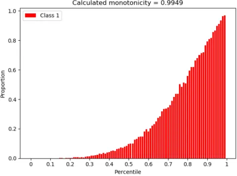
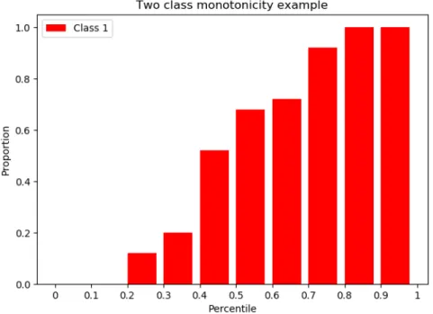
For a binary case, the monotonicity is found in the following way: all of predicted probabilities will be ranked on the basis of one class, ranked probabilities will be split into multiple bins where in each bin the proportion of true class 1 elements will be found. Here is an example of how a two class classification monotonicity looks like (Figure 1). Probabilities were split into 10 bins and in each bin the corresponding proportion of true class 1 elements was calculated. And since it is a binary case, this means that if one class is monotonic, then the other class must also be monotonic.

(8)

Figure 1. Example of a monotonic two-class classification

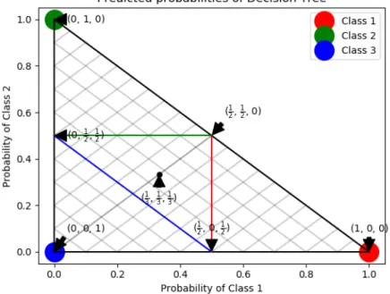
For multiclass case, if one class appears to be monotonic, you cannot say if the other remaining two classes are monotonic. Because of this reason, we had to come up with some kind of method on how to measure monotonicity for each class and secondly, how to calculate it based on measurement results. To measure monotonicity in multiclass cases, we decided on two different methods. In the first method, all of the data points would be projected onto a line which runs straight down the middle for a given class -projected onto the red line in case of class 1 (as can be seen on Figure 2).

(9)

Figure 2. Example of 2-simplex with lines for ranking [3]

For an example, a predicted probability of class 1 - meaning (0.2,0.5,0.3)would become (0.2,0.8), where probability of class 1 stays the same, but the probabilities of other two classes will be added. This results in a one-vs-rest comparison and now enables a binary case comparison for the probabilities. The line will be separated into 100 bins and each bin would contain an equal amount of instances. In each of the bins the proportion of the corresponding class (in our case class 1) will be calculated. It is fair to assume that the closer to 0 percent we are observing, the smaller the proportion will be, and as we move upwards towards 1, the proportion should increase. This will be done for each class and a corresponding metric will be calculated - this will be introduced later on in this chapter - and if monotonicity for each of the classes is above the threshold, we can say that data is monotonic for this method.

To illustrate, let’s say we have these ten predicted probabilities: (0.3,0.3,0.4), (0.25,0.7,0.05),(0.8,0.1,0.1),(0.6,0.1,0.3),(0.25,0.25,0.5),(0.55,0.25,0.2),(0.1,0.3,0.6), (0.7,0.15,0.15),(0.15,0.3,0.55),(0.45,0.2,0.35). For each probability vector, the class with the highest probability is also the true class meaning for (0.3,0.3,0.4), class 3 is the true class. If we use method 1 to calculated the monotonicity of class 1, then after projecting, the probabilities would become(0.3,0.7),(0.25,0.75),(0.8,0.2), (0.6,0.4),(0.25,0.75),(0.55,0.45),(0.1,0.9),(0.7,0.3),(0.15,0.85),(0.45,0.55). Af-ter ranking them based on class 1 probabilities, the vectors would be in this order:

(10)

(0.1,0.9), (0.15,0.85), (0.25,0.75), (0.25,0.75), (0.3,0.7), (0.45,0.55), (0.55,0.45), (0.6,0.4), (0.7,0.3), (0.8,0.2). Splitting these into 3 bins would result in such bins -bin 1: [(0.1,0.9),(0.15,0.85),(0.25,0.75),(0.25,0.75)], bin 2: [(0.3,0.7),(0.45,0.55), (0.55,0.45)], bin 3: [(0.6,0.4),(0.7,0.3),(0.8,0.2)]. In each of the bins, the number of true class 1 labels will be counted and divided by the total number of elements in the bin to get the proportion of class 1 elements. In bin 1, there are 0 true class 1 labels, so the proportion is0. In bin 2, there are two true class 1 labels, so the proportion is 2₃. In bin 3, all the elements are true class 1 labels, meaning the proportion is1. So the proportions are0, 2₃ and1in this order.

For method two, the 2-simplex will be divided into a top and bottom half (Figure 3). The elements of the top half will be ignored, because in method 2 we are measuring the monotonicity of the two opposite classes - if we look at the red line which corresponds to class 1, then the bottom half means opposite of the class corner and therefore left of the red line and the monotonicity of class 2 and class 3 will be measured. In addition, all true instances of class 1 will be ignored completely. Furthermore, the bottom half elements will be normalized - if we take class 1 as an example again, a vector of(0.2,0.5,0.3) would become(0,0.625,0.375). This means that all elements will end up on the side of simplex and once again, 100 bins will be created just like in method 1, but this time the proportion of class 2 will be calculated (proportion for class 3 will be the exact opposite).

(11)

To illustrate method 2, let’s take the same ten predicted probabilities from last example: (0.3,0.3,0.4),(0.25,0.7,0.05),(0.8,0.1,0.1),(0.6,0.1,0.3),(0.25,0.25,0.5), (0.55,0.25,0.2),(0.1,0.3,0.6),(0.7,0.15,0.15),(0.15,0.3,0.55),(0.45,0.2,0.35). Let’s say we want to measure monotonicity of class 2 compared to class 3, this means that we will only look at probability vectors where the sum of class 2 and class 3 probabil-ity is higher than0.5and we will ignore all true class 1 labels. After all this we are left with these vectors: (0.3,0.3,0.4),(0.25,0.7,0.05),(0.25,0.25,0.5),(0.1,0.3,0.6), (0.15,0.3,0.55). We will ignore the probability of class 1 and normalize the probabilities

of class 2 and class 3 and after this we will have these vectors:(0.43,0.57),(0.93,0.07), (0.33,0.67),(0.33,0.67),(0.35,0.65). These will be sorted by class 2 probability, result-ing in: (0.33,0.67),(0.33,0.67),(0.35,0.65),(0.43,0.57),(0.93,0.07). Splitting these into 3 bins again, we will have - bin 1: [(0.33,0.67),(0.33,0.67)], bin 2: [(0.35,0.65), (0.43,0.57)], bin 3: [(0.93,0.07)]. Bin 1 and bin 2 contain0true class 2 labels, bin 3

contains1true class 2 label - resulting proportions are0,0and1.

In order to measure and not just to observe, monotonicity should be calculable. If there are 100 bins, then there are 100₂∗99 = 4950 pairs between bins. We say a pair is in correct order if the bin which is closer to 0 percentile has lesser proportion of corresponding class compared to the other bin. The percent of correct pairs of all pairs is the calculated monotonicity.

If we want to calculate the monotonicity for the two previous examples, then there are no pairs that are in wrong order, meaning that for both methods the calculated monotonicity is1.

We calculate monotonicity for all three classes with both methods and if the mean of both methods is over0.9, we can conclude that the dataset is monotonous. Why the threshold was picked at 0.9, will be explained in chapter 4. Below is an example of AdaBoost class 1 bins using method 1:

(12)

(13)

3 Empirical study

3.1 Datasets

We used 21 datasets to conduct the monotonicity study upon them. All of the datasets contain atleast 10000 instances, as this helps us avoid over-fitting, reduces the impact of outliers and calibration methods need additional amount of instances to be able to create a calibration function.

9 datasets had 1 million instances, 3 datasets had less than 15000 and rest were between 100,000 and 700,000. 10 datasets had 3 classes and the rest had between 5-7. Most of the datasets had around 40 features, while 1 had 9 features and 2 datasets had over 100 - 129 and 127 respectively. 14 datasets had mostly numeric features, meaning 7 had mostly symbolic features. Interestingly most datasets had only 1-3 of the lesser feature - if a dataset had 36 numeric features, then it only had 1 symbolic feature. 2 sets had only numeric or symbolic features.

3.2 Machine learning models

We used the most popular classification algorithms to obtain the predicted probabilities necessary for measuring monotonicity. We also included ensemble methods such as bagging, boosting and random forest classification. An ensemble method is created by aggregating multiple outputs made by a diverse set of predictors to obtain better results. In addition, one artificial neural network model was used - the Multilayer Perceptron. Multiple different models were used to lessen the risk of monotonicity relying solely on the machine learning model and to obviously get different results. Support Vector Machines (SVM), a very popular model, was omitted due to scalability issues regarding the model - the time complexity is betweenO(n2₎_and_O₍_n3₎_{where n is the amount of}

training instances [4]. Since most of the used datasets have over 100,000 instances, it is not feasible to train SVM models. Most of models are used as they "out-of-the-box" - meaning none of the hyper-parameters are tuned - as improving the accuracy of the model is not the goal and neither necessity for this work. Multiple models are used to get different probabilities for the same dataset - this gives us insight to see if worse or better models have any difference in monotonicity.

3.2.1 Logistic regression

Multinomial logistic regression is a classification method that utilizes logistic regression to solve multiclass problems. Logistic regression is an algorithm involving a linear discriminant and unlike linear regression, logistic regression does not try to predict actual value of a numeric variable, but instead outputs a probability that the value belongs to a certain class. The multinomial logistic model assumes that each feature

(14)

(independent variable) has a single value for each case and that the actual class cannot be perfectly predicted for any case. Logistic regression uses a linear predictor function f(k, i) = β0,k + β1,kx1,i + β2,kx2,i +· · ·+ βM,kxM,i to predict the probability that

observationihas outcomek. [1] 3.2.2 Naive Bayes

Naive Bayes is a classification method on Bayes’ Theorem. It’s called naive because of the assumption of independence among features. This means that a Naive Bayes classifier assumes that the presence of a feature in a class is unrelated to the presence of any other feature. [5]

3.2.3 Decision Tree

Decision tree models use a decision tree as a predictive model to go make observations about an instance and conclude it’s target class. The tree begins with a root (where we still have all our observations) then comes a series of branches whose intersections are called nodes and ends are called leaves, each corresponding to one of the classes to predict. The depth of the tree is refers to the maximum number of nodes before reaching a leaf. In decision tree model, the leaves represent class labels and branches represent conjunctions of features that lead to those labels.

3.2.4 Random Forest

Random forest is an ensemble learning method for classification that operates by con-structing a multitude of decision trees at training time and outputting the class that is the mode of the classes of the individual trees. Random forest builds multiple decision trees and merges them together to get a more accurate and stable prediction. In addition, random forest corrects for decision trees’ habit of overfitting to their training set. [2] 3.2.5 Bagging

Bootstrap aggregating, also called bagging, is a machine learning ensemble designed to improve the stability and accuracy of machine learning algorithms used in classification and regression. The bootstrap method refers to generating additional data for training from original dataset using combinations with repetitions to produce multiple sets. This decreases variance and helps to avoid overfitting. This allows the model to get a better understanding of the various biases, variances and features.

(15)

3.2.6 AdaBoost

AdaBoost, short for Adaptive Boosting, is a one of many boosting methods. Boosting is a general method for improving the accuracy of any given learning algorithm. The boosting algorithm calls the base learning algorithm multiple times, each time with a different distribution or weighting over the training set. Due to weighting, some samples might be run more often than others. When boosting runs each model, it tracks which data samples are most successful and which are not - the ones with most misclassified outputs will be given heavier weights and are deemed to be more complex and require more iterations to train models properly.

3.2.7 Multilayer Perceptron

Multilayer perceptron is an artificial neural network model. It is composed of more than one perceptron, which is a single neuron model. They are composed of an input layer to receive the input, an output layer that makes a decision or prediction about the input, and in between those two, an arbitrary number of hidden layers that are the true computational engine of the model. The power of neural networks come from their ability to learn the representation in your training data and how to best relate it to the output variable that you want to predict.

3.3 Structure of experiment

The data was split into a training set and a test set with a0.75/0.25ratio and before training, feature scaling was applied to the data. Feature scaling is a method used to standardize the range of features of data, this is also known as data normalization. Since the range of values can vary widely, some machine learning algorithms do not work properly without such normalization.

On all of the datasets, 7 previously mentioned machine learning models were trained. All of the models were used as out-of-the-box with the exception of decision tree. Two different decision trees were trained, one without any limitations and one where the max depth of the tree was limited to 3. This was done to deliberately have a model which would have a lower accuracy compared to the rest of the models and to see how the monotonicity would be affected by this.

After training, the measuring of monotonicity was done as described in chapter 2. For each model and each class, predicted probabilities and the monotonicity were plotted as explained previously.

(16)

4 Results

We are using method 1 and method 2 to measure the monotonicity of each class in a dataset. Measuring is done on every model trained on the dataset and through this we can form a dataset-model pair. Before we explain the results, we expect to see that most pairs are monotonic and we believe that even multiclass datasets are monotonic.

(a) Example of high monotonicity, method 1 (b) Example of low monotonicity, method 2 Figure 5. Examples of monotonicities

(a) Method 1 compared to method 2 (b) Method 1 values compared to accuracy

Figure 6. Method 1 compared to method 2 and accuracy

4.1 Predicted probabilities

(17)

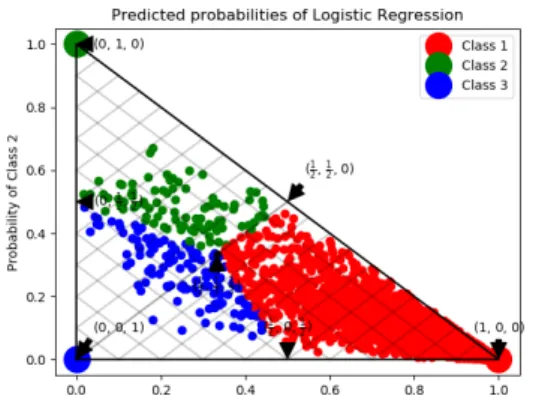
this simplex influences the monotonic relationship between dataset and classes. It should be noted that random 10,000 instances were only plotted as adding any more would have resulted in most points covering each other and much of the graph would have stayed the same. In addition, graphs which were plotted using a very high accuracy model were omitted from this showcase as most instances ended up in their respective class corners and most of the graph was empty. On Figure 7a, it can be seen that most dots have converged into the corners or sides 2-simples, meaning the calculated monotonicity and accuracy are going to be high. On Figure 7d, it can be seen that most dots have converged into the middle of graph, meaning the accuracy of the model is low, low accuracy also affects the monotonicity which in this case is also lower than0.85on both cases. On Figure 8a, it can be seen that class 2 and class 3 instances have converged to the side of graph, meaning that these instances according to model definitely do not belong to class 1. It is also a fair example of model having low accuracy, but still having high method 1 monotonicity. Figure 8b is a good example of how a good monotonicity looks like on a predicted probabilities graph.

(18)

(a) Accuracy: 0.9374, method 1: 0.9832, method 2:0.9773 (b) Accuracy: 0.9085, method 1: 0.9725, method 2:0.9533 (c) Accuracy: 0.6651, method 1: 0.8662, method 2:0.8507 (d) Accuracy: 0.5062, method 1: 0.8382, method 2:0.8494

(e) Accuracy: 0.5605, method 1: 0.9042, method 2:0.8347

(f) Accuracy: 0.8029, method 1: 0.9665, method 2:0.9504

(19)

4.2 Calculated monotonicities

Monotonicities were calculated for each class separately using method 1 and pair-wise for method 2. Average monotonicity for a dataset was calculated as mean of all class values per method. Although variance between calculated monotonicities wasn’t too high, it still resulted in very different graphs. Figures 8a and 8d are beautiful examples of monotonic class. Figures 8b and 8c are the outcomes of method 2, which means that "Class 1 vs Class 2" between class 1 and class 2 is monotonic relation. Figures 9a and 9b are examples of what a low monotonicity looks like, although accuracy of model on 9b is quite high, it still resulted in low monotonicity.

(a) Accuracy:0.9085

(b) Accuracy:0.7214, this is also an example of a model having low accuracy but still high monotonicity

(c) Accuracy:0.9085 (d) Accuracy: 0.8419

(20)

(a) Accuracy:0.8119

(b) Accuracy: 0.9277, this is an example of a model having high accuracy, but low mono-tonicity

Figure 9. Examples of low monotonicity

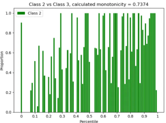
On 9 datasets, there was a single class which had a reasonably lower monotonicity compared to other classes. In 3 of these cases, more than 3 models had this problem, in other cases only 1 or 2 models had it, but in all cases it occurred with method 2 and only 2 times with both methods. It seems accuracy has a much higher effect on method 2 than it has on method 1. Below will be a few examples of such cases:

(a) Monotonicity:0.979 (b) Monotonicity:0.7374 (c) Monotonicity:0.9921

(21)

Figure 11. Method 2 monotonicities of Random Forest model, accuracy: 0.8064

Figure 12. Method 2 monotonicities of Bagging model, accuracy:0.7203

A dataset-model pair is counted as monotonic if the average calculated monotonicity for both methods was over0.9. Although pairs appeared to be certainly monotonic at around threshold of0.95, the threshold was set to0.9, because many pairs appeared to be monotonic, but often the calculated monotonicity would be around0.90−0.93for these cases and it was only logical to include these as well.

In total, there were 168 pairs and 120 of these were monotonic meaning that71,4% of all pairs were monotonic. 73 (61%) of these pairs had model accuracy over 0.9, meaning that39%of pairs had model accuracy less than that. In addition,12.75% of monotonic pairs had accuracy lower than0.8. The mean and median of accuracy of non-monotonic pairs were both0.62so it’s safe to assume that accuracy has a big impact on monotonicity. 14 (29%) of non-monotonic pairs actually had accuracy and calculated monotonicity based of method 1 higher than 0.8and 0.9and reaching up to 0.9 and 0.97respectively. This means that method 2 was less forgiving out of the two methods. Furthermore, most pairs that were non-monotonic, had lower monotonicity because the accuracy of all the models were quite low on some datasets.

While comparing the results of the two methods, they seemed rather equal; comparing the mean and median of all pairs -0.94vs0.93and0.97vs0.96. Based solely on accuracy, it seems that having accuracy of at least0.8results in having high monotonicity with both

(22)

methods as there were no outliers where a model would have an accuracy higher than 0.8but monotonicity lower than0.9. Observing Figure 6a, it can be noted that method 1 and method 2 seem to have a strong linear correlation with a few outliers. Method 1 compared to accuracy seems to indicate the same thing, but not quite to call it a strong linear correlation. Based on the results of the empirical study, we can infer that in our experiment the datasets indeed were monotonous, but the experiment was not big enough to be able to conclude that most multiclass datasets are monotonous as well.

(23)

5 Summary

This thesis gives a brief overview of multiclass classification and calibration and why having monotonic data is assumed for calibration. An experiment is then conducted to see if data is monotonic in multiclass cases as well. To test if data is monotonic, two methods are introduced on how to measure monotonicity and a way to calculate it based on the result of these two methods. 7 different machine learning models are trained on 21 datasets to have a wide variety of dataset-model pairs as inputs for measuring monotonicity.

From the results of the empirical study, we can deduce that both methods of measuring monotonicity give somewhat equal results as mean and median for both methods were 0.94vs0.93and 0.97vs0.96. In addition, it can be assumed that accuracy of a model plays a big role to measure if dataset-model pair is monotonic - there were no models where accuracy of the model was greater than 0.8, but monotonicty were lower than 0.9. Furthermore, we can conclude that according to these models and datasets, most multiclass datasets are definitely monotonic, because71,4%of all pairs were monotonic. Most pairs that were non-monotonic belonged to datasets, which in general had a comparatively low model accuracy across all models (0.6vs mean of0.9).

It is to be noted that datasets were chosen randomly and none of the hyper-parameters of the models were tuned. These two reasons can vary the result of the experiment, because accuracy of a model has a high impact on monotonicity and tuning of hyper-parameters can increase the accuracy. Moreover, there are many more models which can be used and which might have a different outcome

These results can now be taken into consideration when creating a new calibration method as calibration methods assume that data is monotonic.

The research on this topic can be continued. One could add more data, more models, fine-tune the existing models and even devise a new method on how to calculate mono-tonicity. It can be said that the data seems to be monotonic, but to give a final definitive answer a bigger scale study should be done.

(24)

References

[1] William H. Greene. In:Econometric Analysis. Boston: Pearson Education, 2012, pp. 803–806.ISBN: 978-0-273-75356-8.

[2] Robert Hastie Trevor; Tibshirani. In:The Elements of Statistical Learning (2nd ed.).

Springer, 2008.

[3] Jan Hendrik Metzen.Probability Calibration. Retrieved 14.05.2018 fromhttps: //jmetzen.github.io/2015-04-14/calibration.html. 2015. URL:https:// jmetzen.github.io/2015-04-14/calibration.html(visited on 05/14/2018). [4] Hans Simon and Nikolas List. “SVM-Optimization and Steepest-Descent Line

Search.” In:COLT 2009 - The 22nd Conference on Learning Theory. Jan. 2009. [5] K. Stuart A.; Ord. In:Kendall’s Advanced Theory of Statistics: Volume I—Distribution

(25)

I. Licence

Non-exclusive licence to reproduce thesis and make thesis public

I,Joonas Kriisk,

1. herewith grant the University of Tartu a free permit (non-exclusive licence) to: 1.1 reproduce, for the purpose of preservation and making available to the public,

including for addition to the DSpace digital archives until expiry of the term of validity of the copyright, and

1.2 make available to the public via the web environment of the University of Tartu, including via the DSpace digital archives until expiry of the term of validity of the copyright,

of my thesis

Measuring monotonicity in multiclass classification supervised by Mari-Liis Allikivi and Meelis Kull

2. I am aware of the fact that the author retains these rights.

3. I certify that granting the non-exclusive licence does not infringe the intellectual property rights or rights arising from the Personal Data Protection Act.