Area Biplots
J.C. Gower
∗P.J.F. Groenen
†M. van de Velden
‡November 1, 2007
Econometric Institute Report EI 2007-48
∗Statistics Department, The Open University, Milton Keynes, MK7GAA, United Kingdom
†Econometric Institute, Erasmus University Rotterdam, P.O. Box 1738, 3000 DR Rotterdam, The Netherlands
‡Econometric Institute, Erasmus University Rotterdam, P.O. Box 1738, 3000 DR Rotterdam, The Netherlands
Abstract
Classical multivariate analysis techniques such as principal components analysis and corre-spondence analysis use inner products to estimate data values. The results of these techniques may be visualized by representing the row and column points jointly in a biplot where the projection of a row point onto a column point vector followed by a multiplication by the length of the column point vector gives the inner-product that estimates the corresponding data element. In this paper, we propose a new visualization: after a 90◦rotation of the row
points, the areas spanned by a triangle of a row point, a column point and the origin estimate the data values. In contrast to the projection biplot, the areas spanned by different row and column points can be compared directly. Areas can only be produced for two dimensions at a time, but higher dimensional solutions can be represented by summing areas over subsequent pairs of dimensions. Here, the area biplot is developed for principal components analysis, correspondence analysis, and for interaction biplots but has general applicability.
Keywords: Biplot, Correspondence Analysis, Interaction, Principal Component Analysis, Visual-ization
1
Introduction
In many methods of multivariate analysis, one is faced with evaluating an inner product c0d.
Computationally there could hardly be anything more trivial but because of the strong visual component to some of these multivariate methods there is a need for a simple visual appreciation of inner products. The conventional visualization involves projectingcontodand multiplying the result by the length of the vectord. However, it is difficult to compare the estimates of the inner products that do not have the samecor d; the comparison is only straightforward when eitherc
or dis common to both inner products. This problem may be avoided by calibrating the vector
dwith the values of the inner product which may then be read off by projectingcontod; this is the basis of calibrated biplot methods. Calibrating the vectorscanddamounts to treating them like conventional coordinate axes. In this paper, we discuss a new alternative visualization, the
area biplot, that uses area to estimate the inner product. By definition areas are two-dimensional,
but we show that it is easy to combine more than one two-dimensional visualizations to visualize a higher dimensional solution.
The best known biplot is the principal components (PCA) biplot (Gabriel, 1971) where the relations between the samples and the variables are given by inner products. These relations are
often visualized by a two-dimensional display in which the samples are represented by points and the variables by vectors, although a reverse representation is also possible. Technically, it is not necessary to limit the biplot display to two dimensions, but it is the most convenient and most frequently used.
The remainder of this paper is organized as follows. In the next section, the biplot for PCA is defined explicitly. Section 3 introduces the area biplot for PCA. Then, in Sections 4 and 5, we show how our method can also be applied in correspondence analysis (CA) and biadditive models. Two examples of area biplots, are given in Section 6. We end with a discussion and some conclusions.
2
The PCA Biplot
For the moment, and without loss of generality, assume thatXis column centered, that is,10X= 00, where1denotes a vector of ones of the appropriate order and, similarly,0denotes a vector of
zeroes. Throughout the paper we shall use this notation. PCA can be expressed as minimizing
L(C,D) =kX−CD0k2= n X i=1 p X j=1 (xij−c0 idj)2, (1)
where C is ann×k matrix withk-dimensional coordinates for the n sample points and D is a p×k matrix with thepvariable vectors. Note that c0
i is row i of C andd0j is row j ofD. The dimensionality k is chosen by the researcher and is typically smaller than the rank of the data matrix. If a visualization of the data is required, kis often set to 2.
It is well known that (1) can be minimized by using the singular value decomposition (SVD) of
X, that is, X=UΣV0 with Σ a diagonal matrix with nonnegative singular values in decreasing
order, withUandVorthonormal matrices. LetU2andV2denote the first two columns ofUand VandΣ2the diagonal matrix with the two largest singular values. Then, a two-dimensional PCA
solution is obtained by choosingCpca=U2Σ2andDpca=V2. Note that, in this standardization,
the singular values are distributed over the row points. The estimation ofxij is done by evaluating the inner productc0
idj= (u0i2Σ2)vj2, whereui02is rowiofU2andvj02is rowjofV2. Furthermore,
by using this standardization, the distances between the sample points, that is the rows of Cpca approximate the inter-sample distances; the distances between the rows of X(e.g., Gower, 1966). For the estimation of the inner-products, the standardization is not important. For example, if we define C =qU2Σ12−α and D = q−1V2Σα2 the inner product matrixCD0 still approximates the
In the two-dimensional setting, the inner productc0
idj may be written as
c0
idj=kcik kdjkcos(θij) (2)
where kcikdenotes the Euclidean length of vectorci, that is,kcik= (c2i1+c2i2)1/2, andθij is the
angle between the vectorsci anddj. In a biplot, the sample iis typically represented by a point with coordinates (ci1, ci2) and the variablej by a vector originating from the origin and ending
in (di1, di2). To visualize c0idj and thus estimate data value xij, sample pointi is projected onto vectorj yielding
kcik cos(θij). (3)
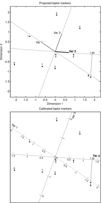
Clearly, to properly model the inner product defined in (2), (3) remains to be multiplied bykdjk. The projection in (3) can be done for all samplesiand to estimatexij they should all be multiplied by the same kdjk. Hence, the biplot interpretation is: (1) project the sample pointsci onto the vectorkdjkrepresenting variablejand (2) multiply this projection by the length of vectorj, that is, bykdjk. The multiplication by the variable’s vector length after the projection is a disadvantage of the biplot. The top panel of Figure 1 shows an example of the projection of sample 8 on variable 2. The projected estimatec0
8d2/kd2k= 1.89 which subsequently needs to be multiplied bykd2k=.70
to get the estimate 1.89×.70 = 1.32, which may be compared with the true data valuex82= 1.08.
Of course, this calculation has to be done mentally, using the visual information in Figure 1 giving the lengths of the projection and the length ofkd2k.
To eliminate this problem, Gower and Hand (1996) proposed using so called calibrated axes. In this approach, the lines representing the variables get marker points to indicate the predicted values. These calibrated marker points are obtained by dividing projected marker points by the lengthkdjk. Such a biplot with calibrated marker points is given in the bottom panel of Figure 1. Using calibrated marker points the estimated value can be read directly off the calibrated axes. The estimate of about 1.32 forx82is found by projection and interpolation between the markers 1
and 1.5. The arrows and edge scales are redundant and, therefore, not shown in the bottom panel of Figure 1.
-2 -1.5 -1 -0.5 0 0.5 1 1.5 2 -2 -1.5 -1 -0.5 0 0.5 1 1.5 2
Projected biplot markers
Dimension 1 Dimension 2 Var 1 Var 2 Var 3 1.89 1 2 3 4 5 6 7 8 9 -1.5
Calibrated biplot markers
-1 -0.5 0 0.5 1 1.5 -2 -1 0 1 2 Va r 1 1.5 1 0.5 -0.5 -1 -1.5 -2 2 Va r 3 1.32 1 2 3 4 5 6 7 8 9 Var 2
Figure 1: Example of projection in a biplot. Top panel shows only projection ignoring the length of the variable. In the bottom panel the length of the variables is taken into account by using calibrated biplot markers. In this case the value ofx82 is 1.08.
3
The PCA Area Biplot
The idea of the two-dimensional area biplot is very simple. One set of points (for example, the sample points) is rotated by 90◦. The estimate of the data value xij is obtained from the area
representation is superfluous and it suffices to represent variables as well as samples by points, each with a distinguishing plotting symbol. In each area biplot, no calibrated axes are needed nor post multiplication by the vector length of the variable. One relies on the ability of the eye to compare areas of different shaped triangles.
To develop the area biplot, letT be a 90◦ rotation matrix. The idea is to rotate the sample
points through 90◦, which does not change the length of a vector from the origin. The choice of
rotation by 90◦=π/2 follows from the equality
cos(θij) = sin(θij+π/2) = sin(φij),
where φij =θij+π/2 is the angle between the rotated sample point Tci and the variable vector
dj. Therefore, (2) can be expressed as
c0
idj=kcik kdjksin(φij).
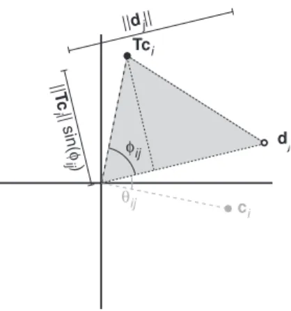
This may be immediately identified as twice the area of a triangle with sides kcik kdjk and angle φij but the following derives the result ab initio.
Figure 2 shows ci, dj, and the rotated versionTci. The part kTciksin(φij) is exactly that part of Tci orthogonal to dj, that is, the height of the shaded triangle. Therefore, the area of the triangle with heightkTciksin(φij) and basedj is exactlyc0idj/2 and this area estimates data valuexij/2.
As mentioned before, the standardization of C and Ddoes not affect the inner-products, or, equivalently, the areas. However, by using the typical PCA standardization whereC0C=Σ2 and D0D =I, the singular values are distributed over the row points. Hence, if there are relatively
many rows (a large sample) the row coordinates tend to become rather small compared to the column points. In such a configuration, drawing and comparing triangle areas may not be an easy task. For a visual inspection of triangle areas, it may be desirable that the row and column points exhibit a similar spread. In that way, the construction and comparison of triangles, which may have to be executed mentally, becomes much easier. To attain ”similar spread” we set
C=³n m ´1/4 U2Σ12/2 andD= ³m n ´1/4 V2Σ12/2.
It is then easily verified that the rows and columns ofCandDare standardized such thatC0C=
(n/m)1/2Σ
dj φij θij c i Tc i ||Tc i|| sin( φ ij) ||dj||
Figure 2: Triangle area interpretation of inner productc0
idj/2 through rotated sample pointTci.
is equal to (nm)−1/2Σ 2.
The rule for interpreting the data values from the area biplot is to construct a triangle as indicated above. Positive estimates of xij are obtained by areas that concur with rotation in a anti-clockwise direction starting from dj and negative estimates by a clockwise rotation. Zero areas occur wheneverdj andTci are on the same line through the origin. We note that all points through Tci parallel to dj generate the same area with dj, a result analogous to points on the circumference of a circle being equidistant from its center.
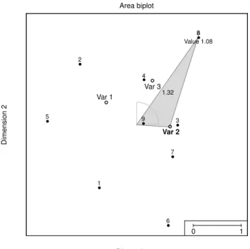
Figure 3 gives the example of the same random data ofn= 8 samples and p= 3 variables as shown in Figure 1. The solid black points indicate the 90◦ rotated samples CT0 and open circles
denote the variablesD. The shaded area belongs tox82as it is the triangle spanned by the origin,
variable 2, and sample 8. The area is 1.32 and is positive as the angleφ82 betweend2 andTc8 is
between 0 andπ. Any black pointTci below the line throughd2 has−π < φi2 <0, hence will
have negative estimates ofxi2.
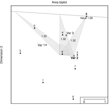
The shaded triangle in Figure 3 is not the only triangle with this area as there is a whole set of triangles with the same area. In Figure 4, two other triangles are added with the same area as the triangle in Figure 3 estimatingx82/2. All these triangles share the line from the origin tod2. The
third point can be chosen anywhere on the locus of points parallel to the line from the origin to
d2that goes through pointTc8. This property is useful for picking up values similar, in this case,
0 1 Area biplot Dimension 1 Dimension 2 Var 1 Var 2 Var 3 Value 1.08 1.32 1 2 3 4 5 6 7 8 9
Figure 3: Example of triangle area biplot. Solid circles represent the rotated sample points inCT0
and the open circles the variable points inD. The shaded area estimatesx82/2.
3.1
The Multidimensional Area Biplot
If one wants to visualize estimated values in more than two dimensions, the area biplot remains valid. To see this, note that thekdimensional inner product may be written as
c0d= k X j=1 cjdj = 2 X j=1 cjdj+ 4 X j=3 cjdj+...+ k X j=k−1 cjdj.
Hence, for an even number of dimensions, the inner-product can be factorized as the sum of two-dimensional inner-products. Then, by considering area biplots for subsequent pairs of dimensions, or, more precisely, by adding the areas in these plots, the multidimensional inner products are visualized. When plotting pairs of dimensions, care has to be taken to ensure that unit length is the same in all pairs; we refer to linked displays.
If an odd number of dimensions is chosen, a unidimensional area biplot is required to depict the contribution to the inner product for the dimension not contained in the two-dimensional biplots. It is not difficult to see that such a unidimensional area biplot can also be visualized as a two-dimensional area biplot. For the unidimensional case, the inner product simplifies intocikdjk. Hence, in a two dimensional display, these values can be represented by the sample vector [0 cik]0
Area biplot Dimension 1 Dimension 2 Var 1 Var 2 Var 3 Value 1.08 1.32 1.32 1.32 1 2 3 4 5 6 7 8 9 0 1
Figure 4: The three triangles have the same area all estimating x82/2.
[dj1 0]'
π/2
[ci10]
T[ci1 0]'
Figure 5: Unidimensional area biplot of inner productci1dj1through rotated sample pointT[ci10]0
and the variable vector [dj1 0].
rotated through 90◦ to positions along the vertical axis. As before, the productcikdjkis twice the
area of the triangle spanned by the origin, the sample point (0, cik), and the variable point (djk,0), see Figure 5. If the area is below the horizontal axis the estimated value is negative, if it is above the horizontal axis it is positive. A consequence of this is that for the same variable all estimated values span areas with the same base that only differ in height.
4
The Correspondence Analysis Area Biplot
Correspondence analysis (CA) analyzes association in an n×p two-way contingency table F. In particular, a bilinear decomposition is done on the deviations from the independence model. Although CA is ideally performed on a contingency table, computationally, the elements ofFmay contain any nonnegative values. To introduce the technical details, we need some notation. Let
Drdenote the diagonal matrix with the row sums ofFas elements,Dcis the diagonal matrix with the column sums ofFas elements, andsis the total sum ofF. Then, the independence model is given byE=Dr110Dc/s. CA can be expressed as minimizing
L(R,C) =kD−1/2
r (F−E−s−1DrRC0Dc)D−c1/2k2, (4)
where R and C aren×k andp×k matrices of row and column coordinates, respectively. The maximum dimensionality kis min(n, p)−1. For an exact solution to (4),RandC satisfy
s−1D1r/2RC0D1c/2 = D−r1/2(F−E)D−c1/2 i.e. RC0 = sD−1
r (F−E)D−c1.
Then, the inner products inRC0 estimate the elements
r0icj= fij−eij eij =
fij
eij −1, (5)
where r0
i is rowi ofR andc0j rowj of C. In other words, the inner products r0icj estimates the deviation of fij from independence relative to the estimated valueeij under independence. The ratiofij/eij is sometimes called the contingency ratio.
Approximations toRandC may be found from the SVD
s−1D1/2
r RC0D1c/2 = Dr−1/2(F−E)D−c1/2=UΣV0
giving
and
R = s1/2D−1/2
r UΣα
C = s1/2D−1/2
c VΣ1−α
for any scalar α. For α = 1 the so-called row principal normalization, for α = 0 the column principal normalization, and forα= 1/2 a symmetric normalization are obtained. All choices of αsimply distribute the singular valuesΣdifferently without changing the inner productr0
icj. The important part in the derivation above, lies in (5) as it indicates that in a CA biplot the elements estimated by the inner product approximate the relative deviations from independence. Therefore, we can apply the rotation straight away: choose a pair of dimensions of interest, for example, dimensions 1 and 2 and rotate the row points by 90◦. Then, the area of the triangle
spanned byTri,cj, and the origin estimates the contingency ratio minus one, that is,fij/eij−1.
5
Interaction Biplots
The biadditive model Y =µ110+α10+1β0+PK
k=1σkγkδ0k is often fitted to data given in an n×ptwo-way tableX, whereK= min(n, p). Here,αandβare usually termed main effects while the biadditive termsγkδ0
k represent interaction. This summation is parametrised in singular value decomposition form, see below. When fitted by least squares
b
α = X1/p−(np)−110X1and
b
β = X01/n−(np)−110X1,
where 1 is a vector of ones of conformable length. The biadditive term is estimated by first calculating the deviations from the main effects: Z = (I−P)X(I−Q) where P = 110/n and Q=110/p. The biadditive terms are estimated from the singular value decomposition ofZ. It is
well known that if the singular values σk are represented in nonincreasing order then the first k terms in the summation gives the best k-dimensional representation of the interaction. In many (most) practical situations we are concerned with the case ofk= 2 and with visualization in two dimensions obtained by plotting the nrows of the n×2 matrix (c1,c2) for row points and the p
rows of the p×2 matrix (d1,d2) for column points.
re-spectively. By rotating one set of points by 90◦, the new biplot may be used to visualise the
approximation to the interactions.
6
Examples
To show how the area biplot can be applied in practice we give two examples. In the first example, we use a PCA area biplot whereas the second example concerns a CA area biplot.
6.1
PCA area biplot: Alcohol consumption in Japan
We apply the area biplot to 1994 data on alcohol consumption in Japan. The data are obtained from the websitehttp://mo161.soci.ous.ac.jp/@d/DoDStat/DataList/index.html. For each of the 46 prefectures, the total consumption, in Japanese Yen, for 5 popular alcoholic beverages is recorded. The beverages are: beer, sake (a traditional Japanese rice wine), shouchuu (a traditional Japanese distilled alcoholic beverage), whiskey and wine. To eliminate the effect of the size of prefectures, the original figures are divided by the number of inhabitants per prefecture. These data are reported in Table 1 together with theirz-scores.
To analyze the variations of alcohol we apply PCA to thez-scores and obtain a two-dimensional biplot. This two-dimensional solution accounts for approximately 68% of the total variation.
Figure 6 shows the area biplot where the prefectures are represented by solid dots and the alcoholic beverages by open dots. At the left bottom of the plot we find the prefectures Miyazaki and Kagoshima. These are prefectures located in the Southwestern part of Japan on the Kyushu island. It is clear that the triangles corresponding to the wine consumption have a surface close to zero for these prefectures. Also, the triangles formed with shouchuu and sake will be relatively large and comparable in size. For Kagoshima, the area corresponding to shouchuu consumption is 2.46 and the area for sake consumption is 2.75. However, the sign corresponding to the estimated inner products differs for these two beverages: it is positive for shouchuu and negative for sake. Hence, the estimated z-scores for shouchuu and sake consumption in Kagoshima, are 2.46 and -2.75 respectively. Similarly, we can obtain the estimated values for Miyazaki which are 2.53 and -2.56. Clearly, in these prefectures the estimated consumption of shouchuu is considerably larger than average whereas the estimated consumption of sake is considerably smaller than the average sake consumption. Note that these estimated values are in accordance with the z-scores in Table 1. The Kyushu island is particularly famous for its shouchuu production which explains the higher consumption for these prefectures. Moreover, according to the entry for Kagoshima in
Table 1: Average alcohol consumption per Japanese prefecture for five types of alcohol.
Average per inhabitant z-scores of average per inhabitant
Prefecture Sake Shochu Bear Wine Whisky Sake Bear Wine Whisky
Aichi 8.63 2.67 56.89 1.08 1.11 -0.63 -0.75 0.76 -0.06 -0.28 Akita 20.31 5.25 57.09 1.04 1.77 2.28 -0.07 0.79 -0.10 1.31 Aomori 11.71 7.80 56.36 1.20 2.12 0.14 0.60 0.69 0.11 2.17 Chiba 7.15 5.56 40.52 1.10 1.02 -1.00 0.01 -1.52 -0.03 -0.50 Ehime 10.99 4.08 52.73 0.67 0.94 -0.04 -0.38 0.18 -0.60 -0.69 Fukui 13.31 1.57 56.51 0.62 1.07 0.54 -1.03 0.71 -0.66 -0.39 Fukuoka 8.55 7.10 52.87 1.05 1.21 -0.65 0.41 0.20 -0.09 -0.03 Fukushima 14.58 5.25 47.07 0.89 1.79 0.85 -0.07 -0.61 -0.31 1.37 Gifu 11.65 2.09 49.13 0.73 0.87 0.12 -0.90 -0.32 -0.52 -0.86 Gunma 9.63 7.80 44.02 1.07 0.92 -0.38 0.60 -1.03 -0.06 -0.76 Hiroshima 10.97 4.68 59.14 1.09 1.25 -0.05 -0.22 1.08 -0.03 0.07 Hokkaido 8.18 8.91 55.48 1.85 1.72 -0.74 0.89 0.57 0.95 1.19 Hyogo 9.23 2.35 51.86 0.99 1.21 -0.48 -0.83 0.06 -0.17 -0.05 Ibaragi 9.88 5.06 42.50 0.81 1.01 -0.32 -0.12 -1.25 -0.40 -0.53 Ishikawa 15.62 1.74 58.01 0.89 1.19 1.11 -0.99 0.92 -0.31 -0.10 Iwate 12.09 7.22 47.88 1.03 1.32 0.23 0.44 -0.49 -0.12 0.23 Kagawa 10.91 2.92 51.04 0.81 1.05 -0.06 -0.68 -0.05 -0.41 -0.44 Kagoshima 1.36 18.42 44.68 0.54 0.47 -2.44 3.38 -0.94 -0.76 -1.85 Kanagawa 7.55 5.96 46.92 1.51 1.65 -0.90 0.12 -0.63 0.51 1.04 Kochi 13.95 4.02 66.53 0.76 1.37 0.70 -0.39 2.11 -0.47 0.35 Kumamoto 5.01 11.76 50.60 0.74 0.68 -1.53 1.63 -0.11 -0.50 -1.34 Kyoto 10.24 2.01 56.96 1.33 1.27 -0.23 -0.92 0.77 0.27 0.10 Mie 10.79 2.63 45.65 0.68 1.00 -0.09 -0.76 -0.80 -0.58 -0.56 Miyagi 11.78 4.98 46.44 1.19 2.13 0.16 -0.14 -0.69 0.10 2.21 Miyazaki 2.79 19.93 49.66 0.81 0.64 -2.09 3.78 -0.24 -0.41 -1.42 Nagano 14.30 5.58 49.29 1.80 1.12 0.78 0.01 -0.30 0.89 -0.27 Nagasaki 9.25 7.93 50.44 0.77 1.09 -0.47 0.63 -0.14 -0.46 -0.32 Nara 7.81 1.65 43.69 0.63 0.71 -0.83 -1.02 -1.08 -0.64 -1.27 Niigata 24.43 2.83 60.14 1.17 1.50 3.31 -0.70 1.22 0.07 0.67 Oita 8.30 11.76 48.49 0.86 1.61 -0.71 1.64 -0.41 -0.34 0.93 Okayama 11.31 3.73 46.02 0.77 1.03 0.04 -0.47 -0.75 -0.46 -0.48 Osaka 9.49 2.92 71.21 1.52 1.69 -0.42 -0.68 2.76 0.53 1.14 Saga 12.89 5.07 49.46 0.60 0.81 0.43 -0.12 -0.27 -0.68 -1.02 Saitama 7.20 5.94 41.09 1.08 1.04 -0.99 0.11 -1.44 -0.05 -0.45 Shiga 10.84 1.96 42.15 0.71 0.87 -0.08 -0.93 -1.29 -0.54 -0.87 Shimane 16.96 5.46 51.41 1.64 0.99 1.45 -0.02 -0.00 0.68 -0.58 Shizuoka 10.25 6.00 47.66 1.16 1.14 -0.23 0.13 -0.52 0.06 -0.22 Tochigi 9.64 5.33 42.29 0.78 1.00 -0.38 -0.05 -1.27 -0.45 -0.56 Tokushima 10.88 2.76 47.94 0.61 0.92 -0.07 -0.72 -0.48 -0.67 -0.74 Tokyo 10.59 7.16 71.14 3.49 2.39 -0.14 0.43 2.75 3.10 2.83 Tottori 15.32 3.19 53.31 0.78 1.20 1.04 -0.61 0.26 -0.45 -0.06 Toyama 16.20 1.81 54.47 0.80 1.15 1.26 -0.97 0.43 -0.43 -0.18 Wakayama 13.45 2.17 59.04 0.69 1.22 0.57 -0.88 1.06 -0.56 -0.03 Yamagata 16.53 4.88 49.14 1.37 1.98 1.34 -0.17 -0.32 0.33 1.84 Yamaguchi 10.92 6.50 57.23 0.75 1.25 -0.06 0.26 0.81 -0.48 0.06 Yamanashi 9.73 7.50 42.97 5.08 0.93 -0.35 0.52 -1.18 5.19 -0.71
the Wikipedia, Kagoshima is the only prefecture in Japan that does not produce sake. Opposite Kagoshima and Miyazaki, we find Niigata and Akita. These prefectures are famous for their sake. This reflects itself in the plot as the triangle with the origin and sake is relatively large, and the sign of the estimated inner product is positive.
On the top left of the plot we find Tokyo prefecture which comprises the Tokyo metropoli-tan area. Making the triangles we immediately see that Tokyo is the only prefecture where the estimated consumption is higher than average for all beverages. In particular, whiskey (with an
Area biplot Dimension 1 Dimension 2 Sake Shouchuu Beer Wine Whisky Akita Aomori Hokkaido Kagoshima Kumamoto Miyazaki Nara Niigata Osaka Tokyo Yamanashi O 0 1
Figure 6: Area biplot for average expenditure on alcohol consumption in 46 Japanese prefectures (solid dots, some with label) on 5 types of alcohol (open dots and labels).
estimatedz-score equal to 3.01), wine (3.09) and beer (2.27) show much higher levels of estimated consumption than in the rest of the country. Again, comparing the estimated values to the data values in Table 1, we see that the approximation is quite reasonable.
Finally, Yamanashi prefecture, in the plot located on the far left side, appears to have a some-what unique position that indicates a relatively high estimated consumption of wine. The estimated value is 2.06. The reason for this may be the fact that Yamanashi, which is located directly to the west of Tokyo and in which mount Fuji is located, is the country’s top producer of wine. Note that, thez-score for wine consumption in Yamanashi is 5.19. Hence, the estimated value underestimates this score quite significantly.
We can interpret the levels of consumption of the alcoholic beverages for other prefectures in a similar fashion.
6.2
CA area biplot: Seat distribution in the European parliament
(hy-pothetical data)
In Table 2, a hypothetical data set is presented concerning the distribution of seats in the Euro-pean parliament (Borg & Groenen, 2005). As this table has only three columns, the maximum dimensionality is 2. Figure 7 shows the corresponding exact area biplot using the symmetric
stan-Area biplot Dimension 1 Dimension 2 Christ. Dem. Socialists Other -0.22 -0.52 0.94 Belgium Germany Italy Luxembourg The Netherlands 0 0.5
Figure 7: Area biplot for correspondence analysis.
dardization of α=.5. Note that the relative distributions of the seats over the political factions are the same for Germany and The Netherlands, so that these points are superimposed in the biplot as is required by CA. The last three columns of Table 2 give the relative deviation from independence that is estimated by the area in the area biplot. The table shows that Italy deviates most from independence. This observation is reflected in the shaded areas of Italy with each of the political factions: the positive area of .94 for the Other faction indicates that Italy is relatively more represented by the Other faction and less by the socialists (a negative area of−.52) and the Christian democrats (area is−.22).
Table 2: A contingency table of the distributions of seats by country and political faction (hypo-thetical data) (Borg & Groenen, 2005).
Frequencyfij (fij−eij)/eij
Country CD Soc Other Total CD Soc Other
Belgium 8 9 7 24 -0.22 0.24 0.09 Germany 39 30 6 75 0.21 0.32 -0.70 Italy 25 11 39 75 -0.22 -0.52 0.94 Luxembourg 3 2 1 6 0.16 0.10 -0.38 The Netherlands 13 10 2 25 0.21 0.32 -0.70 Total 88 62 55 205
7
Conclusion and Discussion
The area biplot can be used for any model that has a biadditive component. Here it is shown how the area biplot can be used in principal components analysis, correspondence analysis, and biadditive models. In all three cases, the area spanned by a triangle between the origin, row point i, and column point j estimates the data value ij. In PCA, this happens directly, in CA the estimate approximates the contingency ratio minus one, and in the biadditive model, it estimates the deviation from the main effects.
The idea of using area to estimate data values comes up naturally in the singular value de-composition of skew-symmetric matrices (Gower, 1977; Constantine & Gower, 1978). There, the singular values come in equal pairs with corresponding left and right singular vectors. Instead of plotting both right and left singular vectors and interpreting the inner products, only one pair (hedron) of dimensions of the left (or right) singular vectors is used to plot npoints. Similar ge-ometry then applies to that discussed in Section 3. The area of triangles generated by theith and jth points and the origin estimation the corresponding data value in the skew symmetric matrix.
PCA is often explained as the eigendecomposition of a correlation matrix. The resulting plot of a single et of points representing the component loadings of the variables gives inner product estimates of the correlation between pairs of variables. In this case, too, the area representation in two dimensions is available but to obtain the second set of points, the first set has to be rotated through 90◦. Thus, the number of points to be represented is doubled, which could be seen as too
high a price to pay.
We have seen that area biplots may be used to represent any number of dimensions, odd or even. Hence, provided some convenient way is available for evaluating the two-dimensional inner-products, as in the area biplot, a visual approximation of several dimensions is available. The areas in successive pairs of dimensions have only to be added, requiring care in the compatible scaling of linked two-dimensional plots. Of course, as a visual process, this loses credibility as the number of dimensions increases. These remarks draw attention to the common practise of plotting all pairs of dimensions which seems unnecessary when inner products are the vehicle of interpretation. When distance interpretations are required, our approach is not available but mentally combining two or more distance maps requires distances in each pair of dimensions to be squared, added and then “square-rooted” which seems to us to be beyond reasonable demands.
References
Borg, I., & Groenen, P. J. F. (2005). Modern multidimensional scaling: Theory and applications
(2nd edition). New York: Springer.
Constantine, A. G., & Gower, J. C. (1978). Graphic representations of asymmetric matrices.
Applied Statistics,27, 297–304.
Gabriel, K. R. (1971). The biplot-graphic display of matrices with applications to principal components analysis. Biometrika,58, 453–467.
Gower, J. C. (1966). Some distance properties of latent root and vector methods used in multi-variate analysis. Biometrika,53, 325–338.
Gower, J. C. (1977). The analysis of asymmetry and orthogonality. In F. Brodeau, G. Romier, & B. Van Cutsem (Eds.), Recent developments in statistics (pp. 109–123). Amsterdam: North-Holland.