Metropolia University of Applied Sciences Master of Engineering
Information Technology Master’s Thesis
5 June 2020
Muhammad Arshad Haroon
ECG Arrhythmia classification using Deep Convolution
Neural Networks in Transfer Learning
Author Title
Number of Pages Date
Muhammad Arshad Haroon
ECG Arrhythmia classification using Deep Convolution Neural Networks in Transfer Learning
47 pages 5 June 2020
Degree Master of Engineering
Degree Programme Information Technology
Instructor Sami Sainio, Principal Lecturer Metropolia UAS
Electrocardiogram (ECG) is a health monitoring test which assists clinicians to detect abnormal cardiac activity based on heart’s electrical activity. Early classification of ECG signals is important towards the possible treatment measures for the patients. In principle ECG is a time series signal as a result of heart’s electrical activity. Various methods have been devised to apply Machine learning algorithms for the classification of these time series signals. These methods require feature extraction which in turn pose problems such as inconsistency in the extracted features as well as variability found in the ECG features. Deep learning methods such as algorithms based on Convolution Neural Networks (CNN) can be used to avoid manual crafting of features from ECG signals. Due to the large amount of ECG data and the complexity of CNNs, GPU processing is often required in order to train and test the models quickly. Google Colab provides a free tier with limited memory space for implementing complex and deep neural networks. Also, already trained network on some other data can be used to learn common features for new data and modified to produce desired results. Among many, ResNet-50 and VGG-16 are well-known models being used for transfer learning.
In this project study ECG data is acquired from MIT-BIH Arrhythmia database. Using wave form database (wfdb) library in Python ECG signals were studied and observations were made for different characteristics and data variations. QRS detection was performed by locating the R peaks in ECG strips based on the annotation files for individual records. Segmented one dimen-sional data was converted to images for deep neural network training via CNN. Multilayer CNN, ResNet-50 and VGG-16 were used for deep convolution and transfer learning and the computing was performed in Google Colab environment. Accuracies of 83 % via ResNet-50 and 99 % via VGG-16 were achieved using two dimensional ECG data. Higher accuracy with VGG-16 proves that Transfer learning can be applied for ECG arrhythmia classification.
Keywords Electrocardiogram, Machine Learning, Feature Extraction, Deep Learning, Transfer Learning, Arrhythmia
Contents Abstract List of Figures List of Tables List of Abbreviations 1 Introduction 1
1.1 Electrocardiography and ECG 1
1.2 Pre-processing of data 3
1.3 Classification 4
1.4 Neural network 5
1.5 Convolution neural networks 6
1.5.1 Activation function 8
1.5.2 Pooling layers 8
1.5.3 Fully connected layer and Softmax activation 9
1.5.4 Dropout and Flatten layers 9
1.5.5 Back propagation and Gradient descent 10 1.6 Transfer learning with Deep Convolution neural network 11
1.6.1 ResNet-50 residual network 12
1.6.2 VGG-16 model 12
2 Literature Survey 14
2.1 LSTM network model 14
2.2 Adaptive Convolution neural network 15
2.3 Deep Convolution neural network and PTB 15
2.4 Deep Convolution neural network and Categorical classification 17
2.5 Transfer learning 18
2.6 Other Machine learning methods 19
2.7 Transfer learning efficiency parameters 19
2.8 ResNet work on MIT-BIH and PTB datasets 20
2.9 VGG-16 and Breast cancer image model 21
3 Current State Analysis 22
4 Material and Methods 23
4.1 Database 23
4.2 Preprocessing 25
4.3 Image processing and Encoding 27
4.4 Overfitting and Data augmentation 28
4.5 Convolution neural network and classification 28
4.5.1 CNN models 28
4.5.2 Transfer learning 30
4.7 Neural network configuration 32 5 Results 33 5.1 Binary classification 34 5.2 Categorial classification 36 5.3 Classification via VGG-16 38 5.4 Discussion 39 References 42
List of Figures
Figure 1-1 Cardiovascular diseases and their effect on different regions around the world (Aje, T., 2009) .. 1
Figure 1-2 Cardiac cycle in an ECG ... 2
Figure 1-3 Types of arrhythmia and Normal ECG signal (Sahoo, S et al. 2020) ... 3
Figure 1-4 Types of noise and its presence in an ECG strip (Sahoo, S et al. 2020) ... 4
Figure 1-5 Machine learning and Deep learning difference ... 5
Figure 1-6 A simple neural network ... 6
Figure 1-7 Feature value extraction in CNN ... 7
Figure 1-8 ReLu activation function ... 8
Figure 1-9 Max pooling on convolution layer ... 9
Figure 1-10 A full sequence of a CNN with fully connected and softmax layers for output ... 10
Figure 1-11 (a)Machine learning vs (b)Transfer learning ... 11
Figure 1-12 Error value decrease in ResNet-50 (right) in comparison with plain Machine learning model (left) (Abrol, A. et al., 2020) ... 12
Figure 1-13 Detailed architecture of a VGG-16 CNN model ... 13
Figure 2-1 Segmented Normal and Myocardial infarction ECG signals (Oh, S. et al. 2018) ... 16
Figure 2-2 Graphical spread of three different beats data on training and validation sets (Isin, A. and Ozdalili, S., 2017) ... 18
Figure 2-3 Block view from data acquisition to classification (Isin, A. and Ozdalili, S., 2017) ... 18
Figure 2-4 transfer learning from source to target feature space (Zhang, L., 2020) ... 20
Figure 2-5 ResNet basic architecture ... 20
Figure 4-1 ECG signals from two leads. Upper blue signal from Lead II, Lower orange signal is from Lead VI ... 23
Figure 4-2 An extracted ECG signal from two leads ... 24
Figure 4-3 Lead II ECG signal ... 24
Figure 4-4 R peak detection in an ECG strip and segmentation ... 25
Figure 4-5 Extraction of normal and arrhythmia ECG beats as images ... 26
Figure 4-6 Normal, PVC, Paced, RBBB and LBBB ECG beats ... 26
Figure 4-7 Result of data augmentation of an input image ... 28
Figure 4-8 CNN model for binary classification of Normal and PVC beats ... 29
Figure 4-9 CNN model for 3 and 5 categories ECG data classification ... 30
Figure 4-10 ResNet-50 architecture for binary classification ... 31
Figure 5-1 Accuracy and Loss values for binary classification of Normal and PVC beats ... 35
Figure 5-2 Binary classification of Normal and PVC beats using ResNet-50 ... 35
Figure 5-3 Accuracy and loss values for categorical classification of Normal, PVC and Paced ECG beats37 Figure 5-4 Accuracy and loss values for categorical classification of Normal, PVC, LBBB, RBBB and Paced ECG beats ... 37
Figure 5-5 Classification of Normal, PVC, LBBB, RBBB and Paced ECG beats using VGG-16 CNN ... 38
List of Tables
Table 2-1 Normal and Myocardial Infarction statistical data (Oh, S. et al. 2018) ... 16
Table 2-2 Categorical division of ECG beats into 5 classes (Acharya, U. et al., 2017) ... 17
Table 2-3 CNN layers and kernel size information for each layer (Acharya, U. et al., 2017) ... 17
Table 4-1 Summary of ECG records extraction as images ... 27
Table 4-2 Categorical encoding of ECG beats ... 27
Table 5-1 Statistical information of ECG data extraction from MIT-BIH arrhythmia database ... 33
Table 5-2 Normal and PVC ECG beats for classification ... 33
Table 5-3 Normal, PVC and Paced beats for classification ... 34
Table 5-4 Input data for 5 classes classification ... 34
Table 5-5 Binary classification label encoding (group 1) ... 34
Table 5-6 Accuracy of binary classification ... 35
Table 5-7 3 classes ECG beats label encoding (group 2) ... 36
Table 5-8 5 classes ECG beats label encoding (group 3) ... 36
List of Abbreviations
AF Atrial Fibrillation
CAE Convolutional Auto-Encoder CNN Convolution Neural Network
GPU Graphical Processing Unit
LBBB Left Bundle Branch Block LSTM Long-Short Term Memory MI Myocardial Infarction (MI) NSR Normal Sinus Rhythm
PAC Premature Atrial Contractions
PTB Physikalisch-Technische Bundesanstalt PVC Premature Ventricular Contractions RBBB Right Bundle Branch Block
ReLU Rectified Linear Unit
VF Ventricular Fibrillation VT Ventricular Tachycardia WFDB Wave Form DataBase
1 Introduction
Healthy circulatory system of blood through heart’s regular contractions is very important to human health. Heart pumps the blood to body through arteries and any blockage of arteries can lead to possibly fatal heart stroke (Aje and Miller, 2009), (Moore et al. 2013), (Sahoo, S et al., 2020). Some of the biggest causes behind the occurrence of coronary heart diseases are smoking, diabetes, hypertension, obesity as well as uncommon fac-tors such as HIV/AIDS, vitamin D and B12 deficiencies and other physiological factors (Aje, T., 2009). Cardiac diseases are one of the biggest threats that human life faces. About 31 % deaths in the world are caused by cardiovascular diseases (Sahoo, S et al., 2020). Figure. 1-1 shows that the top reason of deaths in almost all the regions of the world is due to heart diseases.
Figure 1-1 Cardiovascular diseases and their effect on different regions around the world (Aje, T., 2009)
1.1 Electrocardiography and ECG
Early recognition of a cardiac disease is very important since heart disease can lead to instant death (Li, Y. and Cui, W., 2019). Electrocardiogram (ECG) is a detailed and noninvasive test containing powerful information useful in finding treatments for heart
diseases (Jaeger, 2010), (Sahoo, S et al., 2020), (Li, Y. and Cui, W., 2019). Electrocar-diography is a method of monitoring the potential differences on human skin that are caused by depolarization and repolarization of the heart muscles. Generally, ECG data is acquired via Limb leads. Limb leads are used for measuring the electrical activity in human body (Goldberger et al. 2003). The resulting information package is called an ECG (Levick, J., 1991). ECG record is a waveform consist of many different waves and peaks. A usual ECG record contains a P wave, QRS section and a following T wave per cardiac sequence (Tse, 2016), (Van, 2004), (Jaeger, 2010), (Sahoo, S et al., 2020). Fig-ure. 1-2 shows a normal cardiac cycle.
Figure 1-2 Cardiac cycle in an ECG
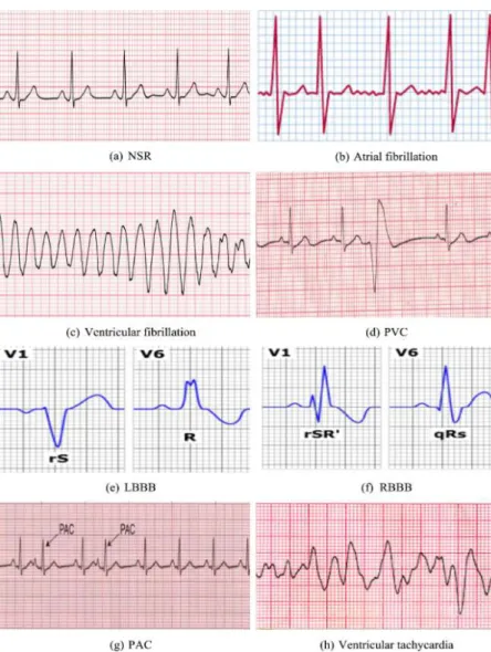
A QRS complex is the focus of the ECG recordings and any abnormal heart activity can be noticed by observing the structure of the ECG segment containing the QRS complex. Irregular sequence of QRS and its surrounding waves reflect the presence of abnormal heart activity called arrhythmias (Van et al., 2004), (Tse, 2016), (Sahoo, S et al., 2020). Some of the common arrhythmia that can be found in some ECG recordings along with (a) Normal sinus rhythm (NSR) are (b) Atrial fibrillation (AF), (c) Ventricular fibrillation (VF), (d) Premature ventricular contractions (PVCs), (e) Right bundle branch block (RBBB), (f) Left bundle branch block (LBBB), (g) premature atrial contractions (PAC) and (h) Ventricular tachycardia (VT) as shows in Figure. 1-3 (Sahoo, S et al., 2020).
1.2 Pre-processing of data
Usually an acquired ECG signal contains a lot of extra information in the form of noise. This noise can be of different types. Figure. 1-4 (Sahoo, S et al. 2020) shows the pres-ence of different noise signals in an ECG data strip. This extra information on ECG signal is usually useless during the interpretation of the cardiac cycles (Yeha and Wang, 2008), (Friesen et al., 1990), (Sahoo, S et al. 2020). Adequate preprocessing of the ECG signals is required before heading towards the more detailed examinations of the structures of the strips. Averaging and adaptive filters are some of the examples of preprocessing methods used for the noise removal from an ECG data strip.
Figure 1-3 Types of arrhythmia and Normal ECG signal (Sahoo, S et al. 2020)
Figure 1-4 Types of noise and its presence in an ECG strip (Sahoo, S et al. 2020)
1.3 Classification
After preprocessing, ECG data can be further examined to observe the normal and ir-regular cardiac activities. In order to accurately detect arrhythmia automatically, different methods are being used for the last four decades (Yeha and Wang, 2008), (Sahoo, S et al., 2020). These methods can be categorized as supervised and unsupervised learning techniques. Some of these techniques are discrete wavelet transform (Diker, A. et al., 2019), machine learning model (Chang, K. et al., 2020), spectral correlation and support vector machines (Khalaf, A. et al., 2015), parameterization approach (Liu, B. et. Al 2015), Empirical Mode Decomposition (E. Izci et al., 2018), Spectrogram and Convolutional Neural Network (CNN) (J. Huang et. al 2019) and 1-D CNN (Ç. Sarvan and N. Özkurt, 2019).
It is noticeable that most of the approaches for the detection of arrhythmia use machine leaning methodologies. Kononenko (2001) describes the use of machine learning meth-ods because of their strong requirements criteria such as higher desirable performances over other techniques, ability to deal with missing and noisy data, capacity to present explanation for the observers while requiring fewer tests. Machine Learning algorithms
are mainly categorized as supervised learning and unsupervised learning methods (Brownlee, J., 2019). Machine learning methods require feature extraction from the data in order to do proper classification and detection. A modified approach of machine learn-ing is deep learnlearn-ing where the intermediate step of human assisted feature extraction is skipped (Brownlee, J., 2019). Instead the leaning algorithm learns the features automat-ically from the original data (Rahhal, M. et. al 2016). Figure. 1-5 presents the difference between machine learning and deep learning methodologies.
Figure 1-5 Machine learning and Deep learning difference
1.4 Neural network
A simple neural network that is used for training input data to classify output values is presented in Figure 1-6. Neural networks have three types of layers. An Input layer that takes in the input values, hidden layers that apply the weights of the layers to the input data by using an activation function to decide on output values and an output layer that generates the results (Gurney, 1997).
Figure 1-6 A simple neural network
Here I1, I2, I3 are the input values from a data set. W11, W12….W33, Wxy are the weights
(magnitude values) of the connections between nodes of the layers and
f
represents the activation functions that generate the results at hidden (here H1, H2) and outputlayer(here R) using a criteria. Weights determine the strength of a link between nodes. If weights are higher than the input connected to it has a higher impact on the output. A lower value closer to zero means the input will not have much effect on the output nodes.
b
represents the bias in the network for a neuron. Bias is a constant value that is used to adjust the output for the weighted sum of inputs. When an output is generated in the forward moving direction, usually it lacks accuracy in first iteration. The output response is then back propagated to adjust the weights in order to improve the learning process by getting the right output in next forward iterations. In practice training data properties such as values and types may vary in a dataset. Therefore, input for Neural networks are generally normalized on a fixed scale at input layer. For example, Age and height in a population dataset are originally on two different scales due to their natural value dis-tribution but after normalization on a standard scale between 0 and 1, there values will always be between 0 and 1. Normalized input features increase the neural network learn-ing rate.1.5 Convolution neural networks
This thesis work is based on classifying various data categories by means of training and learning neural networks. CNN based classification models have been used in the cur-rent study for the classification purposes. In general, CNNs consist of convolution and pooling stages that help getting the meaningful features out of the image maps (Mebsout,
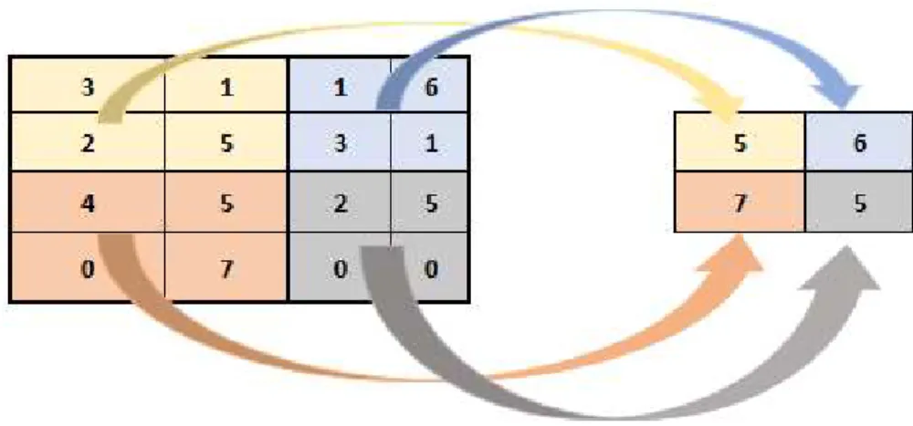
I., 2020). A CNN model uses input in the form of a three dimensional tensor i.e. An image with its width and height information and an RGB (Red, Green and Blue channels) value. This input image then proceeds with the stages of further processing in the neural net-work. These steps are called layers of the network (Wu, J., 2017). The process of convo-lution starts by placing a kernel (usually a 2 x 2 or 3 x 3 matrix as filter) over a region in the image map. Usually this region is the first pixels on top left portion of image matrix that fits the kernel size. Pairwise multiplication of image and kernel pixel values is summed up for a final value in feature map (a modified version of image matrix). Figure 1-7 shows the calculation of first pixel value in Feature map from input image of 6 x 6
and a kernel size of 3 x 3. Similarly, all values are calculated as the new feature value set.
Figure 1-7 Feature value extraction in CNN
This kernel is moved on image data from left to right in step increments of 1. These step increments are called strides. The stride value for this convolution is 1. The convolution
F
of a kernel and image data is represented by the following equation (Skalski, P., 2019).𝐹(𝑖, 𝑗) = ∑ ∑ 𝐾(𝑚, 𝑛) ⋅ 𝐼(𝑖 − 𝑚, 𝑗 − 𝑛)
(1)
Where
I
is the input image with dimensionsi
andj
,K is the kernel of size
m
xn
andF
( i , j )
is the output convolution matrix. In practice most CNN models contain activation functions, pooling layers, fully connected layers, dropout, flatten and output layers. For this thesis work CNN models contained all the above-mentioned layers in various ar-rangements.1.5.1 Activation function
Every Convolution layer in CNN model is usually followed by an activation function. One common choice for most CNN models is ReLu (Rectified Linear Unit) function. ReLu sets the negative values of input feature matrix as zero (Ujjwalkarn, U., 2016). CNNs are used mostly for real world information processing and therefore nonlinearity in the learning model is needed as convolution itself lies in the group of linear operations (Ujjwalkarn, U., 2016). Mathematically ReLu is defined as
𝑓(𝑥) = 𝑚𝑎𝑥 (0, 𝑥)
(2)
Above equation computes ReLu,
f(x)
to generate zero output values for all the negative entries of inputx
and identity otherwise. Figure 1-8 shows ReLu activation function.Figure 1-8 ReLu activation function
1.5.2 Pooling layers
Adding pooling layers in CNN after convolution layers decrease the spatial dimensions of the feature maps i.e. the resultant matrix has less dimensions with more meaningful features. Figure 1-9 shows, how a 4 x 4 matrix is converted to a feature value set of 2 x 2. Pooling layers help reduce the number of parameters in the network and therefore assist in avoiding over fitting problems. Overfitting in CNN based models happen when the neural network gets trained on original details as well as noise information, hence leading to a negative effect on classification (Brownlee, J., 2016). Even though pooling layers reduce the size of the feature maps, they can keep the most signification infor-mation for further processing of data in the network. For current thesis work Max pooling
operation is selected for pooling steps, where a 2 x 2 window is used in the similar man-ner as shown in Figure 1-9. Here the maximum of every set is selected as a feature input towards the feature value set.
Figure 1-9 Max pooling on convolution layer
1.5.3 Fully connected layer and Softmax activation
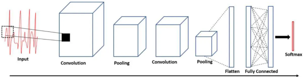
Feature map with most significant information extracted from convolution and pooling layers are used in fully connected layers where each node (neurons in neural network) in the adjacent layers are connected to neurons in the next layers. Full connected layers are sometimes called dense layers. Fully connected layers use the extracted features from previous layers to perform early classification on input data (Ujjwalkarn, U., 2016). Figure 1-10 shows the fully connected and softmax layers in the architecture of CNN. Softmax activation layer is used to finally classify the training data classes.
1.5.4 Dropout and Flatten layers
Dropout layers are used to drop some information on some of the neurons in the network to avoid over fitting problems (Srivastava et al., 2014), whereas flatten layers are used before output layer to convert multidimensional output into a vector (Brownlee, 2018). This step is necessary to get the output shape according to the number of classes trained and predicted. For example, if training on a CNN, the input data consisted of two cate-gories then the flatten layer is needed to reduce the fully connected layer’s result to a
vector of 2 values. One for each category. Similarly, a larger vector is generated for more categorical information classification at the output layer.
Figure 1-10 A full sequence of a CNN with fully connected and softmax layers for output
1.5.5 Back propagation and Gradient descent
In principle a CNN model takes image data and carries it through steps of forward prop-agation from convolution layers to fully connected layers. Output values are then calcu-lated for training data classes. During the first iteration, weights are given randomly there-fore output values are also random. At this stage the error is calculated and backpropa-gated by calculating its gradients using weights in previous layers of the CNN network. Parameters of the CNN models are then updated by gradient descent (Ujjwalkarn, U., 2016). Gradient descent is a method of minimizing some function values by moving to-wards the local minimum value.
During the process of classification, the predictions are made when the input data is trained via neural network. A network prediction accuracy can be represented by
p
and a desired accuracy byy
. Thus, forS
set of predictions if the network value of predictionis
p
and the desired target values arey
then the Error can be calculated as𝐸 = ∑ (𝑦 − 𝑝)
(3)
Using back propagation, this error values is reduced by changing the weights in a way that
p
andy
values are close to each other. In back propagation this is achieved by altering the values of weights with respect to the gradient descent methods. Using thesemethods partial derivatives of the weight (
W
) values are calculated with respect to error (E
) values as following.𝜕𝐸
𝜕𝑊𝑥, 𝑦
1.6 Transfer learning with Deep Convolution neural network
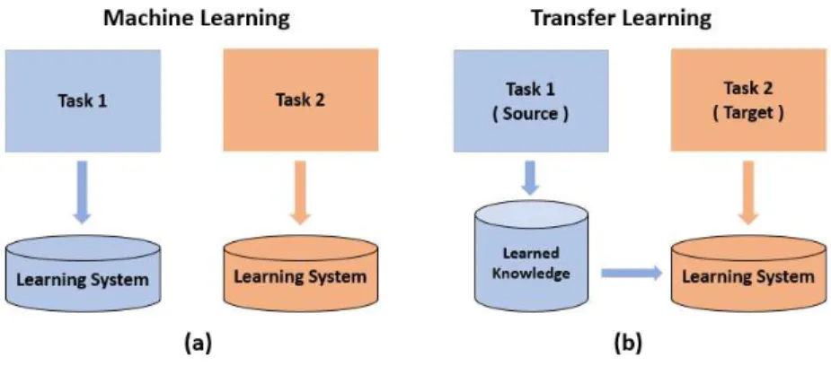
Although traditional CNNs are used in the initial implementations of this research study, a more modern approach of using CNN called transfer learning is also focused for com-puting classification accuracies. Conventionally machine learning and deep learning models and their respective training and validation datasets must be in the same feature space and must have the same distribution, however since 2005 a new approach ‘trans-fer learning’ presents a completely new perspective of learning (S. J. Pan and Q. Yang, 2010). In transfer learning approach knowledge of one data set learning can be utilized for a different related dataset. Usually transfer learning models can be utilized in two ways. One is to use the fully trained network on new data and the other method is to use some of the layers of the pre trained network as trainable and then tuning those layers to achieve desired accuracies. Figure 1-11 presents the difference between traditional machine learning models and the transfer learning approach. Some of the well-known models for using transfer learning are ResNet-50 and VGG-16. Both these models are CNN based.
1.6.1 ResNet-50 residual network
Even though the deep learning models (multiple layers) result in promising output, yet there is the issue of more layers resulting in more loss which means at some point deeper networks will present less training accuracy. Fortunately, deep residual learning answers the above-mentioned complexity issues. In residual learning a network output does not only learn from the activation of previous layer but also from the original input to that preceding layer (Abrol, A. et al., 2020). Some examples of common residual deep learn-ing network are ResNet-18, ResNet-34 and ResNet-50. Figure 1-12 (Abrol, A. et al., 2020) shows the decrease in error in ResNet models as compared to higher error values in traditional plain networks.
Figure 1-12 Error value decrease in ResNet-50 (right) in comparison with plain Machine learning model (left) (Abrol, A. et al., 2020)
1.6.2 VGG-16 model
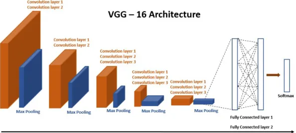
VGG-16 is a deep CNN model trained on ImageNet (Shallu and Mehra, R., 2018) (Sarkar, D., 2018) and can be used as transfer learning model. In this thesis work VGG-16 model was used for the primary data set classification. The network model consists of convolu-tion layers, pooling layers and fully connected layers. Figure 1-13 shows the network architecture of VGG-16.
Figure 1-13 Detailed architecture of a VGG-16 CNN model
Figure 1-13 explains the network architecture of VGG-16 by simplifying the divisions of convolution layers at the bottom. There are total 13 Convolution layers, two fully con-nected layers and one output layer. The default input feature shape for this network is 224 x 224. Chapter 4 and 5 present the implementation and results of CNN and transfer learning CNN models (ResNet-50 and VGG-16) used for current study.
The following chapter (2) of this thesis work present an overview of literature followed by methods (chapter 4) used for implementations. Chapter 3 briefly presents the rationale of this study approach. Final chapter (5) presents results and discussions on findings and observations of this thesis work.
2 Literature Survey
In this chapter a brief discussion on some of the previously used techniques to detect arrhythmia in ECG signals is presented. Since the focus of this thesis work is utilizing the neural networks for classification purposes therefore the literature survey is restricted more to machine learning and deep learning approaches. Sahoo et al. (2020) presents a comparative study of different machine learning techniques used for the interpretation of ECG and detection of arrhythmia present in it. Following sections in this chapter dis-cuss some of those techniques more in details. Moreover, a brief disdis-cussion on transfer learning via CNN is presented at the end of this chapter.
As discussed in the previous chapter, in most cases after the acquisition of ECG records, preprocessing is an important step to implement due to the noise present in the signal (Isin, A. and Ozdalili, S., 2017). Some of the important preprocessing steps involve dc (direct current voltage) noise removal from the ECG signal (Isin, A. and Ozdalili, S., 2017). This can be done by doing the mean subtraction method. Furthermore, moving average filters can be used to remove high frequency noise. High pass filters can be used for removing the low frequency noise. Isin and Ozdalili (2017) reported the use of band pass filtering for the removal of power line noise.
2.1 LSTM network model
In an attempt to classify arrhythmia using Long-short term memory (LSTM), (Yildirim, O. et al., 2019) proposed a new approach using convolutional auto-encoder (CAE). For this work, MIT-BIH ECG database (Moody, GB. and Mark, RG. 2001) was used. In this tech-nique compressed ECG signals were used for the classification purposes. This research study took place in two phases. Initially for data compression a deep CAE model was used and later the recognition was performed via a LSTM model. CAE model was pri-marily used to extract coded features.
(Yildirim, O. et al., 2019) reported the classification of 5 different types of beats including the normal beat NSR. The encoder part works on the original signal to get a feature vector of a smaller size as input for the LSTM while using up-sampling the decoder part reconstruct the original ECG signals. This research study produced an accuracy of over
99 %. Yildirim et al. (2019) reported a decrease of approximately 87 % in the training time by using the coded signal methods prior to LSTM model.
2.2 Adaptive Convolution neural network
(Kiranyaz, S. et al., 2015) presents a study for real time ECG classification based on individual person data using one dimensional CNN. This adaptive approach contains two primary steps of ECG classification i.e. extraction of features and final classification. For training purposes two different types of input data is used for each individual patient. Common features and individual patient’s data features. MIT-BIH database is used for the training purposes using this adaptive learning method. As explained by (Kiranyaz, S. et al., 2015), in a two dimensional CNN, the input for any
k
th neuron can be written as𝑥
= 𝑏 +
𝑐𝑜𝑛𝑣2𝐷 𝑤
, 𝑆
(4)Here
x
k is the input for the next layer in the network,b
k is the bias of thek
th neuron,w
k is the kernel weight for the current to the next layer andS
i is the output of thei
thneuron. And for one dimensional CNN (Kiranyaz, S. et al., 2015) rewrote Equation 4 as follows
𝑥
= 𝑏 +
𝑐𝑜𝑛𝑣1𝐷 𝑤
, 𝑆
(5)
The major differences between one and two dimensional CNNs are the vector data vs matrix data as well as scalar kernel size in one dimensional CNNs vs kernel windows in two dimensional CNNs. While using 44 records from MIT-BIH database, (Kiranyaz, S. et al., 2015) reported higher efficiency in speed and computation using this method.
2.3 Deep Convolution neural network and PTB
In another attempt to detect myocardial infarction (MI) disease from an ECG data strip, (Oh, S. et al. 2018) discusses a deep CNN based method. The ECG data used for this project work is obtained from Physikalisch-Technische Bundesanstalt (PTB) diagnostic ECG database (Goldberger AL. et al., 2003). 148 records were used from the normal
ECG data and 48 records were used with myocardial infarction. Table 2-1 (Oh, S. et al. 2018) shows some basic statistical information of the data used.
Table 2-1 Normal and Myocardial Infarction statistical data (Oh, S. et al. 2018)
Normal MI Minimum age 17 36 Maximum age 81 86 Average age 43.43 60.37 Number of males 39 110 Number of females 13 38
After preprocessing ECG data is segmented around the R peaks. Figure 2-1 (Oh, S. et al. 2018) shows the segmented ECG signals as Normal ECG and MI ECG.
Figure 2-1 Segmented Normal and Myocardial infarction ECG signals (Oh, S. et al. 2018)
An 11-layer network is used for the classification purposes using CNN. An efficiency of
2.4 Deep Convolution neural network and Categorical classification
In a study on deep CNN (Acharya, U. et al., 2017) presents the case of detecting 5 ECG beats classes. These classes are categorized as 5 super classes of 15 sub classes. Table 2-2 (Acharya, U. et al., 2017) shows the categorical division of these classes into 5 main classes of ECG beats.
Table 2-2 Categorical division of ECG beats into 5 classes (Acharya, U. et al., 2017)
N S V F Q
Normal Atrial premature Premature
ventric-ular contraction Fusion of ventric-ular and normal Paced Left bundle branch block Aberrant atrial
prem-ature Ventricular escape - Fusion of paced and normal Right bundle branch
block Nodal (junctional) premature - - Unclassifiable Atrial escape Supra-ventricular
premature - - - Nodal (junctional)
escape - - - -
Category N contains 90592, S contains 2781, V contains 7235, F contains 802 and Q contains 8039 beats to make a total size of 109449 beats, which were then used for the deep CNN. Similarly, to the previous case study discussed above, R peak detection is performed to segment the ECG beats. An overall accuracy of 89 % is achieved by de-ploying the CNN model as shown in Table 2-3 (Acharya, U. et al., 2017).
Table 2-3 CNN layers and kernel size information for each layer (Acharya, U. et al., 2017)
Layers Type No. of Neurons Kernel Size Stride
0–1 Convolution 258 × 5 3 1 1–2 Max-pooling 129 × 5 2 2 2–3 Convolution 126 × 10 4 1 3–4 Max-pooling 63 × 10 2 2 4–5 Convolution 60 × 20 4 1 5–6 Max-pooling 30 × 20 2 2 6–7 Fully-connected 30 – – 7–8 Fully-connected 20 – – 8–9 Fully-connected 5 – –
2.5 Transfer learning
(Isin, A. and Ozdalili, S., 2017) discusses the detection of cardiac arrhythmia via transfer learning. In this project an already trained deep learning model on a separate data was used to train and test ECG beats. MIT-BIH database is used, and three different beats namely normal, right bundle branch blocks and paced ECG beats were chosen for the training and validation purposes. After the acquisition of the data records, ECG data was preprocessed for noise removal. Pan-Tompkinds algorithm (Isin, A. and Ozdalili, S., 2017) was used to detect the QRS complex from the ECG recordings prior to network training. QRS detection was performed to extract the R-T segment from the ECG record-ings. Figure 2-2 (Isin, A. and Ozdalili, S., 2017) shows the graphical spread of three beats in training and testing data. Already trained AlexNet (Krizhevsky et al., 2012) model is used for the feature extraction and beat classification. Isin and Ozdalili (2017) reported an accuracy of 92 %. Figure 2-3 (Isin, A. and Ozdalili, S., 2017) shows the structure of the block view from data acquisition to classification steps.
Figure 2-2 Graphical spread of three different beats data on training and validation sets (Isin, A. and Ozdalili, S., 2017)
2.6 Other Machine learning methods
In various other studies including machine learning models, cardiac arrhythmia detection attempts are on record. Shadmand and Mashoufi (2016) report an accuracy of 97 % by employing temporal features from the ECG beats. S. Banerjee and M. Mitra (2014) re-ported an accuracy of approx. 98 % via cross wavelet transform for regular and irregular ECG beats. For efficient detection of R peak Hilbert transforms produced promising results as reported by (Benitez, D. et al., 2001). Rodríguez et al. (2015) reported an efficient technique of detecting QRS block by using Hilbert transform together with prin-ciple component analysis (PCA). Rodríguez et al. (2015) reported an accuracy of approx.
99 % for the detection of R peak in QRS block. By employing SVM model (Nguyen, M. et al., 2018) achieved an accuracy of 96 %.
2.7 Transfer learning efficiency parameters
In order to move towards the classification processes, different approaches were studied for the literature review in neural networks domain. Among various modern approaches using neural network, transfer learning stands out in terms of saving time and adaptabil-ity. Conventional machine learning techniques require training and testing data using one feature domain and distribution whereas in transfer learning a model trained on a related data can be used for another feature space (Zhang, L., 2020).
(Torrey, L. and Shavlik, J., 2009) suggests three parameters as the basis of improving performance using transfer learning. First is the Initial performance rate that can be reached in the target domain by using only the trained knowledge set. Second is how quickly the model learns the new tasks compared to the source task it has learned before used as a transfer model for transfer learning. Third is the eventual performance that can be acquired in the target space as compared to the eventual performance in the source space.
(Zhang, L., 2020) presents a case study of handwritten character recognition via transfer learning and suggests that transfer learning can save considerable amount of training time but slightly lowers the accuracy too. Zhang (2020) explains the schema of transfer learning from source to target feature space in Figure 2-4.
Figure 2-4 transfer learning from source to target feature space (Zhang, L., 2020)
2.8 ResNet work on MIT-BIH and PTB datasets
Deep CNN generally pose the problem of vanishing gradients and hence leads to a de-crease in accuracy as the model goes deeper because back propagation cannot update the parameters (Zhou, Y. et at., 2020). ResNet as a residual neural network offers the solution by means of feeding the future layers not only from the current layer of the neural network but also from the data that was used as input to this current layer. Figure 2.5 shows the main principle of ResNet. It can be noticed that activation function
f(x
)
is also fed the direct inputx
as identity as well as the previous layer’s throughput.To classify ECG beats, (Zhou, Y. et at., 2020) reported an accuracy of 99.2 % while working with MIT-BIH ECG dataset using Resnet with Bi - LSTM. Hammad et al. (2020) reported an accuracy of 98.8 % while using Resnet-Attention model on PTB database for human authentication via ECG records. Han and Shi (2019) acquired an accuracy of
95.49 % while working on PTB database using multi lead ResNet model.
2.9 VGG-16 and Breast cancer image model
Using 16-layer CNN model VGG-16 on breast cancer image data set (Shallu and Mehra, R., 2018) reported an accuracy of 92 %. Shallu and Mehra (2018) suggest that while comparing the accuracies of fully trained and fine-tuned networks, VGG-16 fine-tuned produced better results. During the fine-tuned training, some of the layers of pretrained network are changed according to current data set. However, most layers are kept frozen as they were trained on previous data sets.
3 Current State Analysis
Existing systems to classify ECG data are based on time series feature input to neural networks. Some of the methods include the usage of deep CNN for training and classifi-cation.
Generally, CNN performs better on two dimensional feature maps. Constant improve-ment of deep CNN based methods gives rise to new possibilities of learning and recog-nition. In contrast to conventional ECG methods, this research study presents the training of deep CNNs on two dimensional data. Originally the idea was introduced by (Jun, T et al. 2018). However present study adopts the training and classification using transfer learning with deep CNNs. Hence a novel idea of training and classifying two dimensional ECG data with transfer learning is presented in this thesis. ResNet-50 and VGG-16 CNN models are used to implement transfer learning.
4 Material and Methods
This thesis work is carried out as a research problem on ECG classification. The main stages of the project are data acquisition, preprocessing, neural network training and classification. Following sections in this chapter discuss these steps in more detail and present the in-depth view of implementations.
4.1 Database
For this project work MIT-BIH arrhythmia database (Goldberger et al. 2003) is used for the classification of ECG beats. Originally the dataset was downloaded and studied for the normal and abnormal beats. This dataset is accompanied by annotation files which help finding the marked beats as normal and or arrhythmia. In total 48 recordings from 47 patients are available from MIT-BIH dataset. An individual record is approximately half hour in length. Basic preprocessing such as band pass filtering was already per-formed on these records prior to their availability for research usage (Goldberger et al. 2003). Using Wave Form DataBase (WFDB) in Python programming environment ECG plots were studied and observed for beat markings. Figure 4-1 shows an ECG record using two limb leads acquired at a sampling frequency of 360Hz. Most of these ECG recordings were acquired from Limb Lead II and Lead VI using the Axial reference sys-tem (Goldberger et al. 2003), (Klabunde, R., 2017).
Figure 4-2 shows segment of an ECG signals acquired at 360 Hz using limb lead II and lead VI. For the implementation of this thesis work, Lead II signals have been used from the ECG strips as shows in Figure 4-3.
Figure 4-2 An extracted ECG signal from two leads
4.2 Preprocessing
As mentioned in the previous chapter, ECG signals are converted into images as the feature space of CNN. QRS complex detection was performed based on the location of the R peaks within the ECG strips. Annotation data was used to locate individual R peaks within these records as shown in Figure 4-4. Figure 4-5 shows markings of R peaks and the subsequent segmentation processes to separate beats individually as images.
Figure 4-4 R peak detection in an ECG strip and segmentation
Similarly, other ECG records were searched for individual R peaks and images were acquired and stored as image stack based on the type of beats i.e. normal and arrhyth-mia. Figure 4-5 shows the process of image stack acquisition from an ECG record.
Figure 4-5 Extraction of normal and arrhythmia ECG beats as images
Using the information provided in the annotation files, Arrhythmia types were selected for further processing in this thesis work. From a total of 48 records, 26 records were chosen to extract the images of ECG beats and 5 beat types were finally selected for the classification process. Figure 4-6 shows normal and 4 arrhythmia types i.e. premature ventricular contraction (PVC), left bundle branch block (LBBB), paced beats and right bundle branch block (RBBB) extracted as images from signals.
Table 4-1 shows the details of the segmented ECG images against 5 different beat types. For each arrhythmia type and normal beats, multiple patients’ records were used in order to get variability in the dataset.
Table 4-1 Summary of ECG records extraction as images
Arrhythmia PVC LBBB Normal Paced RBBB
No. of Beats 5000 5000 10000 5000 5000
# of patients records 8 5 12 7 9
4.3 Image processing and Encoding
CNNs are used for the classification of arrhythmia. Prior to network training and model execution, all images were reshaped to 224 x 224 with 3 channels for RGB values. Though input images are black and white but since the transfer learning models ResNet-50 and VGG-16 used in this thesis work are originally trained on RGB images from ImageNet data therefore ECG data images are used as RGB images with all three chan-nels having same values. These black and white RGB images can be loosely defined as RGB grey images. Images were then encoded based on individual representation of ar-rhythmia types as shows in Table 4-2.
Table 4-2 Categorical encoding of ECG beats
Arrhythmia PVC LBBB Normal Paced RBBB
Encoded as P L N P R
Using sklearn from keras libraries, label encoding was then performed to encode the arrhythmia codes as
0
and1
. Since there are five arrhythmia categories therefore, label encoding was carried out. Label encoding is performed to convert data values from non-numeric to non-numeric representation (Verkhivker, G. et al. 2019). Unlike decision trees and other statistical methods, machine learning and deep learning algorithms cannot work with categorial data and hence label encoding is performed prior to building classification models.4.4 Overfitting and Data augmentation
One of the advantages of using images as feature input for neural networks is the pos-sibility of enhancing dataset by data augmentation. Data augmentation is useful to over-come the problem of overfitting in machine learning models (Wang, J. and Perez, L., 2017), (Khandelwal, R. 2019). In general, larger learning data set makes a machine learning model more accurate on test data because network learns from more possibilities and avoid taking input from noise. This in turns leads to decrease in overfitting. Using data augmentation, data capacity is increased using the original training data by means of
datagen module in keras neural network library. For this project, data augmentation was performed using geometric operation on images such as zooming, rotation, translation and flipping as shown in Figure 4-7.
Figure 4-7 Result of data augmentation of an input image
4.5 Convolution neural network and classification
Deep CNNs are used for the training and classification of ECG data sets. Since image data input is used as features, therefore two dimensional convolutional methods are used in neural networks. Different primary classification groups were created to perform clas-sification on data sets (binary vs higher category sets) in varying combinations. There-fore, the Network architectures were changed and optimized according to input data set dimensions.
4.5.1 CNN models
For binary classification groups input data used as Normal vs PVC beats. A 9-layers deep CNN model was used for binary classification of image data set. ReLu activation function was used in the architecture of this neural network and input shape of 224 x 224
x 3 was selected. Figure 4-8 shows the architecture of the model used for the first clas-sification group. Keras neural network library in Python was selected for the implemen-tation of CNN models. Feature vectors were fed to the convolution layers followed by pooling layer where the padding features were kept same as input to the pooling layer. In order to avoid overfitting, dropout layers were used to drop some neurons in the net-work while training. Finally, Dense layers were used to reduce the size of the output vector gradually depending on the number of classes to be classified. In the case of two classes, unit value for dense layer was kept as 1 because it can predict either of the two possible outputs at a time.
Figure 4-9 shows the architecture of the model used for classification groups of 3 and 5 beat classes respectively. Due to higher variance in data, more dropout layers were in-troduced to avoid overfitting problem.
Figure 4-9 CNN model for 3 and 5 categories ECG data classification
4.5.2 Transfer learning
For transfer learning ECG beats in group of 2 and 5 were used with ResNet-50 and VGG-16 models. First group (Normal vs PVC) beats was trained on ResNet-50 and second group (Normal with PVC, LBBB, RBBB and Paced beats) was chosen for VGG-16 mod-els. Already trained ResNet-50 model contained layers including batch normalization to avoid overfitting, 2D convolution layers and max pooling. A 50 layers ResNet-50 network used for first group classification is presented in Figure 4-10.
The last layer of the ResNet model was set for training and all the preceding layers were frozen so that the weights trained on previous data can be used to train new features and classify classes of ECG beats.
Figure 4-10 ResNet-50 architecture for binary classification
VGG-16 Model already trained on ImageNet database, was used as a fully connected 16-layers CNN for 5 ECG beats classes classification. The network model consists of convolution layers, pooling layers and fully connected layers.
For the implementation of modified VGG-16 in current thesis study, last fully connected layers were removed and replaced by dense layers to classify ECG beats in 5 classes. This model wasn’t fine-tuned and thus all 13 layers preceding fully connected layers were frozen. Frozen layers weights were used in their original form and therefore did not get updated.
4.6 System description
For the implementation of this project following resources were used.
16 GB RAM
200 GB of storage
In order to perform prompt computations using CNN and to reduce the training time of models, Google Colab GPU was used with Python programming language. Colab short for colaboratory is a free tier google cloud service for Python programming in a browser view commonly used for deep learning implementations (Pessoa et al., 2018).
4.7 Neural network configuration
For implementing CNN based models, Python keras libraries were used for training and classification using neural network model layers. Few parameters from neural network implementations and their short explanations are given below.
Input shape: This is the shape of the data that is given to the neural network Batch size: This refers to the quantity of samples that are under processing
be-fore the neural network is updated
Epochs: This refers to a complete pass on the data being trained on neural net-works. For example, if an input of 1000 samples is given to the network then an epoch is completed when a certain number of times all 1000 samples are used once.
Loss: This refers to the error value that the model attempts to reduce during training. A decrease in loss value means model is converging for more accuracy. Some examples of loss calculation functions include (binary crossentropy and categorical crossentropy)
Optimizers: These refer to methods that alter the values of different model pa-rameters such as weights to reduce the loss value. Some examples include (RMSprop and Adam optimizers)
Batch Normalization: Just like in input data normalization at input layer, batch normalization normalizes the information at hidden layers to increase the learning capability of CNN.
5 Results
As mentioned in the previous chapter the original data was categorized in different groups prior to network model training and classification. In data preprocessing stage, Table 5-1 presents the summary of ECG beats extraction and it shows the details on the original dataset from MIT-BIH database. File number represents the original patient rec-ord as in MIT-BIH database.
Table 5-1 Statistical information of ECG data extraction from MIT-BIH arrhythmia database
Arrhythmia Group Normal Paced LBBB PVC RBBB
Extracted Labels n c l p r
Original Annotation Markings N / L V R
File number/Patients Records in MIT - BIH Directory 100 107 111 200 212 101 102 214 119 231 103 104 109 201 118 105 217 207 208 106 233 114 228 221 213 214 106 116
These extracted beats were then categorized as three main groups of Arrhythmia col-lections. First group consists of Normal and PVC beats. Second Group consists of rec-ords from Normal, PVC and Paced beats. While the last group consists of Normal, PVC, Paced, LBBB and RBBB beats. Table 5-2 - Table 5-4 show the description of classification data used for training.
Table 5-2 Normal and PVC ECG beats for classification
Arrhythmia Normal PVC Training Set Validation Set Test Set
Number of
Table 5-3 Normal, PVC and Paced beats for classification
Arrhythmia Normal Paced PVC Training
Set Validation Set Test Set Number of Samples 1200 600 600 2400 600 600
Table 5-4 Input data for 5 classes classification
Arrhythmia Normal PVC Paced LBBB RBBB Training Set Validation Set Test Set Number of Samples 1000 500 500 500 500 2000 1000 1000 5.1 Binary classification
Group 1 data was used for training and classification via CNN and ResNet-50 models in google Colab GPU powered environment. For CNN based training image dataset was resized to 224 x 224 for each image and pixel values were set in the range 0 and 255. Since Deep learning neural networks perform better with smaller values therefore indi-vidual data images were scaled in the range 0 and 1. In order to classify different groups image data labels were encoded using keras one hot encoder library. Table 5-5 shows the values of encoded data after one hot encoding.
Table 5-5 Binary classification label encoding (group 1)
Arrhythmia Normal PVC
Encoded Label 0 1
Image data set was then augmented and fed to the neural networks. In the case of Res-net-50 model the last layers were set as trainable and fully connected final layers were added. Since in Group 1 only two labels were used therefore binary crossentropy was used for loss and optimizer function was selected as RMSprop. In the case of CNN model observations were made repetitively and dropout layers were introduced in various ar-rangements until a constant accuracy was achieved with 3 dropout layers. A flatten layer was also introduced before the output layer to get the result as 1 node output. For Res-Net-50 two fully connected and two dropout layers were added on top of the frozen layers
of ResNet-50. Figure 5-1 shows the accuracy and loss graph of CNN model whereas Figure 5-2 shows the values for ResNet-50 model.
Figure 5-1 Accuracy and Loss values for binary classification of Normal and PVC beats
Figure 5-2 Binary classification of Normal and PVC beats using ResNet-50
Number of Epochs in both models were chosen at random and accuracy and loss curves were observed for fluctuations and convergence. Table 5-6 summarizes the resultant accuracies of both models.
Table 5-6 Accuracy of binary classification
Accuracy Measurement Training Set Validation Set Test Set CNN Accuracy ResNet-50 Accuracy Values 1460 360 360 83.1 % 83.5 %
5.2 Categorial classification
For Group 2 and 3, CNN models were trained on rescaled images between 0 and 1. Image dataset labels were encoded as shown in Table 5-7 for group 2 and in Table 5-8 for Group 3. Dropout layers were introduced to avoid overfitting and output layer was set to 3 and 5 nodes.
Table 5-7 3 classes ECG beats label encoding (group 2)
Arrhythmia Encoded Labels
Normal 1 0 0
Paced 0 1 0
PVC 0 0 1
Table 5-8 5 classes ECG beats label encoding (group 3)
Arrhythmia Encoded Labels
Normal 1 0 0 0 0
PVC 0 1 0 0 0
Paced 0 0 1 0 0
LBBB 0 0 0 1 0
RBBB 0 0 0 0 1
Number of epochs were set based on the first observation on accuracy and loss values. Since in group 2 and group 3, more than two categories are trained and classified there-fore categorical crossentropy was used for loss function and adam function was used as optimizer in keras model.
Figure 5-3 and Figure 5-4 show the resulting accuracy and loss values for group 2 and group 3 arrhythmia classifications. Table 5-9 shows the resulting accuracies of group 2 and group 3.
Figure 5-3 Accuracy and loss values for categorical classification of Normal, PVC and Paced ECG beats
Figure 5-4 Accuracy and loss values for categorical classification of Normal, PVC, LBBB, RBBB and Paced ECG beats
Table 5-9 Accuracies of 3 and 5 classes classification
Accuracy Measurement
Training Set
Validation Set Test Set Accuracy on 3
beats classification
Accuracy on 5 beats classification
5.3 Classification via VGG-16
Finally, the 5 beats classification is carried out with VGG-16 model to observe the accu-racy and efficiency via transfer learning on new data. For VGG-16 model the data set presented in Table 5-4 was used and the last fully connected layers of VGG-16 model were replaced by two dense layers for the classification of this data. Output layer con-tained 5 class output to classify from the test data set. VGG-16 was trained on 2500 ECG beat images and 1000 images were used for validation. Figure 5-5 shows the training accuracy and loss of the VGG-16 network whereas Figure 5-6 shows the confusion ma-trix on classification. The mama-trix on left side of confusion mama-trix shows the number of accurately recognized images in respective categories on the main diagonal while right side shows the same result in the form of heat map.
Figure 5-5 Classification of Normal, PVC, LBBB, RBBB and Paced ECG beats using VGG-16 CNN
5.4 Discussion
The Result chapter of this thesis work presents the observations and accuracies achieved on ECG dataset. Figure 5-1 to Figure 5-5 present accuracies achieved on im-age classification methods via three different CNN models. In all these models the overall minimum efficiency stayed higher than 83 %. Figure 5-1 and Figure 5-2 present the re-sults of two approaches i.e. 9 layers CNN and ResNet-50 respectively and their resulting performances on the same dataset. ResNet-50 model was improved in many iterations to achieve the similar efficiency as of multilayer CNN. Figure 5-3 and Figure 5-4 show that the regularization methods using dropout layers improved the results on categorial data as compare to binary label data. This also proves that higher number of categories and larger set of data helps the model learn better and yield improved classification re-sults.
In general Image classification research field has received a rather great impact from the methods of deep learning and CNNs. CNNs eliminated the requirement of feature ex-traction and therefore the focus can be now navigated more on self-learning models. Increasing amount of data as well as the varying complexity found in unrelated data sets are the major factors behind difficulty in early classification attempts via statistical meth-ods and traditional machine learning methmeth-ods. Deep CNNs used in this thesis work were studied for image set with very little significant information varying among its classes. Conventionally ECG signals are preprocessed and used in time series format for training and classification purposes. However, signals as one dimensional data may lose signif-icant information during preprocessing. In an ECG signal, noise removal filters may also compromise on important data information. Tradeoff are necessary to be made while working with signal data and specifically in deep learning-based classification. Since ECG beats do not vary much in their morphology therefore even with careful prepro-cessing, there exist chances of losing important peaks from data. Image extraction from ECG recordings on the other hand, tend to lose very little information. Hence, in terms of preprocessing the automatic feature extraction via deep learning models yield better results in classification processes (Jun, T. et al., 2018).
Implementation of deep CNN model via VGG-16 is the focus area of this study. The overall accuracy of VGG-16 is well above 99 %. VGG-16 resulted in smooth training and faster classification than a conventional neural network. Figure 5-6 shows that misclas-sification is significantly less for VGG-16 model and all 5 classes were classified within
99 % accuracy. ResNet-50 model also produced above 83 % efficiency on a binary label data but due to the complexity of the network, higher categorical data did not yield better results in this project study. Conventional deep learning models used for binary labels, 3 and 5 class ECG beat groups also produced promising results as shown in Table 5-6 and Table 5-9, however the accuracy of VGG-16 outperformed the results of other net-work models used. This clearly shows an improvement in classification methods by the introduction of transfer learning.
Since this thesis study was carried out on MIT-BIH Arrhythmia database therefore rele-vant literature material was studied and implementation methods were used as the basis for this thesis work. MIT-BIH and other online databases have a large amount of research literature available online and in research journals. Various methods including deep learning models were discussed in the literature survey chapter of this thesis. Kiranyaz et al. (2015) and Oh et al. (2018) reported accuracies higher than 95 % for one dimen-sional ECG data. Isin, A. and Ozdalili (2017) claimed 92 % accuracy while using transfer learning models. Tai et al. (2018) presented resulting accuracy of 99.05 % while using ECG data as images for deep learning CNN. This thesis study presents an attempt to combine some of the earlier techniques used on ECG data from MIT-BIH.
Implementing neural network models also poses difficult challenges in terms of under-standing network layers and their corresponding computations on tensor level. Problems such as over fitting and improper input shapes can result in weaker training of neurons and then lead to improper classification.
The choice of ResNet-50 and VGG-16 models was based on the higher efficiency and learning capability of these models. ResNet-50 proved to be working better for disap-pearing gradient issues since identity layer helps learning on deeper layers with previous true information on data. VGG-16 uses 3 x 3 convolution followed by a smaller pooling layer. The input feature size gets reduced in each layer and hence a simple, yet fast deep learning network is trained in less time than a conventional CNN and ResNet-50.
In first few classification attempts ResNet-50 did not produce promising results. Later with fine-tuning, ResNet-50 classification was improved where some of the frozen layers of ResNet-50 models were unlocked and set as trainable. Regularization largely im-proved the results by the introduction of dropout layers. One of the key challenges ap-peared during the implementation of transfer learning models was the incompatibly of
layers and output. Flatten layers in Keras neural network library helps reducing the di-mensions of the network layers to achieve the target size of the final layer.
This thesis work suggests a novel idea in terms of ECG data as images classified via transfer learning model VGG-16. As for future work more data will be tested, and results will be published in research journals. ResNet-50 model and its classification models will be studied in detail to match the results of VGG-16. Also, one dimensional ECG data comparative study will be carried out using multiple transfer learning models.
References
Abrol, A., Bhattarai, M., Fedorov, A., Du, Y., Plis, S. and Calhoun, V., 2020. Deep residual learning for neuroimaging: An application to predict progression to Alzheimer’s dis-ease. Journal of Neuroscience Methods, 339, p.108701.
Acharya, U., Oh, S., Hagiwara, Y., Tan, J., Adam, M., Gertych, A. and Tan, R., 2017. A deep convolutional neural network model to classify heartbeats. Computers in Biology and Medicine, 89, pp.389-396.
Aje, T., 2009. Cardiovascular disease: A global problem extending into the developing world. World Journal of Cardiology, 1(1), p.3.
Benitez, D., Gaydecki, P., Zaidi, A. and Fitzpatrick, A., 2001. The use of the Hilbert trans-form in ECG signal analysis. Computers in Biology and Medicine, 31(5), pp.399-406. Brownlee, J., 2019. A Tour Of Machine Learning Algorithms. [online] Machine Learning Mastery. Available at: https://machinelearningmastery.com/a-tour-of-machine-learning-algorithms/
Brownlee, J., 2016. Overfitting and Underfitting With Machine Learning Algorithms. [online] Machine Learning Mastery. Available at: <https://machinelearningmas-tery.com/overfitting-and-underfitting-with-machine-learning-algorithms/>
Brownlee, J., 2018. How to Develop 1D Convolutional Neural Network Models for Human Activity Recognition. [online] Machine Learning Mastery. Available at: <https://ma- chinelearningmastery.com/cnn-models-for-human-activity-recognition-time-series-clas-sification/> [Accessed 4 June 2020].
Ç. Sarvan and N. Özkurt, 2019, "ECG Beat Arrhythmia Classification by using 1-D CNN in case of Class Imbalance," 2019 Medical Technologies Congress (TIPTEKNO), Izmir, Turkey, pp. 1-4, doi: 10.1109/TIPTEKNO.2019.8895014.
Chang, K., Hsieh, P., Wu, M., Wang, Y., Chen, J., Tsai, F., Shih, E., Hwang, M. and Huang, T., 2020. Usefulness of Machine-Learning-Based Detection and Classification of Cardiac Arrhythmias with 12-Lead Electrocardiograms. Canadian Journal of Cardiology,.
Diker, A., Avci, D., Avci, E. and Gedikpinar, M., 2019. A new technique for ECG signal classification genetic algorithm Wavelet Kernel extreme learning machine. Optik, 180, pp.46-55.
E. Izci, M. A. Ozdemir, R. Sadighzadeh and A. Akan, 2018, "Arrhythmia Detection on ECG Signals by Using Empirical Mode Decomposition," 2018 Medical Technologies National Congress (TIPTEKNO), Magusa, pp. 1-4, doi: 10.1109/TIPTE-KNO.2018.8597094.
Gerlitz, Lars & Conrad, Olaf & Böhner, Jürgen. (2015). Large-scale atmospheric forcing and topographic modification of precipitation rates over High Asia - A neural-network-based approach. Earth System Dynamics. 6. 61-81. 10.5194/eds-6-61-2015.
Goldberger AL, Amaral LAN, Glass L, Hausdorff JM, Ivanov PCh, Mark RG, Mietus JE, Moody GB, Peng C-K, Stanley HE. PhysioBank, PhysioToolkit, and PhysioNet: Compo-nents of a New Research Resource for Complex Physiologic Signals (2003). Circulation. 101(23): e215-e220.
Gurney, K., 1997. Neural Networks – An Overview, An Introduction to Neural Networks. London: UCL Press. ISBN 0-203-45151-1
Halder, R., Chatterjee, R. and Mallick, P., 2019. Deep Learning based Smart Attendance Monitoring System. ResearchGate,.
Hammad, Mohamed & Pławiak, Paweł & Wang, Kuanquan & Acharya, U Rajendra, 2020, ResNet-Attention model for human authentication using ECG signals. Expert Systems. 10.1111/exsy.12547.
Han, Chuang & Shi, li, 2019, ML-ResNet: A novel network to detect and locate myocardial infarction using 12 leads ECG. Computer Methods and Programs in Biomedicine. 185. 105138. 10.1016/j.cmpb.2019.105138.
Hassan, M., 2018. VGG16 - Convolutional Network for Classification And Detection. [online] Neurohive.io. Available at: https://neurohive.io/en/popular-net-works/vgg16/https://www.cvphysiology.com/Arrhythmias/A013a
Isin, A. and Ozdalili, S., 2017. Cardiac arrhythmia detection using deep learning. Proce-dia Computer Science, 120, pp.268-275.
J. Huang, B. Chen, B. Yao and W. He, 2019, "ECG Arrhythmia Classification Using STFT-Based Spectrogram and Convolutional Neural Network," in IEEE Access, vol. 7, pp. 92871-92880, doi: 10.1109/ACCESS.2019.2928017.
Jaeger FJ. Cardiac arrhythmias. Cleveland Clinic. Retrieved 2010.
Joshi, A., 2019. How to Leverage Transfer Learning Using Pretrained CNN Models [Tu-torial] | Packt Hub. [online] Packt Hub. Available at: https://hub.packtpub.com/how-to-lev-erage-transfer-learning-using-pretrained-cnn-models-tutorial/
Jun, T., Nguyen, H., Kang, D., Kim, D. and Kim, Y., 2018. ECG arrhythmia classification using a 2-D convolutional neural network. School of Computing, Korea Advanced Insti-tute of Science and Technology, Daejeon, Republic of Korea,.
Khalaf, A., Owis, M. and Yassine, I., 2015. A novel technique for cardiac arrhythmia clas-sification using spectral correlation and support vector machines. Expert Systems with Applications, 42(21), pp.8361-8368.
Khandelwal, R., 2019. Deep Learning Using Transfer Learning -Python Code for ResNet-50 . [online] Medium. Available at: https://towardsdatascience.com/deep-learning-using-transfer-learning-python-code-for-ResNet-50 -8acdfb3a2d38
Kiranyaz, Serkan & Ince, Turker & Gabbouj, Moncef , 2015, Real-Time Patient-Specific ECG Classification by 1D Convolutional Neural Networks. IEEE transactions on bio-med-ical engineering. 63. 10.1109/TBME.2015.2468589.
Klabunde, R., 2017. Electrocardiogram Standard Limb Leads (Bipolar), Cardiovascular Physiology Concepts. [online] Cvphysiology.com. Available at:
Kononenko, I., 2001. Machine learning for medical diagnosis: history, state of the art and perspective. Artificial Intelligence in Medicine, 23(1), pp.89-109.
Krizhevsky, A., Sutskever, I., Hinton, G. E., 2012. Imagenet classification with deep con-volutional neural networks. Advances in Neural Information Processing Systems, 1097– 1105
Levick, J., 1991. Chapter 4 - Electrocardiography, An Introduction to Cardiovascular Physiology. London: Butterworth-Heinemann, pp.45-54.
Li, Y. and Cui, W., 2019. Identifying the mislabeled training samples of ECG signals using machine learning. Biomedical Signal Processing and Control, 47, pp.168-176.
Liu, B., Liu, J., Wang, G., Huang, K., Li, F., Zheng, Y., Luo, Y. and Zhou, F., 2015. A novel electrocardiogram parameterization algorithm and its application in myocardial in-farction detection. Computers in Biology and Medicine, 61, pp.178-184.
Liu, D., 2017. A Practical Guide to Relu. [online] Medium. Available at: https://me-dium.com/@danqing/a-practical-guide-to-relu-b83ca804f1f7
Mathews, S., Kambhamettu, C. and Barner, K., 2018. A novel application of deep learning for single-lead ECG classification. Computers in Biology and Medicine, 99, pp.53-62. Mebsout, I., 2020. Convolutional Neural Networks’ Mathematics. [online] Medium. Avail-able at: https://medium.com/swlh/convolutional-neural-networks-mathematics-1beb3e6447c0
Moody GB, Mark RG. The impact of the MIT-BIH Arrhythmia Database. IEEE Eng in Med and Biol 20(3):45-50 (May-June 2001). (PMID: 11446209)
Moore, K.L. , Dalley, A.F. , Agur, A.R. 2013 Clinically oriented anatomy Wolters Kluwel Health/Lippincott, Williams & Wilkins
Nguyen, M., Shahzad, A., Nguyen, B. and Kim, K., 2018. Diagnosis of shockable rhythms for automated external defibrillators using a reliable support vector machine classifier. Bi-omedical Signal Processing and Control, 44, pp.258-269.
Oh, S., Ng, E., Tan, R. and Acharya, U., 2018. Automated diagnosis of arrhythmia using combination of CNN and LSTM techniques with variable length heart beats. Computers in Biology and Medicine, 102, pp.278-287.
Pessoa, T., Medeiros, R., Nepomuceno, T., Bian, G., Albuquerque, V.H.C. and Filho, P.P., (2018). Performance Analysis of Google Colaboratory as a Tool for Accelerating Deep Learning Applications. IEEE Access. PP. 1-1. 10.1109/ACCESS.2018.2874767. Phukpattaranont, P., 2015. QRS detection algorithm based on the quadratic filter. Expert Systems with Applications, 42(11), pp.4867-4877.
Rahhal, M., Bazi, Y., AlHichri, H., Alajlan, N., Melgani, F. and Yager, R., 2016. Deep learning approach for active classification of electrocardiogram signals. Information Sci-ences, 345, pp.340-354.