The effect of spatial RNNs on neural network feature maps

TECHNISCHE UNIVERSITÄT MÜNCHEN

Master Thesis in Computer Vision

The effect of spatial RNNs on neural

network feature maps

DEPARTMENT OF INFORMATICS

Master Thesis in Computer Vision

The effect of spatial RNNs on neural

network feature maps

Author: Oriol Vila Clarà

Supervisor: Prof. Dr. Laura Leal-Taixe Advisor: Tim Meinhardt

Abstract

Computer vision applications and specifically image classification tasks usually rely on convolutional layers in order to extract information form input images and process the feature maps. In this thesis we experiment and study the effects of applying sequence recurrent neural networks (RNN) to spatial feature maps. A new approach introduced by ReNet, Inside-Outside Network and PoseNet LSTM where sequence RNN are used to process 2D feature maps and improve the performance of the network. In this thesis we evaluate different toy models in the MNIST and CIFAR10 datasets to observe which are the best practices when applying the RNN and discover in which way can they improve the performance.

Abstract iii

1 Introduction 1

1.1 Statment of purpose . . . 1

1.2 Requirements and specifications . . . 1

1.2.1 Project requirements . . . 1

1.2.2 Specifications . . . 2

2 Artificial neural networks 3 2.1 Feed-forward Neural Networks . . . 4

2.1.1 Fully Connected Layers . . . 4

2.1.2 Convolutional Layers . . . 4

2.2 Recurrent Neural Networks . . . 5

2.2.1 Long Short-Term Memory . . . 6

2.2.2 Gated recurrent unit . . . 6

2.3 Regularization for Neural Networks . . . 7

2.3.1 Dropout . . . 7

2.3.2 Batch normalization . . . 8

2.3.3 Weight Decay . . . 8

2.4 Supervised training of Neural Networks . . . 8

2.4.1 Back-propagation algorithm . . . 8

2.4.2 Mini-Batch Gradient Descent (SGD) . . . 9

2.4.3 Model evaluation . . . 9

3 State of the art 10 4 Experimental results 13 4.1 Methodology . . . 13

4.2 Model selection . . . 13

4.2.1 Two Multilayer Perceptron (2MLP) . . . 14

4.2.2 One Multilayer Perceptron (1MLP) . . . 14

Contents

4.3 Setup environment . . . 16

4.3.1 Training dataset . . . 16

4.3.2 Momentum and weight decay . . . 16

4.3.3 RNN input size . . . 16

4.3.4 RNN input shape . . . 17

4.4 Accuracy . . . 18

4.4.1 Model depth . . . 19

4.4.2 Hidden size . . . 20

4.5 Learning rate robustness . . . 20

4.5.1 Hidden size . . . 22

4.5.2 Full network range . . . 25

4.5.3 Truncated network range . . . 27

4.5.4 Hypothesis . . . 29

4.6 Other experiments . . . 30

4.6.1 Double learning rate . . . 30

4.6.2 Full LSTM network . . . 30

4.6.3 Full sequence output . . . 31

4.6.4 Other architectures . . . 32

5 Conclusions 33 5.1 Accuracy . . . 33

5.2 Learning rate robustness . . . 34

5.3 Future work . . . 34

List of Figures 35

List of Tables 36

Recurrent neural architectures, alongside all its other variations like LSTM and GRU units, have shown very promising results when working with sequential data; tasks such as language modeling, machine translation and time related applications are the most common examples. Despite that, recent work has shown that it is also possible to apply sequence RNN directly to multidimensional feature maps using a four directional sweeping mechanism which has been proven to be a very effective way of processing multidimensional inputs without using more complex multidimensional RNN architectures. After reviewing these works and specially after seeing the potential that was shown on the PoseNet LSTM paper [20], we decided to further explore these particular networks, study its performance, implications and how applying RNNs to neural network feature maps can improve their performance.

1.1 Statment of purpose

The objective of this master thesis is to further explore the benefits of adding spatial RNNs into neural networks and study its effects, specifically neural networks related to computer vision applications such as pose regression and image classification.

This work is centred on the observations of what happens when RNNs are applied into different network architectures and configurations and how the performance and behaviour changes. Different recurrent units such as RNNs, LSTMs and GRUs are evaluated. At the same time, parameters like the number of hidden neurons, the learning rate and the number of layers are also analyzed.

1.2 Requirements and specifications

1.2.1 Project requirements

1. Revise the pytorch version of PosNet [13] and implement the LSTM regression heads based on the F. Walch thesis [20] in order to reproduce the paper results. 2. Develop a Pytorch working environment in order to evaluate the different model

1 Introduction

3. Analyze and evaluate the performance of the selected networks with and without the addition of spatial RNN in the architecture.

1.2.2 Specifications

1. The project is developed in Pytorch 0.4.

2. Visdom and TensorboardX are used for the visualization of the gradient distribu-tion, the weight histograms and the training loss-accuracy.

3. The software implements multiple seed averaging, data sub-sampling and inde-pendent learning rate for different modules.

4. More than twenty different models that can be configured from a wide range of parameters are implemented.

This chapter presents the theoretical background about the artificial neural networks which this project is based on. Section 2.1 presents the fundamentals of these networks that are described along the most basic structures that can be build: the feed forward Neural Networks. In 2.2 section, recurrent neural networks (RNNs) are explained alongside the most relevant variations like LSTM and GRU which are the main research line of this thesis.

Artificial Neural Networks are a very popular machine learning architecture that is based on artificial neurons. These neurons behave in a similar way as the brain cells by receiving one or more inputs and producing an output response. Each input is separately weighted and the sum goes through a non-linearity known as the activation function. Mathematically, a single artificial neuron with k input values represents a non-linear function g : RK → R, parametrized by a weight vector w, a biasb, and a non-linear activationσ. Figure 2.1 shows an illustration of this structure.

Figure 2.1: Illustration of an artificial neuron with its mathematical formula. Image extracted from [19].

By combining multiple of this units, it is possible to create a neural network which defines a function that maps input data to output values. Depending on the network application, these outputs are used as regression or as class scores for classification.

2 Artificial neural networks

2.1 Feed-forward Neural Networks

A feed-forward neural network is the result of arranging the artificial neurons into layers. Each neuron of the layerl feeds its output only into the neurons of the next layer l+1 so that the feed-forward property is constituted as the information only goes forward. There are not any cycles or loops like the recurrent neural networks. The number of neurons in each layer determines the width while the number of layers determines the depth of the network. Each neuron from one layer has direct connections to the neurons of the subsequent layer.

2.1.1 Fully Connected Layers

A fully connected layer is the most simple element we can find in a neural Network where each input from the layer below is connected to every single neuron of the next layer.

2.1.2 Convolutional Layers

In convolutional layers every neuron is only connected to an small region of the multidimensional input in which the weights of the different patches are shared. This local connectivity decreases the total number of parameters and makes these kind of layers very suitable for image processing tasks.

The same operation can also be seen as a convolution of the input data with a set of filters or kernels which generate a feature map. The layers parameters are the learnable filters with a fixed width and height, extending through the full depth of the input volume. The area of these filters is also called the receptive field or kernel size. Some other parameters such as stride, padding and the number of filters define the output shape and how the convolutions are computed. An example of a convolutional layer applied to an input image is shown on figure 2.2.

Convolution layers are usually followed by a pooling operation that reduces the area of the feature maps by a down-sampling. It can be done either using a max operation between neighbours (max Pooling) or the average of them (Average pooling). These operations manage to reduce the number of parameters of the following layers and make the feature maps more robust to image shifts and variations.

Figure 2.2: Illustration of how a convolution layer is applied to an input image. The filterwextends to the full input depth but with a fixed width and height. The output depth is determined by the number of filters. Image extracted from [6].

2.2 Recurrent Neural Networks

The networks presented so far produce a deterministic output for each input they receive, independent from previous inputs or outputs. Recurrent neural networks, in the other hand, are a form of neural networks adapted to work with sequential data which take decisions based on current and previous inputs. Figure 2.3 illustrates this structural difference.

Figure 2.3: Illustration of a RNN compared to a feed-forward network. Figure extracted from [7].

2 Artificial neural networks

There are usually different kind of recurrent units based on how the current and last inputs are combined. The default version of recurrent unit, also called vainilla RNN, is the one in which the output is treated like another input.

2.2.1 Long Short-Term Memory

LSTMs were proposed in 1997 by Sepp Hochreiter and Jürgen Schmidhuber [10] and were refined and improved in the following years [8]. They are a special kind of RNN capable of learning long-term dependencies thanks to a cell state which retains the information of previous inputs. Moreover, it also has the ability to remove or add information with a gating mechanism. Figure 2.4 shows an LSTM diagram with its mathematical equations.

Figure 2.4: Diagram of the LSTM unit with its mathematical equations. Figure extracted from [15].

2.2.2 Gated recurrent unit

Introduced in 2014 by Kyunghyun Cho et al [5], GRUs are an improved version of standard recurrent neural networks. The architecture is based on a gating mechanism constituted by an update and reset gate which decide what information should be passed to the output. Therefore, they can be trained to keep information from long ago, without washing it through time or remove information which is irrelevant to the prediction. The performance of GRUs is very similar to LSTMs but they offer a more simple structure. In some cases they have been shown to provide with better perfor-mance on smaller datasets. Figure 2.5 shows a GRU diagram with its mathematical equations.

Figure 2.5: Diagram of the GRU unit with its mathematical equations. Figure extracted from [15].

2.3 Regularization for Neural Networks

One of the challenges we face when training Neural Networks is the over-fitting problem. We want the model to generalize on the data assuring that the network will perform well not only on training data but also on new inputs as well. The training data contains information about the regularities in the mapping from input to output but it also contains sampling error. Therefore, when we fit the model, it cannot tell which regularities are real and which are caused by the sampling error; leading to problems when generalizing over new data.

In order to solve this problem, we could try to gather more data, set the optimal capacity of the network for the existing data or add regularization techniques which modify the network to reduce its generalization error. Multiple solutions already exist to cope with this problem such as Dropout, Batch normalization and Weight Decay.

2.3.1 Dropout

Dropout[17] is a way to regularize a neural network. During the training, it may happen that neurons of a particular layer become influenced only by the output of a particular neuron in the previous layer. In that case, the neural network would overfit. Dropout prevents overfitting and regularizes by randomly cutting the connections (also known as dropping the connection) between neurons in successive layers during the training phase.

2 Artificial neural networks

2.3.2 Batch normalization

Batch normalization [11] is a technique for improving the performance and stability of neural networks. The core idea is to normalize the inputs of each layer in such a way that they have a mean output activation of zero and a standard deviation of one; the same procedure as it is usually done in the input layer. By using batch normalization we get multiple benefits like training faster, being able to use higher learning rates, allowing more activation functions, etc. It also reduces over-fitting because it has a slight regularization effect. Similar to dropout, it adds some noise to each hidden layer activation and helps to generalize the data.

2.3.3 Weight Decay

When training neural networks it is common to use weight decay. In this method the weights are multiplied by a factor slightly less than 1 after each update preventing them from growing too large. L2 regularization is perhaps the most common form of regularization and it can be implemented by penalizing the squared magnitude of all parameters directly in the objective. Thus, for every weightwin the network we add the term 1₂λw2to the objective, whereλis the regularization strength.

2.4 Supervised training of Neural Networks

As stated in the beginning of this chapter, neural networks are able to calculate an outputy from an inputx given the network parameters. In supervised learning for neural networks, the goal is to learn the functiony = f(x)that maps the input-output pairs by approximating it with a neural network. This function is unknown and it can be learned trough a set of labeled data which contains input examples alongside its correct outputs.

At the start of the training, the weights and biases that conform the neural network are initialized to random values and we feed the network with the training data. The outputs are then compared with the corresponding labels and the training error or loss is calculated. By adjusting the network parameters to minimize the loss, we can indirectly try to approximate the target function with our neural network.

2.4.1 Back-propagation algorithm

The most common way of updating the network parameters while minimizing the loss is through the back-propagation algorithm. This optimizing method is based on the gradient decent technique to adjust the weight of neurons by calculating the gradient of

the loss function. The chain rule is used to iteratively compute gradients for each layer. For recurrent neural networks, a similar technique is used: it is called backpropagation through time (BPTT).

2.4.2 Mini-Batch Gradient Descent (SGD)

Rather than evaluating a cost function over the entire training set (as in Standard Gradient Descent), SGD uses a subset of the training data (a minibatch) that is randomly selected from the training dataset. The weights are updated at every minibatch thus having a higher update frequency which allows a more robust convergence, avoiding local minima. Partially thanks to the regularization effect due to the randomness and noise introduced in the mini-batch sampling. With the batching method we are not required to have all training data in memory and we can use highly optimized libraries that make computing the gradient on a mini-batch very efficient.

The SGD optimization algorithm can be further improved by using the momentum method [16]. Stochastic gradient descent with momentum remembers the update∆wat each iteration, and determines the next update as a linear combination of the gradient and the previous update. This method can further help the network to hop out of local minima and to converge faster.

2.4.3 Model evaluation

When training neural networks we also need to adjust some hyper-parameters and evaluate how the model is performing on unseen data. Therefore, it is very common to split the total dataset in three different folds: training dataset, validation dataset and test dataset. The training dataset is used to fit the model into the data while the validation dataset provides an unbiased evaluation of the model. It allows us to tune some hyper-parameters like the early stopping mechanism to decide when to end the training phase. Finally the test dataset gives us the final evaluation of the model and verifies if the objective has been achieved.

3 State of the art

This chapter presents the main research line of this thesis which is the study of the recurrent neural networks when used for spatial processing of feature maps. In the following sections, the latest works and literature about the same topics are reviewed in order to give some context to the thesis objectives and experiments.

Recurrent architectures have been successfully applied to solve machine learning problems for more than 25 years. They are more often used in temporal sequences and language modeling than they are for processing multidimensional feature maps, as these examples have a natural sequence form. But in the year 2007, Alex Graves introduced the MDRNNs [9] which were directly applied on multidimensional feature maps. Since then, they were also widely adopted in computer vision tasks in the following years like handwriting classification [9], texture segmentation [3] and scene labelling [4]. This was the first time that RNNs were directly used to an spatial input so as to process a multidimensional feature maps.

Figure 3.1: ReNet layer ap-plied directly to the input image. Image extracted from [18].

MDRNNs replace every single recurrent connection from standard RNNs withdconnections, wheredis the number of spatio-temporal data dimensions. This makes it possible to apply this recurrent architecture to multidimensional fea-ture maps. MDRNN were the first reccurrent unit used for computer vision tasks that was directly applied to feature maps.

It was not until 2015 that Visin et al. [18] proposed the ReNet architecture in which instead of using multi-dimensional RNNs they used the standard sequence one-dimensional LSTM to process multione-dimensional inputs by sweeping the image vertically and horizontally in both directions. This process is shown in figure 3.1. The first horizontal sweep is directly applied to the input image and its output processed by the second layer from the vertical direction using the full sequence length. By doing this procedure multiple times and with a fully connected layer at the end, the ReNet Network is able to extract the features

of the image and make the classification. ReNet performed quite well on different datasets like CIFAR10, MNIST and SVHN, showing that spatial RNN were a viable alternative to the convolutional layers for image classification.

After ReNet, more architectures followed the same approach. Sean Bell et al. pro-posed the Inside-Outside network [1] which was also using sequence RNN to process feature maps. This time, instead of using them as the core network structure, they were used at a specific location after the last convolutional layer to process high level features and get spatial information. In this implementation they were also using the full sequence output concatenating the output of the four possible directions at each time step simultaneously.

F. Walch et al. used the same basic principle of the four directional LSTM to improve the accuracy of the PoseNet Network [20]. They added a four directional LSTM layer after one of the last fully connected layers. The input was artificially reshaped in a 2D shape an then swept by the LSTM to process the feature map. Doing so, there was an impressive accuracy improvement of the network that highlighted the potential of spatial RNNs. The full architecture of the PoseNet LSTM network is shown in the figure 3.2.

Figure 3.2: Architecture of the PoseNet LSTM Network. Image extracted from [20]. This last PoseNet LSTM paper inspired this thesis to explore if this idea could be generalized to other network architectures and applications. Moreover, another focus of the thesis was getting some insights on how the LSTM was working

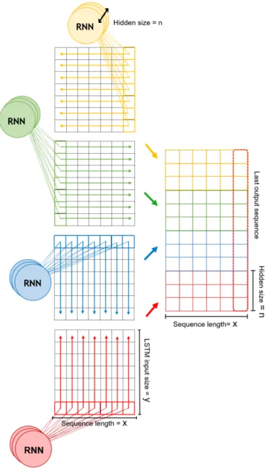
Figure 3.3 shows in more detail the procedure of applying a four directional RNN to a feature map. This is the same method used both in PoseNet LSTM [20] and the models proposed in this thesis.

3 State of the art

Figure 3.3: Ilustration on how the RNN units are applied to the 2D feature maps. The rows and columns of the feature map are used as an input by the four recurrent units that sweep the image into the four possible directions simultaneously. At each time step, a new input is consumed and the the hidden states of each unit are concatenated into a single vector. We get a 2-dimensional output after the whole input has been processed.

After implementing the PoseNet LSTM described in [20] and checking that the addition of LSTMs was showing a better performance on the Cambridge Landmarks Dataset, we decided to switch to more simple models and datasets in order to see if this behaviour was still replicable. We then proceeded with different experiments to get a better idea on how the RNNs were working.

4.1 Methodology

To conduct all the experiments explained below, we decided to use the stochastic gradient descent algorithm for the optimization process. The loss is calculated as the average cross entropy of all the samples in the mini batch. We obtained the performance results of the different models by using always a test dataset consisting of 10k images for the best training model which was obtained as the one that achieved the best classification accuracy in the validation dataset, also a sized 10k images.

The validation was performed at the end of each training epoch until the end of the training where there was more than 100 epochs in which the validation accuracy did not improve. The accuracy and loss results were calculated as the average of three different seeds that were using the same shuffled and re-sampled training database. All the datasets were normalized, the weights randomly initialized and for the recurrent modules, the hidden states were reset to random distributions after each sequence was completed.

4.2 Model selection

The first step to get started with this project was to decide the architecture of the models to be tested. We wanted to see in which way the RNN could improve the performance on different network architectures and configurations so we selected three different models. They were different between each other but they maintained some similarities to the networks used in the previous work that we took as a reference.

For each model proposed we always test two versions: The default fully connected version and the RNN version in which one of the fully connected layers is replaced for

4 Experimental results

a four directional RNN. In this way we can see how the RNNs change the behaviour of the network, which is the main objective of this thesis. In both versions the number of parameters is always the same in order to make a fair comparison. We proposed three different models which are going to be explained in the following sections.

4.2.1 Two Multilayer Perceptron (2MLP)

This model (illustrated in figure 4.1) consists of a multi-layer perceptron with two hidden layers or more (2 hidden layers are the default if not specified otherwise). As usual, the layer before the last fully connected is replaced by a four directional RNN in the recurrent version. We also have an artificial reshaping on the last layers with the same procedure as in [20]. The most important characteristic of this model is that we can easily control different parameters like the hidden size, RNN input size and shape while maintaining the total number of parameters by changing the size of the first fully connected layers.

(a) Fully connected version (b) RNN version

Figure 4.1: Ilustration of the 2MLP model. Images based on [12]

4.2.2 One Multilayer Perceptron (1MLP)

The second model, called 1MLP (illustrated in figure 4.2) is also a multi-layer perceptron with just one hidden layer in the fully connected version that is replaced by the four directional RNN in the RNN version. But even though it looks really similar to the 2MLP, the basic principle is completely different, as the RNNs are directly applied to the input image instead of higher level features. This is also the same model used in [2] which is used on numerous benchmarking experiments. Thanks to this paper we got some guidelines on what to expect when evaluating this model.

(a) Fully connected version (b) RNN version

Figure 4.2: Illustration of the 1MLP model. Images based on [12]

4.2.3 Convolutional Neural Network (CNN)

This model has a very similar architecture to LeNet [14]. It is composed by two convolutional layers with max pooling followed by three fully connected layers, one of which is replaced by a 4 directional RNN in the recurrent version. The interesting characteristic of this model is that the RNNs are applied to high-level features that come from the convolutional part and the first fully connected layer. This is the experimental model closer to PoseNet LSTM architecture [20]. In this case the network is very suited for the MNIST dataset, achieving much better accuracy that the other two models. The two versions of the model can be seen in figures 4.3 and 4.4.

4 Experimental results

Figure 4.4: Illustration of the model CNN RNN version. Images based on [12].

4.3 Setup environment

Before starting with the evaluation of the different models, several hyper-parameters needed to be fixed because there were not relevant to the research or because they were a critical part of the design. In some cases, we conducted some preliminary experiments to get the optimal parameters and they were set as default for the following experiments.

4.3.1 Training dataset

The nature of our experiments was to observe small changes between different network architectures and RNN versions in a controlled environment. That is why we needed a simple dataset where the toy models could achieve good performance and it was easy to control some side effects like over-fitting. The training size was set to 500 as it was faster to train and the variance between the different models and versions was higher thus making the performance easier to evaluate.

4.3.2 Momentum and weight decay

Momentum and weight decay were two other important parameters to be decided. After some experiment they were set to 0 as they did not seem to affect the results. By doing so we also had less parameters to take into consideration when studying the effect of the RNN for feature map processing.

4.3.3 RNN input size

The four directional RNN is directly applied to feature maps that can have different sizes and shapes. In all the cases when the previous layer is fully connected, it is

possible to define the feature map size by adjusting the number of neurons. Therefore the four directional RNN input can be defined. PoseNet LSTM [20] used input sizes around 32x32 and when the RNN is directly applied to the input image like in [2], the input needed to be set either to 28x28 or 32x32 depending on the dataset. Because of this, we decided to set the input sizes around 32x32 whenever was possible. We also conducted an experiment with a 2MLP model with three hidden layers on which we tested different input sizes and we proved that a size around 32x32 seemed reasonable. Looking at the results displayed on the table 4.1 we can see that different input sizes have similar performances.

Input size

First layer size Second layer size Reshaping Accuracy

1934 256 16x16 88.75±0.15

1524 529 23x23 88.86±0.19

1094 1024 32x32 88.74±0.16

784 1764 42x42 88.63±0.19

Table 4.1: Accuracy results on the 2MLP model using different input sizes.

4.3.4 RNN input shape

In some cases the feature maps to be processed by the RNN were one-dimensional (for example the output of fully connected layers). In order to get the best performance, the input needed to be artificially reshaped to a 2D form. Therefore, the form of this reshape was a new hyper-parameter to be defined. In [20] they used both square and rectangular shapes, but at the end, the best configuration was achieved by a 32x64 shape.

We also conducted some experiments with different input shapes, and it was shown that a rectangular shape seemed to be the best configuration. One interesting side-note of this experiment was that the optimum learning rate slightly decreased when using more rectangular shapes which can be the reason of this performance difference. But in the end, as the differences where not significant and because the input shape of the 1MLP model could not be altered, we decided to fix our input shape to a square whenever ti was possible. The results of this experiment are shown on the table 4.2

4 Experimental results

Input shape

Shape Reshaping Accuracy Square 36x36 88.38±0.28 Rectangular 2:1 54x24 88.75±0.02 Rectangular 4:1 72x18 88.59±0.29 Rectangular 20:1 162x8 88.67±0.22 Rectangular 80:1 324x4 88.88±0.15

Table 4.2: Accuracy results on the 2MLP model using different input shapes.

4.4 Accuracy

The accuracy improvement was one of the expected results by adding RNNs into the networks so we were expecting the RNN versions to perform better than the fully connected counterparts. Despite that it was not always the case, and the results shown in tables 4.3, 4.4 and 4.5 were more dependent to the network architecture than we thought.

MNIST Accuracy

Model Name LSTM FC Accuracy difference 2MLP 88.38±0.28 88.48±0.12 -0.10pp 1MLP 89.65±0.31 87.13±0.34 +2.52pp CNN 94.80±0.33 93.75±0.35 +1.05pp

Table 4.3: Accuracy of the 2MLP, 1MLP and CNN models on the MNIST database using 500 training samples. RNNs are able to improve the accuracy of 1MLP and CNN models but not on the 2MLP.

Diferent training size MNIST accuracy

Model Name 500 5k 40k

2MLP -0.1pp -0.3pp -0.15pp 1MLP +2.52pp +2.93pp +1.49pp CNN +0.8pp +0.16pp +0.01pp

Table 4.4: Accuracy of the 2MLP, 1MLP and CNN models on the MNIST dataset using different training sizes. The 2MLP model is the only one that does not benefit from the RNNs.

CIFAR10 Accuracy

Model Name LSTM FC Accuracy difference 2MLP 42.88±0.08 44.48±0.18 -1.6pp 1MLP 42.68±0.04 41.01±0.4 +1.64pp

CNN 53.23±0.27 52.39±0.35 +0.11pp

Table 4.5: Accuracy of the 2MLP, 1MLP and CNN models on the CIFAR10 dataset using 5k training samples. As seen in the MNIST dataset, the 2MLP is the only model where RNNs are not improving the results.

while the other models seems to benefit slightly from the RNNs. These observations are happening both in MNIST and CIFAR10 datasets and also when using different training sizes. As the training size grows larger, the gap between the two versions is also closer, probably because the accuracy is already really high and closer to the limit. This behaviour can resemble some kind of regularization effect introduced by the RNNs although further tests and experiments are required before drawing any conclusions.

4.4.1 Model depth

One of the first hypothesis that can be drawn, is that it seems that RNN benefits from either structured spatial inputs (when it is directly applied to the image like in 1MLP) or high level features after several layers. This could be the reason that CNN performs better with RNNs than the 2MLP model. To prove this hypothesis we also tried to increase the depth of the 2MLP model by adding more hidden layers. The results are displayed in the table 4.6.

Model depth

Model LSTM FC Accuracy difference

2MLP 88.35±0.13 88.72±0.21 -0.38pp 3MLP 88.85±0.28 88.58±0.59 +0.27pp 4MLP 88.56±0.15 88.11±0.28 +0.45pp

Table 4.6: Accuracy of the model 2MLP with different layers depth. Notice that the deeper the model is, the better the accuracy difference between the RNN version and the fully connected.

4 Experimental results

4.4.2 Hidden size

The number of neurons in the RNN, called hidden size, is an important hyper-parameter when defining RNN networks. In order to study how this parameter is linked to the network performance, we decided to make some testing with the different models and see which hidden sizes offered better accuracy.

(a) 2MLP model (b) 1MLP model (c) CNN model

Figure 4.5: Hidden size accuracy. Low hidden sizes offer better accuracy overall. Overall, all the models have a similar behaviour when adjusting the hidden size. As shown by the figure 4.5, smaller hidden sizes offer better accuracy in all of the three models we tested. Usually the hidden size has to be larger than 10 units but less than 256 because outside this range there is a big accuracy drop. The same behaviour was observed in Benchmarking of LSTM Networks [2] where small hidden sizes were performing better.

4.5 Learning rate robustness

One of the first observations we made when testing the different models was the accuracy was strongly dependant to the learning rate. Each model had its optimum learning rate which is usually higher for the RNN versions. Figure 4.6 and 4.7 shows the accuracy for both versions of the 2MLP model using different learning rates.

Figure 4.6: Learning rate robustness of the LSTM versions. The networks are able to work in a wide range of learning rates.

Figure 4.7: Learning rate robustness of the fully connected versions. After a certain learning rate threshold the networks stop working.

RNN versions do not only have a higher optimal learning rate but also can work on a wider range without losing significant accuracy. Also, after that point, and with much higher learning rates, the networks are still able to work and recover some of its accuracy. Because of that, we can say RNN versions are more robust to the learning rate.

In the other hand, the accuracy of the fully connected versions starts to drop immedi-ately after trespassing its maximum learning rate because the gradients explode making the network unable to learn and classify. This threshold can be slightly extended using batch normalization although not in the same extent of what can be achieved with RNNs.

From now on, we will differentiate two learning rate ranges, as the behaviour of the networks is completely different:

4 Experimental results

1. Full network range: This range is defined by the way the gradients flow trough the network. All the model layers are operational and the weights are updated on every training iteration. To be inside than range the only requirement is to use low learning rates, approximately smaller than 10. In this range the RNN versions have a better learning rate robustness so we can use higher learning rates without losing significant accuracy. This is the default range where the networks work as expected and with good accuracy.

2. Truncated network range:Inside this range the RNNs blocks the gradient flow and prevent the layers below from working normally. This range happens with higher learning rates than the ones in the full network range. Here the gradients of the fully connected versions have already exploded but the RNN versions are still able to work. The behaviour of this range is unusual and only happens with certain conditions: with high learning rates and no weight decay.

4.5.1 Hidden size

As done with the accuracy before, we wanted to see how the hidden size of the RNN units played a role with the learning rate robustness. The results of these experiments are shown in figures 4.8 and 4.9.

Figure 4.9: Learning rate robustness for different hidden sizes in the 1MLP model.

In the full network range, the smaller the hidden size the better the accuracy. But on the truncated network range we see the opposite behaviour, the best accuracy is only obtained with large hidden sizes.

We also wanted to see if this behaviour was because of the reccurency of the four directional RNN or it was because of the specific LSTM unit we were using. So we tried with different recurrent units to see its learning rate robustness. The results are displayed in figures 4.10 and 4.11.

In the 2MLP model, all the recurrent units have the same behaviour, so the important factor in the learning rate robustness is not because of the type of unit but the recurrence. In the other hand, when we look at the 1MLP model, it seems that the type of recurrent units plays a more important role. LSTM is the best performing, followed by GRU and then the standard RNN unit which gets a very bad performance much closer to the fully connected versions than the other RNN units.

4 Experimental results

Figure 4.10: Learning rate robustness for different recurrent units in the 2MLP model

4.5.2 Full network range

This is the learning rate range where the network can achieve its maximum accuracy and it is characterized by some specifics traits:

1. The gradients are flowing in all the network layers.

2. The weights take small values and follow a gaussian or uniform distribution. 3. The best accuracy is achieved.

4. The loss is small, both in accuracy and validation.

The gradient distributions on both layers and using different learnign rates follows a similar pattern. A high peak at the start of the training that eventually converges to small values.

(a) First fully connected layer (b) Last fully connected layer

Figure 4.12: Evolution of the gradient convergence value with the learning rate in the last and first fully connected layers.

If we look closer to the gradient convergence values shown in the figure 4.12, we can see that they are totally dependent on the learning rate. Thus if we increase the learning rate by a factor of 10, the gradient convergence value will decrease by a factor of 10. This way we are always going to have the same weight updates independently of the learning rate. So the models are going to be trained in a very similar way in both learning rates.

Another important thing about the gradients is that both the fully connected and RNN versions have similar convergence values. This means that the learning rate

4 Experimental results

robustness is not because of the RNNs vanishing the gradients but other reasons. One possible explanation of the learning rate robustness can be seen when looking at the gradient peak values. When we add a four directional RNN to the network, the gradient convergence values remain more or less the same, but the maximum peaks are smoothed, probably avoiding the gradients to explode. The result are shown in the table 4.7.

Maximum gradient peak value Model LR=0.1 LR = 0.5 FC 1.22×10−3 2.28×10−3 LSTM 4.1×10−4 7.97×10−4

(a) Gradient peak value

Gradeint average convergence value Model LR=0.1 LR = 0.5

FC 1.8×10−6 1.74×10−7 LSTM 2.07×10−6 3.02×10−7

(b) Gradient convergence value

Table 4.7: Values of the maxim peak gradient values and average convergence for the first fully connected layer of the 2MLP model.

It is important to emphasize, that in the full network range LSTMs have a better learning rate robustness than GRUs and vanilla RNNs. This can be seen in the figure 4.13.

Figure 4.13: Learning rate robustness of the 2MLP model with different recurrent units in the full network range.

4.5.3 Truncated network range

The truncated network range is characterized by the following traits:

1. The gradients vanish in all the layers except for the last fully connected. 2. The weights take big values proportional to the learning rate.

3. The accuracy increases with the learning rate but is worse than the full network range.

4. The loss increases with the learning rate and it can achieve values up to 109 without dropping in accuracy.

In the truncated network range we obtained a completely different behaviour when it comes to the gradients. Just after the first training iterations, the gradients vanish to zero. Except for the last fully connected layer, where the gradients keep flowing but they never converge to small values like they did in the full network range.

It also happens that the weights take very big values proportionally to the learning rate. This is the opposite behaviour of what was happening for the full network range where the weights were small and independent of the learning rate. Figures 4.14 and 4.15 show the weight histograms of both ranges.

(a) Learning rate = 0.1 (b) Learning rate = 1

Figure 4.14: Weight histogram of the last fully connected layers with two different learning rates inside the full network range.

4 Experimental results

(a) Learning rate = 0.1 (b) Learning rate = 1

Figure 4.15: Weight histogram of the last fully connected layers in two different learning rates inside the truncated network range.

The loss behaviour is also different for both ranges. In the full network range the loss remains close to zero but in the truncated range the loss grows with the learning rate and reaches very large values. The dependency of the loss with the learning rate can be seen in the figure 4.16.

It is strange to see that the accuracy is getting better with the learning rate while the loss is also increasing. To explain this behaviour we have to look at output values of the network and the cross entropy formula J = −_N1(_∑yi·(yˆi). When using high learning

rates, the network gets more confident in the class predictions (probably because of the large weights); generating a one for the predicted class and a zero for the other classes. Therefore, if we just make one bad prediction, we are going to compute the log of a value really close to zero that is going to be averaged with the other predictions in the mini-batch; achieving a very high loss overall.

Figure 4.16: Validation loss of the 2MLP model with different learning rates.

4.5.4 Hypothesis

• Full network range: It seems that with low learning rate values, the RNNs are able to smooth the gradient peaks and make the gradients converge in more extreme situations. Therefore, the network is able to work with a wider learning rate range while also providing the accuracy improvements seen in section 4.4. • Truncated network range: It seems that the RNNs are able to block the gradients

for all the layers below them, avoiding the gradients to explode. This part of the network does not learn anything and does not help with the classification but it is able to pass the input forward without destroying its information. In this scenario the last fully connected layer is still able to work, and its weight take very large values in order to compensate for the high learning rates. Therefore we always have relative small weight updates, independent of the learning rate. Moreover, as seen before in section 4.5, the bigger the hidden size of the RNN the better the accuracy. Because this means we are going to have more neurons on the last working fully connected layer and with this, more capacity to classify better.

4 Experimental results

4.6 Other experiments

This sections presents some experimental results obtained when trying to improve the RNN versions with new model configurations. Most of the modifications presented in this section were not successful on improving the accuracy but give some intuition about the best RNN configurations.

4.6.1 Double learning rate

From the results obtained in the previous sections we usually saw that RNN versions needed slightly larger learning rates than their default counterparts. Thats why we tried to adjust the learning rate individually for each different layer. The goal was to make every part of the network work on its optimal conditions thus achieving the best global network performance. As seen in the table 4.8, the best results are only achieved when the learning rates are the same for all the layers.

MNIST Accuracy

Default lr Last FC lr Accuracy

2 2 88.38±0.28 2 1 88.03±0.26 2 0.5 87.82±0.17 2 0.1 86.15±0.44 1 1 88.22±0.24 1 0.5 87.90±0.09 1 0.1 86.20±0.25

(a) Different learning rate for the last fully connected layer. MNIST Accuracy Default lr LSTM lr Accuracy 2 2 88.38±0.28 1 2 88.11±0.21 0.5 2 88.20±0.17 0.1 2 88.19±0.10 1 1 88.22±0.24 0.5 1 88.04±0.20 0.1 1 87.91±0.22

(b) Different learning rate for the LSTM layer.

Table 4.8: Accuracy results using independent learninig rates for different modules.

4.6.2 Full LSTM network

The 1MLP model was performing much better with RNN than the 2MLP so it could seem that the less fully connected layers we had the better the performance. As in the 1MLP model there was only a fully connected layer left at the end, we decided to make the final class decision with another LSTM layer instead of a fully connected layer and thus having a network exclusively made with LSTM units.

The problem with this is that the output size from the four directional LSTM is four times the hidden size so we cannot get directly to the 10 classes output. And if we

want to get close, we also need really small hidden sizes. Therefore we tried to use one bidirectional LSTM with a hidden size of five units and a double layer LSTM with a four directional LSTM followed with a bidirectional one.

All these different configurations performed very poorly with results far beyond the default models. Therefore it seems that in order to work properly, the four directional RNN part needs to work alongside a fully connected layer to provide the desirable effect.

4.6.3 Full sequence output

In all the models we were testing, only the last RNN hidden state was used as the final output. The same procedure that was done in [20] and [2] which were our main references. But as we have seen before, some other network architectures like ReNet [18] and Inside-Out Netowrk [1] were using the whole output sequence. So we decided to explore this alternative method and see how the results were affected.

Model depth

Model Input size Accuracy CNN (full output) 16x16 94.71±0.10 CNN (full output) 32x8 94.9±0.11 CNN (full output) 32x16 94.48±0.19 CNN (last hidden state) 32x32 94.75±0.38 CNN (last hidden state) 16x16 94.47±0.05

Table 4.9: Accuracy results of the model CNN using multiple output configurations alongside the default network configuration.

In order to keep the LSTM output relatively small for the last fully connected layer and to have the same number of parameters in all the networks, we had to reduce the LSTM input (which was now linked to the output size) to get smaller sequences. We tried to shape the input as 16x16, 32x8 and 32x16 instead of the 32x32 from the default configuration. The number of hidden units was still 16 as it was the size that scored the best performance in the previous tests.

As it can be seen in the table 4.9, there is no clear benefit on using the full output instead of the last hidden state for classification tasks. This means that as we decrease the total number of parameters, the normal version would have the upper hand as it will be able to have bigger inputs.

4 Experimental results

4.6.4 Other architectures

Apart from the three main models we tested (2MLP, 1MLP and CNN), we also tried dif-ferent configurations and other models which didn’t provide good results. Nevertheless, they are worth mentioning here:

1. LSTM positioning: By changing the location of the RNN layer in the 2MLP model, the accuracy decreased. So it seems that the best position to place such layers is at the very beginning of the model directly to the input image as in the (1MLP) or on the last layers before the final classification like the 2MLP or CNN. 2. Multiple LSTM layers: Another thing we tried was to place more layers in

the LSTM architecture to see if the performance increased. The result of this experiment was consistent in all the three models. None of them benefited from increasing the number of RNN layers.

During the development of this project, the effects of applying RNN to neural network feature maps have been observed. It has been possible to draw some conclusions about how they can improve the accuracy, how they can make the network more robust to the learning rate and set some guidelines on how these RNN should be applied and also with which parameters.

5.1 Accuracy

The RNN can improve the network accuracy if the recurrent units are applied either in one of the following cases:

1. Structured feature maps:If the RNN are applied to feature maps with structural information, i.e. directly to the input image, there is a clear evidence that they can perform better than a fully connected layer.

2. High level feature maps: It has been shown that RNN perform much better when they are added into the last layers of the network, that the deeper the model the better, and that they were specially performing well after convolutional layers. Therefore it seems that RNNs need high-level feature maps to work better. We have also seen that in order to improve the accuracy, the RNN architecture is not of much importance. As vanilla RNN, GRU and LSTM have performed very similar. But in all these cases, the best performance is achieved with small hidden sizes for the RNNs. Usually between 16 and 256 neurons.

It seems that RNN works better when combined with fully connected layers, as full LSTM networks did not work well, neither using them for the last classification layer. Furthermore, adding several RNN layers does not seem to improve the performance nor using the whole output sequence. Using the last hidden state seems the best option for classification tasks where there is no need for contextual information.

5 Conclusions

5.2 Learning rate robustness

By introducing spatial RNN in a Neural Network, we are able to extend the learning rate range on which the network is able to work in two different ways depending on the magnitude of the learning rate:

1. Full network range: By smoothing the gradient peaks and helping the gradients to converge into small values. Therefore being more resilient to the exploding gradients.

2. Truncated network range: By blocking the gradients in the layers below, and allowing the layer above to adapt to the high learning rates.

In the full network range, the best type of recurrent unit for improving the learning rate robustness is the LSTM with small hidden sizes.

5.3 Future work

After the results obtained in this thesis, we know for certain that recurrent units are able to improve the accuracy of the neural networks and in which specific cases. Despite that, more tests are required in order to draw conclusions about how are they able to do it. It is not clear if the RNNs are introducing a regularizing effect or it is because the accuracy is improved in a totally different way, possibly by decorrelating the features. Further research could explore the correlation coefficients between features, after and before the RNN parts. It also could be interesting to see how these networks perform alongside other regularization methods in different over-fitting environments.

2.1 Illustration of an artificial neuron with its mathematical formula. . . 3

2.2 Illustration of a convolution layer applied to an input image. . . 5

2.3 Illustration of a RNN compared to a feed-forward network. . . 5

2.4 Diagram of the LSTM unit with its mathematical equations. . . 6

2.5 Diagram of the GRU unit with its mathematical equations . . . 7

3.1 ReNet layer applied directly to the input image . . . 10

3.2 Architecture of the PoseNet LSTM Network . . . 11

3.3 Ilustration on how the RNN units are applied to the 2D feature maps. . 12

4.1 Ilustration of the 2MLP model . . . 14

4.2 Illustration of the 1MLP model. . . 15

4.3 Illustration of the model CNN fully connected version. . . 15

4.4 Illustration of the model CNN RNN version. . . 16

4.5 Hidden size accuracy . . . 20

4.6 Learning rate robustness of the LSTM versions. . . 21

4.7 Learning rate robustness of the fully connected versions. . . 21

4.8 Learning rate robustness different hidden sizes 2MLP . . . 22

4.9 Learning rate robustness different hidden sizes 1MLP . . . 23

4.10 Learning rate robustness different RNN units 2MLP model . . . 24

4.11 Learning rate robustness different RNN units 1MLP model . . . 24

4.12 Gradient convergence values . . . 25

4.13 Learning rate robustness with different RNN in the full network range 26 4.14 Weight histograms full network range last fully connected layer . . . 27

4.15 Weight histogram truncated network range last fully connected layer . . 28

List of Tables

4.1 Accuracy results on the 2MLP model using different input sizes. . . 17

4.2 Accuracy results on the 2MLP model using different input shapes. . . . 18

4.3 Accuracy MNIST 500 samples . . . 18

4.4 Accuracy different training sizes MNIST . . . 18

4.5 Accuracy CIFAR10 5k samples . . . 19

4.6 2MLP depth accuracy . . . 19

4.7 Peak gradient values and average convergence 2MLP model . . . 26

4.8 Accuracy using different learning rates for different modules . . . 30

[1] S. Bell, C. Lawrence Zitnick, K. Bala, and R. Girshick. “Inside-outside net: De-tecting objects in context with skip pooling and recurrent neural networks.” In: Proceedings of the IEEE conference on computer vision and pattern recognition. 2016, pp. 2874–2883.

[2] T. M. Breuel. “Benchmarking of LSTM networks.” In:arXiv preprint arXiv:1508.02774 (2015).

[3] W. Byeon and T. M. Breuel. “Supervised texture segmentation using 2D LSTM networks.” In:Image Processing (ICIP), 2014 IEEE International Conference on. IEEE. 2014, pp. 4373–4377.

[4] W. Byeon, T. M. Breuel, F. Raue, and M. Liwicki. “Scene labeling with lstm recurrent neural networks.” In:Proceedings of the IEEE Conference on Computer Vision and Pattern Recognition. 2015, pp. 3547–3555.

[5] K. Cho, B. van Merrienboer, Ç. Gülçehre, F. Bougares, H. Schwenk, and Y. Bengio. “Learning Phrase Representations using RNN Encoder-Decoder for Statistical

Machine Translation.” In:CoRRabs/1406.1078 (2014). arXiv:1406.1078.

[6] E. Culurciello.6.1 Convolutional Neural Network (CNN) models. Youtube. 2016.url: https://www.youtube.com/watch?v=EPFQ3z2xIQ8.

[7] W. De Mulder, S. Bethard, and M.-F. Moens. “A survey on the application of recurrent neural networks to statistical language modeling.” In:Computer Speech & Language30.1 (2015), pp. 61–98.

[8] F. A. Gers, J. Schmidhuber, and F. Cummins. “Learning to forget: Continual prediction with LSTM.” In: (1999).

[9] A. Graves and J. Schmidhuber. “Offline handwriting recognition with multidi-mensional recurrent neural networks.” In:Advances in neural information processing systems. 2009, pp. 545–552.

[10] S. Hochreiter and J. Schmidhuber. “Long short-term memory.” In:Neural compu-tation9.8 (1997), pp. 1735–1780.

[11] S. Ioffe and C. Szegedy. “Batch normalization: Accelerating deep network training by reducing internal covariate shift.” In:arXiv preprint arXiv:1502.03167(2015).

Bibliography

[12] A. Karpathy. “Cs231n convolutional neural networks for visual recognition.” In: Neural networks1 (2016).

[13] A. Kendall, M. Grimes, and R. Cipolla. “Posenet: A convolutional network for real-time 6-dof camera relocalization.” In:Proceedings of the IEEE international conference on computer vision. 2015, pp. 2938–2946.

[14] Y. LeCun, L. Bottou, Y. Bengio, and P. Haffner. “Gradient-based learning applied to document recognition.” In:Proceedings of the IEEE86.11 (1998), pp. 2278–2324. [15] C. Olah.Understanding LSTM Networks. Aug. 2015. url:_{http://colah.github.}

io/posts/2015-08-Understanding-LSTMs/.

[16] D. E. Rumelhart, G. E. Hinton, and R. J. Williams. “Learning representations by back-propagating errors.” In:nature323.6088 (1986), p. 533.

[17] N. Srivastava, G. Hinton, A. Krizhevsky, I. Sutskever, and R. Salakhutdinov. “Dropout: a simple way to prevent neural networks from overfitting.” In: The

Journal of Machine Learning Research15.1 (2014), pp. 1929–1958.

[18] F. Visin, K. Kastner, K. Cho, M. Matteucci, A. Courville, and Y. Bengio. “Renet: A recurrent neural network based alternative to convolutional networks.” In:arXiv preprint arXiv:1505.00393(2015).

[19] F. Walch. “Deep Learning for Image-Based Localization.” PhD thesis. Ph. D. thesis, Technical University of Munich. 12, 2016.

[20] F. Walch, C. Hazirbas, L. Leal-Taixe, T. Sattler, S. Hilsenbeck, and D. Cremers. “Image-based localization using lstms for structured feature correlation.” In:Int.