When you finish this appendix you should
•
Understand the principles of forecasting.
•
Know the differences between Time Series and
Regression Analyses.
•
Understand how expert opinion, sales forces and
consumer opinions can all contribute to better
forecasts.
DEMAND FORECASTING
IN MARKETING*
C
An important part of the marketing planning process is the setting of goals that are realistic and achievable, given a particular marketing environment and level of marketing commitment. In marketing, such goals are usually based on market share objectives and sales targets, both of which require accurate forecasts of total market size, market size of target segments and likely market share within a targeted segment.
W H AT A R E W E F O R E C A S T I N G ?
Accurate forecasting requires a clear definition of the market in question. Markets may be differentiated on the basis of the following variables.
GEOGRAPHY
A market may be defined at world, country, state, region, sales territory, town, store or customer level. When formulating a forecast or other marketing plans, the geographical dimension must be clearly indicated. Planning Coca Cola consumption for the year 2000 Sydney Olympics for example, will necessitate the forecasting of increased consumption for the Sydney sales region, but not necessarily for Brisbane.
TIME
A forecast must be defined for a specific time period. Initially several levels of forecast may be set at differing levels of specificity for the short term, the medium term and the long term, with increasingly larger confidence intervals around the forecasts, the further into the future the projection. So for the next year company X may forecast its sales of product B as being $2.1 million, with a 95 per cent confidence limit of +or −$0.3 million. However its long range forecast, say for the year 2010 might be $13.5 million, with a 95 per cent confidence interval of +or −$1.8 million. Generally companies will set specific forecasts on a monthly, quarterly or annual basis.
PRODUCT LEVEL
A forecast may be set for the industry, the company and the product. Even at product level, separate forecasts might be made for product assortment, product line and product item. Johnson and Johnson might use survey analysis and demographic data to forecast the industry sales of the product assortment, shampoo, for the forthcoming year; from this total industry figure the company might further estimate its market share to create a company forecast. From this forecast, using past sales projections and company sales strategy information, Johnson and Johnson might further dissect a forecast for the
product line of children’s shampoo. A further dissection might produce a forecast for the product itemNo More Tears in a 500 ml bottle.
AVAILABILITY AND POTENTIAL
In the process of estimating what proportion of the population will ultimately consume a company’s product, a marketer must estimate the proportion of the population that:
1. wants to buy your assortment, line and item of product and has not already satisfied their need for this demand in the current time period 2. has the income to pay for your product
3. is interested in buying the brand which your company has for sale.
T H E D I M E N S I O N O F T H E F O R E C A S T
Once a marketer has decided on the geographical, time, product assortment and cus-tomer availability definitions of the market of interest, the true process of sales forecast-ing can commence. It is important to estimate market potential before determinforecast-ing what share a particular company may be able to win with its specific marketing mix. A common sequence in the forecasting process involves the taking of an increasingly narrow focus of the market potential by considering the following.NATIONAL ECONOMIC FORECAST
A marketer should use the work of economists, bankers and government advisers to gauge the likely economic environment of the period for which the forecast is being pre-pared, for the country to which the forecast applies.
INDUSTRY FORECAST
An industry forecast considers not only the overall state of the economy but also factors specific to the industry in which a company is operating. In the case of CSR Building Materials, management will not only be interested in the overall state of the economy, but also in the state of the building sector specifically. Some economic effects might be lagged, for example, so that their positive or negative effects on a particular segment might be considerably delayed. This is often the case with changes in interest rates, which might affect the number of new housing starts but not building in progress. In developing an industry forecast, consideration must also be given to the level of competition, both within the particular industry and confronting the industry from the outside in the form of substitute products or foreign imports. Whilst a marketer generally does not have to develop forecasts for an entire industry, the onus is on he or she to have a clear under-standing of the parameters of the industry in which he or she is operating.
COMPANY OR PRODUCT FORECAST
A specific company or product forecast ultimately involves a consideration of the sales potential—the maximum share of a particular market that a product can expect to gain in a given period. This obviously hinges on the overall market potential and, within the market, on the company’s marketing effort and potential. For example, when Lyric Opera in Brisbane launched its ‘Opera for the under 35s’ campaign, its promotion boosted the sales potential not only for its own cultural product but also for other cultural products in the broader arts market.
Sales potential may be estimated using either the break-down approach or the
build-upapproach. The break-down approach considers a downward-expanding pyramid structure breakdown of economy-market-company-product forecast, thus finishing with the smallest unit. The build-up approach begins by estimating the consumption of a spe-cific user or buyer in a particular geographic area, in a given time period. This amount is then progressively cumulated over all potential buyers in the area, and then progressively for the entire sales territory, region or country.
A specific product forecast must also consider the product in the context of its stage in the product lifecycle. A product at the introduction stage will expect to have different rates of growth and volume than will a product at the maturity stage. In the case of new products or new technologies, the forecast must also consider the likely rate of change of acceptance of the new product. Market research will be a necessary input into the forecasting process for new products, and indeed for many pre-existing products. SALES POTENTIAL
The maximum share of a particular market that a product can expect to gain in a given period
S A L E S F O R E C A S T I N G T E C H N I Q U E S
A number of forecasting methods is available to the marketer, some of which are scien-tific and some more judgmental. In practice a combination of methods may well be used, even for the one product. The choice of method will be influenced by the nature of the product and its market, the stage in the product lifecycle and the nature of the product’s historical sales trend, the time and budget available for the forecasting procedure, the purpose and importance of the forecast, the availability of background information, the expertise and experience of the forecaster, and the stability or otherwise of conditions in the projected marketing environment.TIME SERIES ANALYSIS
Time-series analysis is mentioned first because the prerequisite collection of sales data, graphed against time, is useful in its own right as an analytical tool for ascertaining cur-rent market demand, as well as providing the base for time-series forecasting.
In all forms of statistical analysis, ‘a picture tells a thousand words’. Much feel for the market situation of a product can be gleaned from a graph. In this age of personal com-puters, with a wealth of spreadsheet, statistical and graphical packages, no marketing per-son should operate without the assistance of a graphical depiction of sales trends (using line graphs or histograms), market share (using pie charts or bar graphs) or statistical comparisons (using such tools as stem-and-leaf plots).
Examples of graphical analysis
Forecasting based on time-series uses the company’s historical sales data to search for certain patterns which are projected forward in time to produce a future forecast. There are four components in this type of analysis:
1. Trend describes the underlying growth or decline pattern in the sales. This is the major thrust of sales progress. It may also reflect strong underlying factors, such as economic, demographic or technological trends. A linear trend is the simplest trend to understand mathematically. However, non-linear forms such as quadratic or exponential trends may also be estimated using mathematical models and time-series data.
Line chart Histogram
Stem-and-Leaf Plot
Pie chart
*
*
Examples of trends
(a) Linear—for example, a product experiencing a consistent rate of growth, or decline.
(b) Positive quadratic—for example, a product with a revamped marketing mix.
(c) Negative quadratic—for example, a product with a compact life cycle.
(d) Exponential growth curve—for example, a product enjoying an increasing rate of growth.
(e) Gompertz curve—for example, a product experiencing a levelling off in growth. This is very common for many mature products in the marketplace.
2. Seasonrefers to movements in a series which occur at regular times over the years. This pattern of movement in the data may be detected in quarterly, monthly, daily or even hourly data and may be related to the weather or climatic seasons, to patterns of business activity (such as a flurry of activity at the end of June because of the end of the financial year) or to patterns of consumer behaviour (such as increased consumption of toys at Christmas). 3. Cyclecaptures the longer swings up and down which are often caused by
economic upswings and downturns, and similar cyclical swings in consumer confidence, consumer tastes, fads and competitive effects. Cyclical effects are difficult to predict because they do not recur on a regular basis. However, approximate cyclical effects can be built into medium- and long-range forecasts. 4. Irregularcomponent analysis is an attempt to allow for random, erratic or
unexpected events such as political unrest or wars, natural disasters or financial bombshells. Since these effects are unusual and unpredictable, they are usually removed from past data before conducting any other analyses.
Time-series analysis involves defining the data series components of trend, cycle, season and irregularity and combining them to form a sales forecast. This technique is particularly effective for forecasting sales of products with relatively stable demand. Time series analysis treats sales as being a function of time which in fact acts as a proxy for a multitude of other variables, such as competition, consumer preferences or economic activity.
Sometimes, however, we may prefer to deal with these variables directly in making our forecast. Relationship methods enable us to do just this.
RELATIONSHIP METHODS
Leading indicators The demand for many products is derived from some other activity, the statistics for which can provide the basis of a forecast for the product in question. For example, CSR Building Materials has much of its demand derived from housing starts and building approvals, which in turn are dependent to a large extent on the health of the economy. Many leading indicators are supplied to the building industry through the Housing Industry Association, the Indicative Planning Association and BIS Shrapnel. Economic indicators such as the Consumer Price Index (CPI) and the All-ordinaries Share Index are also available for use in forecasting.
Regression analysis This enables us to express sales as a variable which is affected by (or dependent on) one or more other (independent) variables. We might conclude, for example, that demand for CSR bricks will be at least partly dependent on the number of housing starts in some preceding periods.
Although we mentioned numerous types of trends in the previous section, we will concentrate here only on the linear trend.
TIME-SERIES ANALYSIS
Defining the data series components of trend, cycle, season and irregularity and combining them to form a sales forecast
LEADING INDICATORS
Statistics which can provide the basis of a forecast for the product in question
REGRESSION ANALYSIS
Analysis which allows for the expression of sales as a variable which is affected by one or more variables
Notation:
The dependent variable, e.g. sales, is usually denoted by Y The independent variables are denoted by X1, X2...Xn
Y*denotes the ‘fitted’ Y values, when the original X values are substituted into the
regression equation
In statistical terminology we say that sales is a function of one or more independent variables:
Y = f( X1, X2...Xn )
Simple linear regression refers to a regression model with only one independent variable. Multiple regression models have more than one independent variable. We will discuss here only the simple regression model.
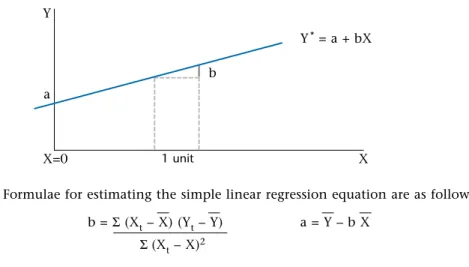
The form of the simple linear equation is: Y*= a + b
1X1
where:a = the intercept term (the point at which the line crosses the Y axis or where X = 0)
b = the slope coefficient. As X increases 1 unit, Y*increases by b units.
If b is negative, the equation will be that of a negatively-sloped line—that is, as X increases, Y*will decrease.
Formulae for estimating the simple linear regression equation are as follows: b = Σ(Xt– X) (Yt– Y) a = Y – b X
Σ (Xt– X)2
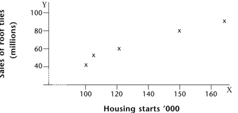
Example: Assume that the sales of a particular type of CSR roof tile is dependent on the number of housing starts in the preceding half year. Other factors of potential importance will be ignored in this simple equation. The following (fictitious) data shown in Figure 2 might be considered, and are represented graphically in Figure 3.
Figure 1 A theoretical regression line showing the role of the slope and intercept
Figure 2 Hypothetical data for CSR roof tile sales
PERIOD X = HOUSING STARTS IN Y = SALES OF CSR
PRECEDING HALF YEAR ROOF TILES
(THOUSANDS) (MILLIONS) 1 100 43 2 112 54 3 165 91 4 150 80 5 121 60 Y*= a + bX Y X=0 1 unit X a b SIMPLE REGRESSION MODEL
A regression model with only one independent variable
The regression involves a number of intermediate calculations, the detail of which is shown in Figure 4.
This provides us with the final equation:
Y*= –27.95 + 0.7218 X
which can be interpreted as:
b = 0.7218
This means that for every 1 unit of X (every 1000 housing starts), sales of roof tiles will = 0.7218 units of Y (0.7218 x 1 million roof tiles = 721 800 roof tiles).
a = –27.95 has a less significant meaning, being negative. This sometimes happens in a mathematical regression equation, with a positively-sloped line.
This is an example based on fictitious data, but it serves to show the workings of a regression equation. In the real world of business, the tedium of such calculation is removed by the use of statistical and forecasting computer software, such as SPSS, Microtab, TSP and Forecast-Pro.
Figure 3 Graphical representation of data Figure 4 Intermediate regression calculation Y X 100 120 140 150 160 40 60 80 x x x x x 100
Sales of roof tiles
(millions) Housing starts ’000 PERIOD X X – X (X – X)2 Y Y – Y (X–X) (Y–Y) 1 100 –29.6 876.16 43 –22.6 668.96 2 112 –17.6 309.76 54 –11.6 204.16 3 165 35.4 253.16 91 25.4 899.16 4 150 20.4 416.16 80 14.4 293.76 5 121 –8.6 73.96 60 –5.6 48.16 ΣX = 648 Σ(X–X)2 ΣY = 328 Σ(X–X)(Y–Y) X = ΣX/n = 2929.2 Y = ΣY/n = 2114.2 = 648/5 = 328/5 = 129.6 = 65.6 b = Σ(Xt– X) (Yt– Y) = 2114.2 = 0.7218 Σ(Xt–X)2 2929.2 a = Y – bX = 65.6 – (0.7218)129.6 = 65.6 – 93.55 = –27.95
Many more statistics can be calculated in relation to regression analysis, which enables hypotheses to be tested relating to the importance of variables used in the equation and to the overall value of the equation as a whole. However, as with any complex statistical methodology, caution must be used in the design, conduct and analysis, as incorrect initial assumptions can invalidate the entire process. Nonetheless, in the hands of experienced and knowledgeable users, and with the use of increasingly available and sophisticated computer technology, regression techniques provide a useful quantitative basis for many business forecasts. Further details of regression analysis can be obtained from statistics or econometric textbooks.
COMBINATION OF TIME SERIES
AND REGRESSION ANALYSIS
As mentioned above, simple regression involves a regression model with only one depen-dent variable. However, this is often too simplistic to tell the entire story. Astute use of multiple regression requires much skill in selecting appropriate variables and in main-taining the statistical validity of the more complex relationship. Sometimes forecasters substitute timefor multiple independent variables in a regression equation as a proxy for a multitude of other variables.
The following example, using quarterly champagne sales (fictitious data), shows how time series analysis and regression analysis can be used to create a forecast, with the addi-tion of seasonal indices. The steps are as follows:
1. Compilation of the appropriate background data. This method assumes that at least ten periods of data are available. In this example we have chosen to use quarterly data. This data is shown as the sales column in Figure 5.
2. Smoothing of data to form an approximate trend, from which the seasonal indices can eventually be defined. This procedure commences with the calcula-tion of a four-quarter moving total, then the calculacalcula-tion of a centred moving total, which is then divided by four to give a centred moving average. The four period moving average can be used as a trend in its own right. These calculations are shown in Figure 5 (four-quarter MT, centred MT and centred MA columns). 3. The final column of Figure 5 shows the index (sales/CMA). Values below 100
show that sales are less than the centred moving average, and vice versa. Figure 6 summarises the index column from Figure 5, and calculates the average index for each of the respective quarters. A final adjustment ensures that all four indices add up to 100. A quick check of the dimensions of these seasonal indices con-firms the expected seasonal pattern of champagne sales, with the highest index value occurring in quarter IV—the festive season.
4. Calculation of regression equation: sales = function (time). The result is shown in Figure 7.
5. Application of seasonal indices to projected trend line to produce forecast for next eight quarters. Figure 8 shows the workings of this, while Figure 9 provides a graphical representation of the sales and forecast.
Figure 5
Fictional data of sales of a champagne product in A$ million.
Figure 6
Calculation of seasonal index (using index column from Figure 5)
KEY MT = moving total MA = moving average
CMA = centred moving average SI = seasonal index
T = trend
PERIOD SALES FOUR-QUARTER CENTRED CENTRED INDEX
MT MT MA SALES/CMA Year 1 Quarter I 0.8 II 1.3 III 1.4 5.8 6.1 1.525 91.8 IV 2.3 6.4 6.5 1.625 141.54 Year 2 Quarter I 1.4 6.6 6.9 1.725 81.16 II 1.5 7.2 7.6 1.9 78.95 III 2.0 8.0 8.0 4.0 50 IV 3.1 8.0 8.15 2.04 151.96 Year 3 Quarter I 1.4 8.3 8.45 2.11 66.35 II 1.8 8.6 8.85 2.21 81.44 III 2.3 9.1 9.4 2.35 97.87 IV 3.6 9.7 10.35 2.59 139.0 Year 4 Quarter I 2.0 11.0 11.75 2.94 68.03 II 3.1 12.5 12.85 3.21 96.57 III 3.8 13.2 IV 4.3 Quarter I II III IV 91.80 141.54 81.16 78.95 50.00 151.96 66.35 81.44 97.87 139.00 68.03 96.57 Average 71.85 85.65 79.89 144.16 Adjusted Final SI 75.33 89.79 83.75 151.13 Total = 400
Calculation of regression trend
Let Y = Sales data as above Let X = Time from 1 to 16
Using a regression equation fitted to the above data: Y*= 0.7787 + 0.1738 t
The interpretation of the b value of 0.1738 is that for every increase in time period, sales will increase by 0.1738 million dollars or $173,800.
Figure 7
Calculation of regression trend for champagne sales forecast
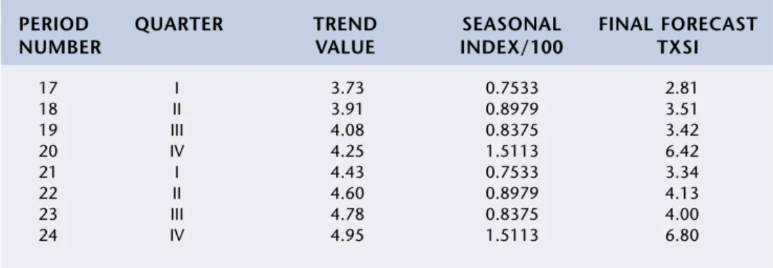
Let us now assume that we wish to forecast two years into the future beyond the given data. Given that our data stops at period 16, we will wish to be forecasting sales for periods 17 to 24. Thus in the equation Y*= 0.7787 + 0.1738t, we will be substituting
pro-gressively the values t = 17, t = 18...t = 24 to get the trend base of the forecast. We will then multiply this by the seasonal index to obtain the final forecast.
It is important to note that this method presupposes that a sufficiently long sales his-tory exists to be able to develop a seasonal index, and that pre-existing conditions will hold for the next eight periods. In reality this may not be so, but this statistical forecast base can then be adjusted for the findings of qualitative research. The overlay of a cycli-cal effect may also be necessary. However, despite the fact that such techniques might have some shortcomings, they are usually much more satisfactory than pure ‘guessti-mates’. In practice, adjustments to forecasts obtained through quantitative methods may be made on the basis of more qualitative methods. Some of these will now be discussed.
EXPERT OPINION
At times, forecasts may be made with little formal statistical analysis, relying instead on the use of experienced judgment by executives, marketing consultants, trade associations, buyers/sellers or academics.
Forecasts made by executives may be based on intuition rather than scientific methodology. Their success probably depends on the degree of insight into the overall market behaviour of the particular executive. In a large organisation, reliance on such judgment without the backup of more rigorous methods may prove to be risky in the long term, especially in a fluid competitive environment.
Forecasts made by in-market contacts, such as customers, distributors, dealers or wholesalers, may also suffer from anticipation bias, whereby sales estimates are inflated in anticipation of unrealistically high future business.
Figure 8 Combining regression trend and seasonal indices to create final forecast
Figure 9 Graphic representation of original sales, and forecast
PERIOD QUARTER TREND SEASONAL FINAL FORECAST
NUMBER VALUE INDEX/100 TXSI
17 I 3.73 0.7533 2.81 18 II 3.91 0.8979 3.51 19 III 4.08 0.8375 3.42 20 IV 4.25 1.5113 6.42 21 I 4.43 0.7533 3.34 22 II 4.60 0.8979 4.13 23 III 4.78 0.8375 4.00 24 IV 4.95 1.5113 6.80 Actual Year 1 2 4 6
Year 2 Year 3 Year 4 Year 5 Year 6
Sales in $million ➤ ➤ ➤ ➤ Forecast
Independent expert opinions from marketing consultants, academics or trade associa-tions are also worthwhile obtaining because of their specialist skills and database access. However, even experts can be wrong, especially if they are not in close contact with ‘the real world’. One precautionary approach used, especially for particularly critical forecasts, is a jury of expert opinion, whereby a consensus of opinion is reached from the opinions of several experts, each with different spheres of expertise or experience. For example, the views of the marketing executives, economists, software research and development experts and Bill Gates himself may be merged to help to ascertain the forecast demand for Microsoft products in forthcoming periods. One such approach, coined the Delphi technique, involves gathering managers’ and others’ opinions independently, validating them centrally, and progressively refining them in successive rounds until consensus is reached. The Delphi method avoids many weighting and judgmental problems, with the median of the groups’ overall responses forming the final forecast. The approach is particularly useful for new product forecasts when no historical information is available on which to base a forecast. Overall, however, expert opinion should not be used in isolation, but as a complement to quantitative techniques.
SALES FORCE OPINIONS AND
CUSTOMER OPINIONS
Two other sources of market opinion are often sought in the forecasting process. These are sales force opinions and actual/potential customer opinions.
The opinions of salespeople should be considered to some extent, as they are at the forefront of the market and in an ideal position to assess customer reactions and com-petitors’ activities. Their estimates are especially useful in some business markets where the customers may be well-known to the salespeople and where relatively few customers dominate the market. Good retail sales assistants opinions should also not be ignored. However, salespeoples’ estimates should be used with caution. They are often based on a relatively narrow perspective of the entire market, with little consideration of broader economic trends or even of wider policy effects from within the organisation. Certain biases may also be present in salespeoples’ estimates, either because of their personal opti-mism or pessiopti-mism or because of their short-term emphasis on recent successes or failures in the marketplace. There is also a risk that that they may underestimate demand in order to be allocated low sales quotas, which form the benchmark for the payment of bonuses. Salesperson representation in the jury of expert opinion provides a two-way benefit, not only through receipt of their opinion, but also in their appreciation of having their opinion valued. This, combined with the payment of salaries to salespeople with reduced emphasis on bonuses, acts as an incentive for salespeople to provide accurate estimates.
Actual or potential customer opinioncan be ascertained via the market research process. Surveys and panel analysis of opinions of past, current and potential customers, along with surveys or focus group research of retailers, wholesalers, agents and other gatekeep-ers, can help to identify what is happening in different market segments. This sort of activity is particularly necessary in a dynamic market.
Surveys are sometimes combined with market testswhen the company wants to esti-mate customers’ reactions to possible changes in its marketing mix. Pricing experiments, new product testing and even advertisement testing can often be undertaken in an economical way in a small test market. Such tests may simply involve a measurement of likely demand for a product the marketing mix of which is almost finalised. Alternatively, it may involve some actual experimentation with pricing or promotion strategies.
JURY OF EXPERT OPINION
When consensus of opinion is reached from the opinions of several experts
THE DELPHI TECHNIQUE
The independent gathering of managers’ and others opinions, their central validation and reinforcement in successive rounds until consensus is reached