The Exploration of Cross-Sectional Data with
a Virtual Endoscope
William E. Lorensen, MS
GE Corporate Research and Development, Schenectady, NY
Ferenc A. Jolesz, MD Ron Kikinis, MD
Brigham and Women’s Hospital, Boston, MA
Abstract. Endoscopes provide real-time, high resolution video views of the interior
of hollow organs and cavities that exist within the human body. Although endoscopic examinations are mostly non-invasive, the procedures still require some sedation or anesthesia to reduce patient discomfort. X-Ray Computed Tomography (CT) and Magnetic Resonance Imaging (MRI) are non-invasive diagnostic imaging techniques that display internal anatomy in cross sections called slices. For the most part, radiol-ogists view the 2D cross sections and create mental images of the 3D structures present in the study. However, many of the tubular structuresthat exist in the body have complex morphology, passing back and forth through the cross sections. This paper illustrates techniques for the internal exploration of CT / MRI data that have been reconstructed into 3D surfaces. The views produced by the new methods simu-late the types of views that can be obtained with endoscopes. Examples from the brain, cranium, chest, and abdomen illustrate the techniques.
1. Introduction
Endoscopes provide real-time, high resolution views of the interior of hollow organs and cavities that exist within the human body. Although an endoscopic examination is mostly non-invasive, the procedures still require some sedation or anesthesia to reduce patient dis-comfort. X-Ray Computed Tomography (CT) and Magnetic Resonance Imaging (MRI) are non-invasive diagnostic imaging techniques that display internal anatomy in cross sections called slices. For the most part, the radiologist can view the 2D cross sections and create a mental image of the 3D structures present in the study. However, many of the tubular struc-tures that exist in the body have complex morphology, passing back and forth through the cross sections.
Traditionally, radiologists view the 2D slices or 3D compositions of the slices from the outside looking in while endoscopists view the organs from the inside. We have developed techniques that provide both types of views for the exploration of CT / MRI data that have been reconstructed into 3D surfaces. The internal views produced by the new methods sim-ulate the types of views that can be obtained with endoscopes. Compared with real endo-scopic views, the virtual endoscope has the following advantages:
1. Interactive control of all virtual camera parameters including the field-of-view. 2. Ability to pass through the walls of the organ to view neighboring anatomy.
4. User controlled movement along a computer generated path. 5. An infinite depth of field.
We have developed two approaches to generate camera paths through 3D surface models created from CT / MRI data. The first uses a computer animation technique called key fram-ing. Using camera controls on a graphical user interface, an operator moves the virtual cam-era to “key” locations in and / or around the organ being explored. All parameters of the camera are under user control. Once the key frames have been established, the system fits a smooth cubic spline through each parameter and generates a flight path. The second approach uses robot path planning algorithms to automatically find a path through a pas-sage. The user specifies a final goal for the camera and the system labels all regions in the 3D volume with its distance to the goal. Any locations in space occupied by “obstacles” are by-passed. Then, from a user selected starting point, the system generates a smooth flight path to the goal.
For both techniques, once the path is generated, the user can start, stop and step along the calculated path. We also describe several visualization alternatives including: split screen views of the 3D endoscope and 2D slices, split screen views of the 3D endoscope and a “bird’s eye” view of the same anatomy, an interactive “where am I?” facility, and stereo viewing.
2. The Virtual Endoscope
The virtual endoscope consists of several subsystems:
1. An image acquisition system capable of producing cross sectional images of internal anatomy. In this paper we use both X-ray Computed Tomography (XRAY-CT) and Mag-netic Resonance Imaging (MRI) systems to generate the cross sections.
2. A segmentation toolkit that identifies tissues of interest within the three-dimensional vol-ume described by the cross sectional images.
3. A surface extractor that builds polygonal models of each selected tissue.
4. A path finder that calculates a “safe” trajectory through an organ selected by the user. 5. A renderer capable of transforming and manipulating a polygonal data set.
2.1 Image Acquisition
Modern medical XRAY-CT and MRI systems can rapidly acquire cross-sectional data. By acquiring multiple, contiguous 2D cross-sections, both modalities can produce a volume that covers a 3D field-of-view.
CT measures the spatially varying X-ray attenuation as the X-ray beam passes through the anatomy. Different tissues absorb different amounts of energy, producing, after process-ing, an image with varying intensities. CT is usually used to visualize bone and organ / air boundaries although injected contrast can enhance soft tissues. Helical and spiral CT sys-tems acquire data continuously as the patient is moved on a table, covering large areas in relatively short acquisition times, allowing the imaging of organs that remain still during a patient breath hold.
MRI systems measure the relaxation of nuclear spin magnetization. The reconstructed images reflect the differing relaxation times of different tissue. MRI can image soft tissue of relatively stationary organs such as the brain. MRI can also measure flow.
2.2 Segmentation Toolkit
After acquiring image data that covers the anatomy of interest, the first step towards a sur-face is segmentation. The imaging modality and anatomical location of the study dictate the choice of segmentation. Regardless of the segmentation technique, the goal of the process is to identify the tissue of the voxels in the dataset. For the virtual endoscope, we use the fol-lowing techniques:
• Thresholding - a voxel is classified based on the signal in the original data. For example, for computed tomography, voxels with a Hounsfield number equal to 200 are considered bone, while those below -400 are considered air.
• Thresholding with connectivity - voxels that are connected to initial seed voxels and that also satisfy a threshold criterion are marked with a unique tissue identifier [1]. Magnetic Resonance Angiography (MRA) flow images are suitable for this segmentation tech-nique. The bronchial tree in the lungs can also be extracted using connectivity and thresh-olding.
• Two channel segmentation - simultaneously acquired signals from two images can be used to create tissue masks. These techniques use a variety of statistical classification algorithms [2] including non-parametric, nearest neighbor and parzen windows [3]. These two channel data sets are readily acquired on MRI systems. When only one chan-nel of data is available (such as Fast Spin Echo MRI or CT), a second, synthetic chanchan-nel can be derived from the gradient of the acquired data. The two channel segmentation technique has been used on over 1000 cases as part of a multiple sclerosis progressive study.
• Morphological operators - parts of the anatomy that touch other parts with the same threshold signals provide the greatest segmentation challenge. Here we find that applica-tion of thresholding and two channel techniques followed by interactive erosion / dilaapplica-tion operators [4] isolate most tissues. We have used this technique to segment organs in the abdomen [5].
• For some cases, none of the above segmentation techniques can label the tissues of inter-est. Here we use an interactive slice labelling tool to complete the segmentation.
2.3 Surface Extractor
Once the voxels in the image dataset are labeled with tissue / organ identifiers, we extract surfaces consisting of triangles using the marching cubes algorithm [6]. Marching Cubes locates triangles that lie on the surface of an identified tissue using linear interpolation to locate the tissue boundary within a “cube” defined by eight neighboring voxels. A surface orientation is also derived for each triangle vertex from the gradient of the voxel data. For the endoscopic application, triangles are preferred over points or direct volume renderings because the simulated endoscope will be close to the extracted surfaces and re-interpolation of the volume data is too computationally expensive for the desired interactive rendering speeds. Because a large numbers of triangles are often required to model the surfaces, we usually reduce the number of triangles in relatively flat portions of the surface using a trian-gle decimation algorithm. The decimated triantrian-gle lists can improve rendering speeds with some loss of detail [7].
2.4 Camera Control
We use three techniques to guide a virtual camera through the surface models.
1. Users control the camera with a mouse. The controls permit the movement of the camera about its focal point or its position. We also control the field of view of the camera. The manual technique is best suited for applications like surgical planning and surgical simu-lation.
2. Users select “key points” along a desired camera trajectory. This keyframing is a com-mon computer animation technique that interpolates between the selected points. Cubic splines [8] can be used to calculate intermediate parameter values at any desired resolu-tion. Keyframing is suitable for gross camera movements through open interior and exte-rior environments. We select the “key” camera location and orientation values using manual camera movement.
3. Traversal through the hollow organs that we wish to explore with the virtual endoscope present a challenge for techniques 1) and 2). Manual camera movement in confined spaces is difficult. To guide our virtual endoscope, we have adapted a robot path planning algorithm [9].
2.5 Path Planning
The path finding algorithm consists of two steps. First we calculate a “navigation volume” as follows:
1. The user selects a goal point interactively on a cross sectional image.
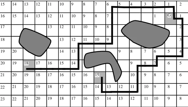
2. We calculate the distance to this point from each voxel in the study using a wavefront propagation algorithm. This path planning assumes the robot is a point. Any voxels that have an intensity within a user specified range are considered obstacles and are not labelled. Figure 1 shows the distance labelling for a single slice. The goal is point G. The
G 1 1 1 2 2 2 3 3 4 4 5 5 6 6 7 7 7 5 6 7 8 8 8 7 6 7 8 8 8 8 8 9 9 9 9 9 9 9 9 9 10 10 10 10 10 10 10 11 11 11 11 11 11 12 12 12 12 12 12 13 13 13 13 13 13 13 14 14 14 14 14 14 15 15 15 15 15 15 15 16 16 16 16 16 16 17 17 17 17 17 18 18 18 18 18 19 19 19 19 19 20 20 20 20 20 21 21 21 22 22 23
current implementation uses a manhattan (city block) distance for efficiency. Each voxel in the navigation volume has an integer distance to the goal. Voxels containing obstacles are not labelled. The distance labelling terminates when no new neighbors of the wave-front can be labelled.
Once the navigation volume is created, we display the slices of this volume as though they were anatomical slices.
1. The user points to a location on a navigation volume slice and the system reports the dis-tance to the goal if one exists. We normally select the goal at the terminus of the organ to be explored. A path from any labelled point in the volume to the goal is calculated using a steepest descent algorithm. Figure 2 shows the calculated paths from two starting points
in the two-dimensional example.
2. The points along the path from a starting point to the goal are converted into a smooth path using the keyframing facility outlined above. Because the algorithm generates small steps as it moves towards the goal, we often decimate the points on the path by a factor of two or three before interpolating them.
2.6 Display
With the surface models of the desired anatomy and a path (or means to generate one), we use a variety of display techniques to present endoscopic-like views of the cross-sectional data:
1. Single 3D image - this is traditional surface rendering. The triangle lists of the organs can be readily rendered using commercial polygon acceleration hardware. Transparent ren-derings of large enclosing tissue (such as the skin) allow an unobstructed view of the interior while providing a three-dimensional context for the user.
FIGURE 2. Two paths to reach goal G.
G 1 1 1 2 2 2 3 3 4 4 5 5 6 6 7 7 7 5 6 7 8 8 8 7 6 7 8 8 8 8 8 9 9 9 9 9 9 9 9 9 10 10 10 10 10 10 10 11 11 11 11 11 11 12 12 12 12 12 12 13 13 13 13 13 13 13 14 14 14 14 14 14 15 15 15 15 15 15 15 16 16 16 16 16 16 17 17 17 17 17 18 18 18 18 18 19 19 19 19 19 20 20 20 20 20 21 21 21 22 22 23
2. Stereo - we routinely use stereoscopic viewing to enhance the perception of three dimen-sional relationships. We use three different types of stereo display hardware: NTSC video tapes viewed with LCD shutter glasses (3D TV Systems. San Rafael, CA), high resolu-tion workstaresolu-tion display viewed with LCD shutter glasses (StereoGraphics, San Rafael, CA) and large screen projection using polarized glasses (VREX, Hawthorne, NY). All three techniques require two separate images: one corresponding to the left eye view and one corresponding to the right eye view.
3. Split screen - we present two views simultaneously. One is a view from a user specified location that serves as a localizer for the endoscope. This overview uses a geometric clip-ping technique to cut a hole through any anatomy between the overview camera and the endoscopic camera [10].
4. Where am I? - while moving along the generated path, the user can press the “Where am I?” button that changes to the overview with a pointer showing the location of the endo-scope.
5. Camera tracking on cross-sectional slices - an auxiliary window shows the location of the endoscope as a marker on the original CT or MRI slices. This localizes the endoscope within the familiar cross-sectional image.
3. Results
We tested the feasibility of the virtual endoscope on four regions of the anatomy. The exam-ples illustrate a variety of imaging modalities, path planning and presentation.
3.1 Cranium
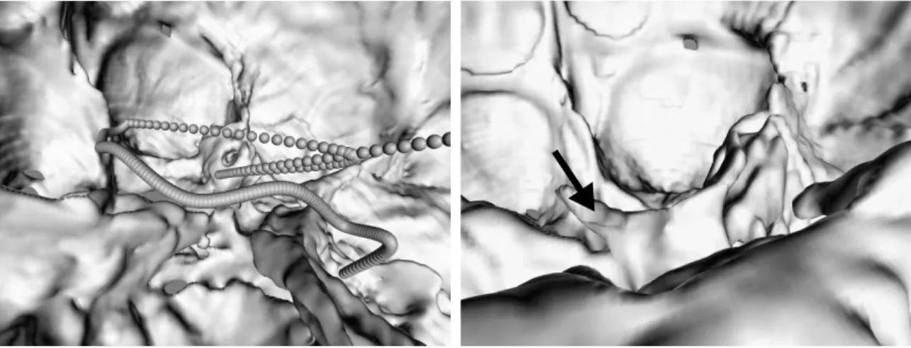
This CT study contains 95 slices with a 24 cm field of view. The pixels are .46875 mm’s square with 1.5 mm between slices. The skin and bone were segmented using connectivity to remove the head holder. Running marching cubes on the study with Hounsfield number of -400 produced a skin surface. The bone was extracted using a Hounsfield number of 200. The resulting surfaces contained 411,000 and 985,000 triangles respectively.We decimated the skin surface to improve rendering performance. One decimation iteration removed 300,000 triangles. In this example we simulated an endoscope passing through the paranasal
the nostril, passing into the paranasal sinuses into the cranium. Figure 3 shows part of the interpolated flight path as a string of spheres. Figure 4 shows a view inside the cranium looking towards the rear. The arrow points to the clinoid process of the clivus.
3.2 Vessels in the Brain
This phase contrast MRI study of the vasculature in the head illustrates a split screen display to facilitate localization of the endoscope. The study produced .78125 mm pixels, 1 mm apart. The vessels were extracted using connectivity and thresholding. The cut away reveal-ing the location of the camera used boolean texture maps [10]. Two boolean clippers, one an elliptic cylinder, the other a plane were used. One end of the cylinder was keep at a constant view location while the other remained pointed at the position of the virtual endoscope. The endoscopic view, cutaway view and overviews in Figure 5 were rendered into separate viewports and updated simultaneously.
3.3 Aorta
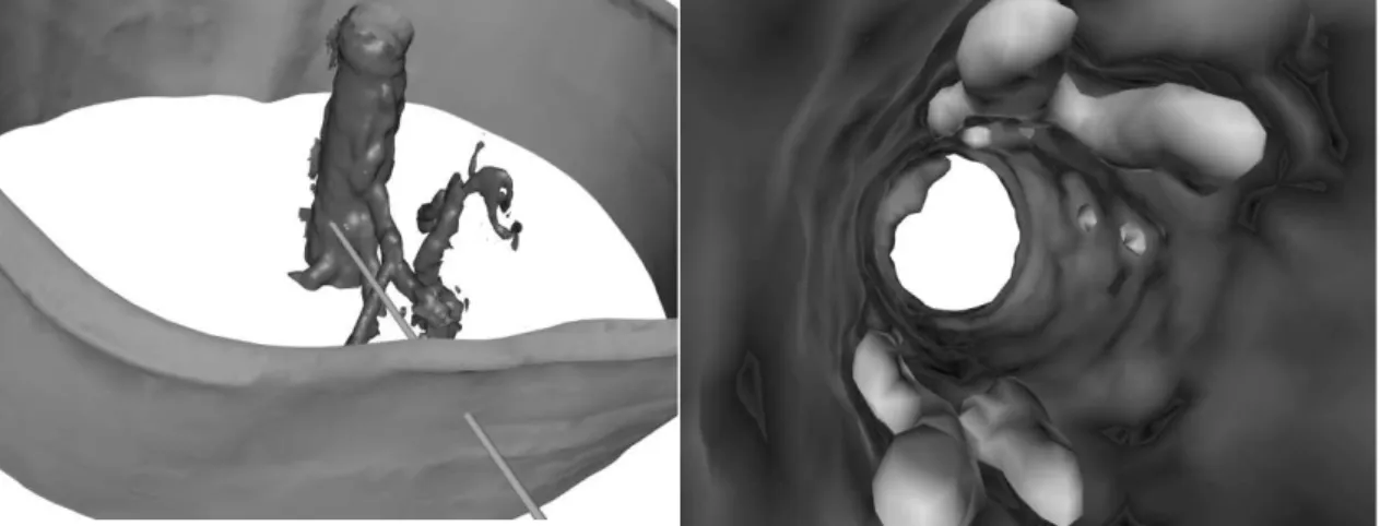
A CT study of the chest reveals plaque in the aorta. The sixty 3 mm slices were obtained fol-lowing the injection of contrast material. Multiple connectivity seeds were necessary to
FIGURE 5. Multiple views of the vessels.
FIGURE 6. The aorta viewed from outside. The cylinder shows the
location of the camera.
FIGURE 7. A look at the aorta from within showing the plaques.
extract the separated plaques. Figure 6 shows an external view of the aorta with a cylinder pointing through the skin and to the current endoscope location. Figure 7 shows the interior as seen by the virtual endoscope, showing the lighter plaque surfaces and their relationship to the wall of the aorta.
3.4 Colon
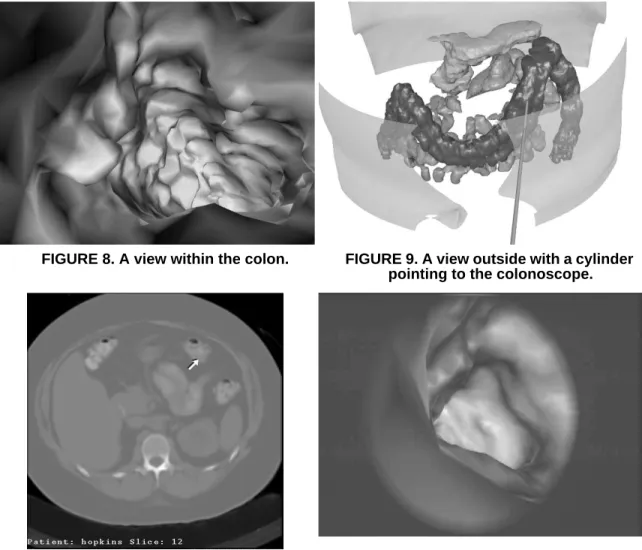
A CT study of the colon tested the versatility of our segmentation toolkit. The colon, pan-creas and small intestine were identified using morphological operators, connected compo-nents and hand labelling. The surface of the colon is represented with 60,000 triangles. Figure 8 shows a view within the colon. For interior views, we do not decimate the models. At anytime during the flight, the user can press a button to show the location of the camera. Figure 9 shows the location of the camera corresponding to the internal view. In this local-ization view, we decimated the skin, pancreas and small intestine models to improve render-ing performance. Figure 10 shows a pointer to the current 3d location on a cross section. This location is updated interactively while the colonoscope moves along the calculated
FIGURE 8. A view within the colon. FIGURE 9. A view outside with a cylinder
pointing to the colonoscope.
FIGURE 10. The corresponding cross-section with an arrow pointing to the
colonoscope.
FIGURE 11. A frame of video from the virtual colonoscope.
4. Conclusions
A Virtual Endoscope can provide endoscopic-like views of the interior of hollow organs extracted from cross-sectional images. The technique is non-invasive, requiring no patient anesthesia. The endoscope can be controlled manually or travel along paths generated using keyframing or robot motion path planning. A variety of visualization techniques aid the viewer’s localization of the virtual endoscope.
This paper has emphasized the algorithmic issues involved in creating a virtual endo-scope, leaving the clinical aspects of the problem to future work[11]. These initial results are encouraging but the clinical efficacy of the technique needs to be established. Work is already underway to verify the visual and quantitative results. This validation is being per-formed on phantoms designed for CT and MRI. Also, image acquisition protocols custom-ized for specific regions of anatomy are being developed.
Additional algorithmic work is also necessary. We continue to develop more robust and efficient segmentation algorithms. Our goal is to provide organ-specific segmentation tech-niques that require no user interaction. Also, the path planning algorithm is being extended to establish paths that travel down the centers of the organs. The current method creates paths that tend to ride the interior surface. We are extending the path finding to take into account the size of the virtual endoscope. Geiger [12] reports a path finding technique for an endoscope that uses finite element techniques to guide a camera of a specified size through hollow organs. Our extended work, based on robot path planning techniques, follows the work of Barraquand [13].
References
[1] Cline, H. E., Dumoulin, C. L., Lorensen, W. E., Hart, H. R., and Ludke, S., “3D Recon-struction of the Brain from Magnetic Resonance Images Using a Connectivity Algo-rithm,” Magnetic Resonance Imaging, vol. 5, no. 5, pp. 345-352, 1987.
[2] Cline, H. E., Lorensen, W. E., Kikinis, R., and Jolesz, F., “Three-Dimensional Segmen-tation of MR Images of the Head Using Probability and Connectivity,” Journal of
Com-puter Assisted Tomography, vol. 14, no. 6, pp. 1037-1045, November/December 1990.
[3] Duda, R. O. and Hart, P. E., in Pattern Analysis and Machine Intelligence, ed. Wiley Interscience, pp. 92-93, New York, 1973.
[4] Serra, J., “Introduction to Mathematical Morphology,” Computer Vision, Graphics and
Image Processing, vol. 35, no. 3, pp. 283-305, September 1986.
[5] Silverman, S. G., Kikinis, R., Chernoff, D. M., Adams, D. F., Seltzer, S. E., and Lough-lin, K. R., Three dimensional Imaging of the Kidneys using Spiral CT: A Potential Sur-gical Planning Tool, p. 136, RadioloSur-gical Society of North America, Chicago, IL, December 1992.
[6] Lorensen, W. E. and Cline, H. E., “Marching Cubes: A High Resolution 3D Surface Construction Algorithm,” Computer Graphics, vol. 21, no. 3, pp. 163-169, July 1987. [7] Schroeder, W. J., Zarge, J., and Lorensen, W. E., “Decimation of Triangle Meshes,”
Computer Graphics, vol. 26, no. 2, pp. 65-70, August 1992.
[8] Kochanek, D. H. U. and Bartels, R. H., “Interpolating Splines with Local Tension, Con-tinuity, and Bias Control,” Computer Graphics, vol. 18, no. 3, pp. 33-41, July 1984. [9] Lengyel, J., Reichert, M., Donald, B. R., and Greenberg, D. P., “Real-Time Robot
Graph-[10] Lorensen, W. E., “Geometric Clipping with Boolean Textures,” in Proceedings of
Visu-alization ‘93, pp. 268-274, IEEE Press, October 1993.
[11] Jolesz, F. A., Lorensen, W. E., Kikinis, R., Saiviroonporn, P., Seltzer, S., Silverman, S., Philips, M., Geiger, B., “Virtual Endoscopy: Endoscopy-like Viewing and Exploration of Three Dimensional Image Data,” submitted to Radiology, November 1994.
[12] Geiger, B. and Kikinis, R., “Simulation of Endoscopy,” in AAAI Spring Symposium
Series: Applications of Computer Vision in Medical Image Processing, pp. 138-140,
Stanford University, 1994.
[13] Barraquand, J., Latombe, J., “Robot Motion Planning: A Distributed Representation Approach,”, The International Journal of Robotics Research, vol. 10, no. 6, pp. 628-648, December 1991.