* Research supported in part by KBN Grant No. PBZ KBN 016/P03/1999.

PROBABILrn AND

MATHEMATICAL STATISTICS Vol. 24, Fsgc 1 (2W4), pp 1-15

ON ANNUITIES UNDER RANDOM RATES OF INTEREST'

WITH PAYMENTS VARYING

IN

ARITHMETIC

A N D GEOMETRIC PROGRESSION BY

K. BURNECKI*, A. M A R C I N I U B AND A. WERON* (WUOCLAW)

Abstract. In the article we consider accumulated values of an- nuities-certain with yearly payments with independent random interest rates. We focus on general annuities with payments varying in arith- metic and geometric progression which are important varying annui- ties. We derive, via recursive relationships, mean and variance for- mulae of the final values of the annuities. Special cases of our results correct main outcome of Zaks [4].

Mathematica Subject Classification: 91B28, 91370.

Key words and phrases: Annuity, accumulated value, random interest rate.

1. INTRODUCTION

An annuity is defined as a sequence of payments of a limited duration which we denote by n (see, e.g., Gerber [2]). The accumulated or final values of annuities are of our interest. Typically, for simplicity, it is assumed that under- lying interest rate is fixed and the same for all years. However, the interest rate that will apply in future years is of course neither known nor constant. Thus, it seems reasonable to let interest rates vary in a. random way over time, cf. e.g. Kellison [3].

We assume that annual rates of interest are independent random variables with common mean and variance. We apply this assumption in order to com- pute, via recursive relationships, fundamental characteristics, namely mean and variance, of the accumulated values of annuities with payments varying in arithmetic and geometric progression. These important varying annuities can be reduced to the cases considered by Zaks [4].

In Section 2 we introduce basic principles of the theory of annuities. Under the fixed interest assumption we consider accumulated values of stan-

2 K. Burnecki et al.

dard and non-standard annuities. Finally, we introduce the ones with pay- ments varying according to arithmetic and geometric progression. It appears that all important types of annuities (cf. Kellison [3]) can be obtained as examples of the introduced ones.

In Section 3 we drop the assumption of fixed interest rates and we study the find values of the varying payment annuities under stochastic approach to interest. We consider annual rates of interest to be independent random varia- bles with common mean and variance. Using recursive relations we compute the first and second moment as

well

as variance of the accumulated values. Special cases of the derived results correct main outcome of Zaks [4], which was pointed out in. Burnecki et al.

[I].

In Section 4 we illustrate variance results comparing them with computer approximations obtained by

means

of the Monte Carlo method.

2. ANNUITIES UNDER FIXED INTEREST RATES

First let us recall basic notation used in the theory of annuities. Suppose that j is a positive annual interest rate and fixed through the period of n years. The annual discount rate d is given by the formula

and the annual discount factor v is given by the equation

Hence we have

In the article we concentrate on final or accumulated values of annuities. We assume that k

<

n throughout, unless otherwise specified. The accumulated value of an annuity-due with k annual payments of 1 is denoted by i.qj and given by the formulae

and

( 5 ) i~~~ = (l+j)k+(l+j)k-l+...+(l+j) = (l+j)(l++ilj),

where the latter defines the recursive equation for iElj.

Let us now consider a standard increasing annuity-due. The accumulated value of such an annuity with k annual payments of 1, 2,

. . .

,

k, respectively, is

Annuities under random rates of interest

3

The accumulated value of un increasing annuity-due with k annual pay- ments of 12, Z2,

. .

.,

k Z , respectively, is denoted by

(I2

s ) ~ ~ and calculated by the formula

The following two equations give the recursive formula for (12shlj and set the relationship between (12Shlj and &lj:

The latter corrects Corollary 2.1 from Zaks [4].

In the sequel we will need the following two relations:

Standard decreasing annuities are similar to increasing ones, but the pay- ments are made in the reverse order. The accumulated value of such an an- nuity-due with k annual payments of n, n- 1,

. .

.,

n-

k+

1, respectively, is de- noted by (Di)n,Alj and given by the formulae:

and

The sum of a standard increasing annuity and its corresponding standard decreasing annuity is of course a constant annuity.

Now let us consider the accumulated value of an annuity-due with pay- ments varying in arithmetic progression (see, e.g, Kellison [3]). The first pay- ment is p and they subsequently increase by q per period, i.e. they form a se- quence (p, p + q , p + 2 q ,

.

. .,

p+(k- 1) q). We note that p must be positive but q can be either positive or negative as long as p

+

(k - I) q > 0 in order to avoid negative payments. The accumulated value of such an annuity will be denoted by and is defined by

4 K. Burnecki et al.

Important special cases are the combinations of p = 1 and q = 0, p = 1

and q = 1, and p = n and q = -1.

EXAMPLE 2.1. If p = 1 and q = 0, then ( S ~ ) $ ; ~ ~ becomes the acculnulated value of an annuity-due with k annual payments of 1, namely

(16) (5 a k l j )Q.W = $11.

EXAMPLE 2.2. If p = 1 and q = 1, then

(&)I;')

becomes the accumulated value of an increasing annuity-due with k annual payments of 1, 2 , . . ., k , respec- tively, namely

(17) ( i ) < l S l ~ a k l j = ( l 4 ~ ~ . j .

E X A ~ L E 2.3. I f p = n and q = -1, then ($$;) becomes the accumulated

value of a decreasing annuity-due with k annual payments of n, n- 1,

. .

.,

n - k

+

1, respectively, namely

f

18)

(s.)&

"

= (DS)jlj.

Let us finally consider the accumulated value of an annuity-due with k annual payments varying in geometric progression (see, e.g., Kellison [3]). The first payment is p and they subsequently increase in geometric progression with common ratio q ( q # l + j ) per period, i.e, they form a sequence

(PI pq, pq2, pq3,

. .

.,

pqk-I). W e note that p and q must be positive in order to avoid negative payments. The accumulated value of such an annuity will be denoted by (&)&I and is expressed as

(19) (5)gpq) s k l j = p ( ~ + j ) k + p q ( ~ + j ) k - 1 + p q 2 ( 1 + j ) k - 2 + ...+pqk-I( 1 + j )

Important special cases are the combinations of p = 1 and q = 1 (cf. Ex-

ample 2.1), and p = 1 and q = 1 +u, where u (u

+

j ) denotes a fixed rate of increase of the payments.

EXAMPLE 2.4. If p = 1 and q = 1, then (ig)$P) becomes the accumulated value of an annuity-due with k annual payments of 1, namely

(20) (s.)r_l.l) g klj = SElj.

.-

EXAMPLE 2.5. If p = 1 and q = 1 +u, then (ig)zy1 becomes the accumulated value of an annuity-due with k annual payments of 1 , 1

+

u, (1

+

u)',.

. .

,

(1

+

u ) ~ - ' , respectively. Moreover, it is easy to see that

Annuities under random rates of interest 5

3, ANNUITIES UNDER RANDOM INTEREST RATES

Let us suppose that the annual rate of interest in the kth year is a random variable ik. We assume that, for each

k,

we have E (ik) = j > 0 and Var (i,) = sZ, and that i l , i2,

.

..,

in are independent random variables. We write

(23) E ( l + i k ) = 1 f j = p and (24) E[(1+i32] = ( l + j ) 2 + s 2 = l + f = m, where (251 Obviously, (26)

Next we define r to be the solution of

and using (25) we have

For a k-year variable annuity-due with annual payments of c,

,

c,,

. . .

,

c,, respectively, we denote their final value by

Ck.

3.1. Payments varying in arithmetic progression. In the case of payments vary-

ing in arithmetic progression we have c, = p

+

(k

- 1) q, where k = 1 , 2 ,

. .

.,

n. The final value of an annuity with such payments is given recursively: (29)

ck

= ( l + i k ) [ ~ k - l + ( P + ( k - I ) q ) ] for k = 2, ..., n.

We can easily find pk = E (CA) as

(30)

~ ( c , )

= ~ ( ( 1

+&)

[ c k 1

+ ( P + ( ~ -

l)q)])

= ~ ( l + i ~ ) ~ ( ~ , - ~ + ( p + ( k - l ) q ) )

from independence of interest rates. Thus we have the recursive equation for k = 2,

. . .,

n:

We note that p, = p ( l + j ) = pp. The following lemma stems from (31) and (14).

6 K. Burnecki et al.

LEMMA 3.1. If Ck denotes the final value of an annuity-due with arznual payments uarying in arithmetic progression: p, p

+

q , p

+

24,

. . .

,

p

+

(k - 1) q, re- spectively, and if the

annual

rate of interest during the kth year is a random

variable ih such that E(1

+

ik) = 1 +j .and Var(1 +i,) = s2, and i l , i,,

. .

.,

i, are

independent random variables, then

Similarly, for the second moment E (Ci) we have the recursive equation for k = 2 ,

...,

n:

(33) mk = E(Ck2) = m [ m k - l + 2 ( p + ( k - l ) q ) p h - 1 + ( p + ( k - l ) q ) 2 ] .

We note that m1 = p2 m. In order to compute the second moment we need the following lemma.

LEMMA

3.2. Under the assumptions of Lemma 3.1 we

have

(34) mi^ =

MI^

+

2M2kI

where

(3 5 ) M I , = p2mk+(p+q)'mk-'+ ...+(p+(k-l)q)2m

and

(36) M2k = ( P + q ) m k - 1 ~ 1 + @ + 2 q ) r n k - 2 p 2 +

...

+

( ~ + ( k - l ) ~ ) m ~ ~ - ~ . P r o of. We proceed by induction. When k = 2, this follows on the equa- tion (33), since p1 = p (1

+

j ) = pp and m1 = p2 m. Assuming our result is true for a given k (2

<

k $ n- 1), it stems from formula (33) that it is also true for k

+

1. This concludes the proof by induction. a

Since, by (23), 1

+f

= rn, we can easily find that

(37) MI, = ~ ~ ~ ~ ~ ~ + 2 p q ( I ~ ] ~ ~ ~ + q ~ ( I ~ ~ ] ~ ~ f.

Now we can apply (10) and (11) in order to derive an equivalent expression for M I , .

LEMMA 3.3. We have

Now we shall determine M 2 , using [l5), (36) and the fact that 1

+f

= m.

Annuities under random rates o j interest 7

+2@+2q)(1 + f ) k p 2 + . . . + ( k - l ) ( p + ( k - l } q ) ( l + f ) ]

I

and applying (27) we obtain the following results.

LEMMA 3.4. Under the assumptions

of

Lemma 3.1 we have

LEMMA 3.5. Under the assumptions of Lemma 3.1 we have

~

I

I 1

(41) m* = ; i i [ ( q - ~ ) ( d @ - q ) ( l + ~ ) + 2 q v ) h - 2 q ( d ( p - q ) ( f + v ) + q v ) ( i i ) i l , I

We have thus reached a formula for E (Cz). In order to compute Var(Ck) we need yet an expression for E ( C , ) ~ .

LEMMA 3.6. Under the assumptions of Lemma 3.1 we have

+

- _{((Ii)';)zi;l - 2 ( 1}

+

kd)

j - k2).

(pi)'

Proof. It is easy to show that

$- - 2 6 (43) ( ~ z , j ) 2 = 2 k l l kII

d and

8 K. B u r n e c k i et al.

cf. Lemmas 3.3 and 4.3 from Zaks [4]. From (15) we may write

(45)

P:

=

((P

- 4)

G,j

+

4

(Wndl

2

= (p-4)' (j~lj)' +2q (4-P)

G1.j

(J$islj

+

q ( )klj-

Substituting from (43), (44) and (6) completes the proof, H Now, we are allowed to state the following theorem.

THEOREM

3.1. Under the assumptions of Lemma 3.1 we have

(46)

(ck)

= (ia)$),

(47) Var (C,) = m,

-

p i ,

where mk is given by Lemma 3.5, and

pz

by Lemma 3.6.

Let

us

now consider the situation when p = 1 and q = 0. We know, from

Example 2.1, that it is the case of an annuity-due with k annual payments of 1.

Then we obtain the following corollary, cf. Zaks [4].

COROLLARY 3.1. If

C k

denotes the

#nu1

value of an annuity-due with

k

an-

nual payments of 1 and

if

the annual rate of iilzterest during the kth year is a random variable i, such that E (1

+

ik) = I + j and Var (1

+

ik) = s2, and

.

,

21, a 2 ,

. .

.,

in are independent random variables, then

2(1 +j)k+1iElr-(2+j)iElf-(l +j)i3j4j+2(1 +j)GIj (49) Var (Ck) =

j

Another important case is the combination of p = 1 and q = 1, see Exam-

ple 2.2. It is an annuity-due with k annual payments of 1, 2,

. .

.,

k. The fol- lowing corollary is a direct consequence of Lemmas 3.1 and 3.3-3.5, cf. Burne- cki et al. [I].

COROLLARY 3.2. If

C k

denotes the final value of an increasing annuity-due with k annual payments of 1, 2,

.

. .,

k , respectively, and if the annual rate of interest during the kth year is a random variable ik such that E (1 +id = 1 + j and

Var(1 + i k ) = sZ, and il, i2,

..

.,

i, are independent random variables, then

(dl ink =

2 (1

+

j)k+Z (I~')E~, -2 (1 +j)

(likl

-j (2 +33 (12ili';)kl

j2

These results can be summarized in the following corollary, cf. Burnecki et al. [l].

Annuities under random rates of interest 9

COROLLARY 3.3. Under the assumptions of Corollary 3.2 we have

(51) Var (Ck) = 2 (1 +jIk+ (J$kIr -2 (1

+

j) ( J i l ~ ~ ~ - j

(2

+j) (12i)LlJ

j2 - (Ii]z, - 2 (1

+

kd)

-

k2

d2

Let

us

finally consider the situation when p = n and q = - 1, see Exam-

ple 2.3. Then we

obtain

the following corollary, cf. Burneclu et al. [I]. COROLLARY 3.4. If Ck denotes the final value of a decreasing annuity-due with

k

annual payments of n, n - 1, .

.

.

,

n-

k

+

1, respectively, and $ the annual rate of interest during the kth year is a random variable ik such that E (1

+

i,) = 1

+

j and Var (1

+

i,) = sZ, and ii

,

i2,

. . .,

in are independent random variables, then

(53) Var (Ck) = - iEll - 2 (n - l/jI2 (1 +j)k szl.

d2 l + r

-

1

+f

where 1 = (s/(l +j))2.

3.2. Payments varying in geometric progression. In the case of annuities-

due with payments varying in geometric progression we have ck = pqk-',

where k = 1, 2,

. .

.,

n. We assume that p and q are positive, q # 1 f j , q2 # 1

+

f

and q

St

l + r .

The final value of that annuity is given recursively:

As in the case of payments varying in arithmetic progression, we easiIy find that for k = 2, ..., n

The second moment E(C$ is given by

We note that p1 = p (1 +j) = pp and m1 = p2 rn. By analogy with Lem- ma 3.1 we obtain a pleasing form of E(Ck).

10 K. B u r n e c k i et al.

LEMMA

3.7. If Ck denotes the final value of an annuity-due with k annual payments varying in geometric progression: p, pq, pq2,

.

..,

pqk-l, respectively, and if the annual rate of interest derring the kth year is

a

random variable ik such that E ( 1

+

ik) = 1

+

j and Var (I

+

i,) = s2, and

ii

,

i,

,

.

.

.

,

i, are independent ran-

dom variables, then

(57) /dk = E(Ck) = (s~)$:).

As in the previous subsection, in order to find a formula for Var (C,) we are about to compute mk and pz. We commence by calculating mk.

LEMMA 3.8. Under the assumptions of Lemma 3.7 we have

(58) mk = pZmk+p2q2mk-1+...+p q 2 2 ( k - 1 )

+2Cpqmk1p1+pq2mk-2p2+...+pqk-1mp1:-i1. Proof. The assertion follows by induction, applying (56) and the fact that

l + f =

m.

a Let I 159)

M~~

= p 2 m k + p 2 q 2 m k 1 + . . . + p 2 q 2 ( k - 1 ) m

1

and Hence

(cf. Lemma 3.2). Since 1 +f = m, we can easily obtain an elegant expression

for MI,.

LEMMA

3.9. We have

(62) M1k = p2 ( l

+f

(1

+f

+ f -

Ik

- q2 qZk = (i g )Q2,q2) klS

.

NOW we rewrite (60) applying 1 i- f = m and 1

+f

= (1 + j ) ( 1 +r), giving ( 1 +j)-q (63) ~ ~ , = ~ q ( l + f ) * - ~ ~ ( ~ + j ) ~ + ~ - ~ (1 +I]" q2 + ~ q ~ ( l + f ) ~ - ~ ~ ( l + j ) 1+jAq

+...

(1 +j)k-l-qk-l + p q k - ' ( l + f ) p ( l + j ) l + j - q - - p 2 ( ~ + j ) ~ ( q : ( q ( ~ + f ~ - l ( l +j)+q2(1 +flk-' (1 +jI2+.

. .

l+.l-q

Annuities under random rates of interest 11

Therefore we may write the following lemma.

LEMMA

3.10. We have

By virtue of Lemmas 3.9 and 3.10, and the fact that mk = M I ,

+

2M,,,

we

have the following lemma.

LEMMA 3.11. Under the assumptions of Lemma 3.7 we have

Thus, we have reached a formula for E (C;). Now

we

need to derive an

expression

for

E (Cd2.

LEMMA 3.12. Under the assumptions of Lemma 3.7 we have

Proof. From Lemma 3.7 and (19) we have

! which using (19) completes the proof. H

i

Since Var(C,) = mk-,u2, we have the following theorem.

1

THEOREM

3.2. Under the assumptions of Lemma 3.7 we have

I I 2p(1 + j ) k + 1 (5 )'P'q' + j

+

q ) (g )lP2*q2) (68) Var (C,) = g klr g k l f l + j - q I

12 K. Burnecki et al.

An important case (see Example 2.4) is the combination of p = 1 and

q = 1. Then we obtain an annuity-due with k annual payments of 1 and Theo- rem 3.2 yields Corollary 3.1.

Another important case is the combination of p = 1 and q = 1

+

u, where

u (u # j) denotes a fixed rate of increase of the payments. This defines an annuity-due with k annual payments of 1, 1

+

u, (1

+

u)'

,

. .

.,

(1

+

u ) ~ - l, respec- tively (see Example 2.5). We assume also that 1

+

u = (I

+

j ) (1

+

t), 1

+

f = (1

+

u)' (1

+

h) and 1

+f

= (1

+

j)' (1

+

t ) (1

+

w). This leads to the follow- ing corollary, cf. Burnecki et al. [I].

COROLLARY 3.5. If'Ck denoles the final value of an annuity-due with k an- nual payments of 1 , 1

+

u , (1

+

u ) ~ , . . .

,

(1

+

u ) ~ -

',

respectively, and

if'

the annual rate of interest during the kth year is a rundom variable i, such that E (1

+

ik) = 1 + j and Var (1

+

ik) = sZ, and il

,

il,

. .

.,

in are independent random variables, then

(1

+

u ) ~ ~

(2

+

t) ixIh-- 2 (1 +j)2k (1

+

tIk griw Var (Ck) =

t

4. FINDING NUMERICAL SOLUTION

In this section we approximate mean and variance of the final values of different annuities applying numerical approach. This tool can be very useful for verifying analytical results. The procedure is as follows (cf. Kellison [3]).

( 1 ) Make an appropriate assumption about the probability function for i k . This uniquely defines the parameters j and s 2 .

(2) Using standard simulation techniques compute m sets of values for i 1 7 iz7

.

.

.,

i k .

(3) For each of the rn sets i l , i2,

.

.

.,

ik compute the required accumulated value.

(4) The rn outcomes are used to compute sample mean and variance. As a result we obtain an approximation for E

(Ck)

and Var (C,). We may compare them with analytical results.

Annuities under random rates of interest ₁₃

In order to apply the procedure let us assume that random variables ik have common normal distribution with parameters p = 0.08 and G = 0.02.

This yields that j = 0.08 and sZ = 0.0004. Moreover, we set n = 10 and m = 100000. We shall focus on the variance results. We will plot Var (C,) as a function of k for three different types of annuities, discussed also by Zaks

[4],

using the analytical and numerical outcomes.

Figure 1 depicts variance results for an increasing annuity (see Exam- ple 2.2).

In

the left panel we can see the graph of the sample and analytical,

Increasing annuity

Fig. 1. Comparison of the analytical (+) and numerical (0) results on variance of the final value of

an increasing annuitydue. The right panel applies to Theorem 4.3 from Zaks [4] and the left one to Corollary 3.3.

obtained via Corollary 3.3, Var(C,). Markedly, the outcomes coincide. The right panel presents the results in the light of Theorem 4.3 from Zaks

141.

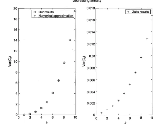
Evidently, now the numbers are approximately 1000 times bigger.

Similarly, Figure 2 depicts the comparison for a decreasing annuity (see Example 2.3). The left panel presents the outcomes obtained by means of numerical approximation and of Corollary 3.4. As in the previous case, the

14 K. Burnecki et a1.

results tally. The graph in the right panel of Figure 2 was plotted using the formula from Theorem 4.5 by Zaks [4]. We can clearly see that the results differ dramatically from the ones presented in the left panel.

Decreasing annuity

+ Numerical approximation

Fig. 2. Comparison of the analytical (+) and numerical (0) results on variance of the final value of

a decreasing annuity-due. The right panel applies to Theorem 4.5 from Zaks [4] and the left one to Corollary 3.4.

Finally, Figure 3 depicts the comparison for an annuity with payments varying in geometric progression with p = 1 and q = 1 +u (see Example 2.5),

where we set tc = 0.1. As before, we can observe in the left panel that our analytical (see Corollary 3.5) and numerical results agree while the correspon- ding Theorem 4.6 from Zaks [4] yields outcome which is essentially smaller (right panel). It is even negative for k = 1.

We conducted similar tests for general annuities with payments varying in arithmetic and geometric progression (see Theorems 3.1 and 3.2). Since they do not have an equivalence in the paper by Zaks [4], we only compared analytical outcomes with numerical approximations. The results have always, as in the foregoing special cases, coincided.

Annuities under random rates of interest 15 Payments varying in geometric progression

+ Numerical approximation

x 1 0-=

4 I

I

+ Zaks results

I

Fig. 3. Comparison of the analytical (+) and numerical (0) results on variance of the final value of an

annuity-due with payments varying in geometric progression with p = 1 and q = 1 +u. The right panel

applies to Theorem 4.6 from Zaks [4] and the left one to Corollary 3.5. See also Bumecki et al. [I].

REFERENCES

[I] K. B u r n e c ki, A. M a r c i n i u k and A. W e r on, Annuities under random rates of interest - re-

visited, Insurance Math. Econorn. 32 (2003), pp. 457460.

[2] H. U. G e r b e r , L f e Insurance Mathematics, Springer, Berlin 1997.

[3] S. G. Kellison, The Theory of Interest, Irwin, IL, 1991.

141 A. Z a k s, Annuities under random rates of interest, Insurance Math. Econom. 28 (2001), pp. 1-11.

Krzysztof Burnecki and Aleksander Weron Agnieszka Marciniuk Hugo Steinhaus Center for Stochastic Methods Department of Statistics Institute of Mathematics and Economic Cybernetics Wrociaw University of Technology Wrociaw University of Economics 50-370 Wroctaw, Poland 53-345 Wroclaw, Poland E-mail: burnecki@im.pwr.wroc.pl

weron@im.pwr.wroc.pl

E-mail: aga-marciniuk@tlen.pl