Cathy Maugis, Gilles Celeux, Marie-Laure Martin-Magniette
To cite this version:
Cathy Maugis, Gilles Celeux, Marie-Laure Martin-Magniette. Variable selection in model-based
discriminant analysis. [Research Report] RR-7290, INRIA. 2010.
<
inria-00483229
>
HAL Id: inria-00483229
https://hal.inria.fr/inria-00483229
Submitted on 12 May 2010
HAL
is a multi-disciplinary open access
archive for the deposit and dissemination of
sci-entific research documents, whether they are
pub-lished or not.
The documents may come from
teaching and research institutions in France or
abroad, or from public or private research centers.
L’archive ouverte pluridisciplinaire
HAL
, est
destin´
ee au d´
epˆ
ot et `
a la diffusion de documents
scientifiques de niveau recherche, publi´
es ou non,
´
emanant des ´
etablissements d’enseignement et de
recherche fran¸
cais ou ´
etrangers, des laboratoires
publics ou priv´
es.
a p p o r t
d e r e c h e r c h e
0249-6399 ISRN INRIA/RR--7290--FR+ENG Thème COGVariable selection in model-based discriminant
analysis
Cathy Maugis — Gilles Celeux — Marie-Laure Martin-Magniette
N° 7290
Centre de recherche INRIA Saclay – Île-de-France Parc Orsay Université
Cathy Maugis
∗, Gilles Celeux
†, Marie-Laure Martin-Magniette
‡§Th`eme COG — Syst`emes cognitifs ´
Equipe-ProjetSelect
Rapport de recherche n°7290 — May 2010 — 31 pages
Abstract: A general methodology for selecting predictors for Gaussian gener-ative classification models is presented. The problem is regarded as a model se-lection problem. Three different roles for each possible predictor are considered: a variable can be a relevant classification predictor or not, and the irrelevant classification variables can be linearly dependent on a part of the relevant pre-dictors or independent variables. This variable selection model was inspired by the model-based clustering model of Maugis et al. (2009b). A BIC-like model selection criterion is proposed. It is optimized through two embedded forward stepwise variable selection algorithms for classification and linear regression. The model identifiability and the consistency of the variable selection criterion are proved. Numerical experiments on simulated and real data sets illustrate the interest of this variable selection methodology. In particular, it is shown that this well ground variable selection model can be of great interest to im-prove the classification performance of the quadratic discriminant analysis in a high dimension context.
Key-words: Discriminant, redundant or independent variables, Variable se-lection, Gaussian classification models, Linear regression, BIC
∗Institut de Math´ematiques de Toulouse, INSA de Toulouse, Universit´e de Toulouse †INRIA Saclay - ˆIle-de-France, Projet
select, Universit´e Paris-Sud 11
‡UMR AgroParisTech/INRA MIA 518, Paris
R´esum´e : Nous proposons une m´ethodologie g´en´erale pour la s´election de variables en analyse discriminante par des mod`eles g´en´eratifs gaussiens. Le probl`eme est vu sous un angle de choix de mod`eles. Les variables en comp´etition peuvent avoir trois rˆoles : ce sont soit des pr´edicteurs utiles pour la classification supervis´ee, soit des variables redondantes, li´es aux pr´edicteurs par une r´egression lin´eaire, soit des variables ind´ependantes. Ce mod`ele s’inspire directement du mod`ele de Maugis et al. (2009b) pour la s´election de variables en classification non supervis´ee par des mod`eles de m´elanges de lois gaussiennes. Un crit`ere de type BIC est propos´e pour choisir le rˆole des variables. Ce crit`ere est optimis´e par deux algorithmes emboˆıt´es de s´election ascendante avec remise en cause pour la classification et la r´egression. Nous ´etablissons l’identifiabilit´e de notre mod`ele et nous prouvons l’optimalit´e asymptotique de notre crit`ere. Nous illustrons les bonnes performances de notre approche par des exp´erimentations sur des donn´ees simul´ees et r´eelles. Nous montrons en particulier que notre m´ethodologie de s´election de variables peut ˆetre profitable pour l’analyse discriminante quadratique en grand dimension.
Mots-cl´es : Variables discriminantes, redondantes ou ind´ependantes, S´election de variables, Classification supervis´ee gaussienne, R´egression lin´eaire, BIC
1
Introduction
The task of supervised classification is to build a classifier which enables us to assign an object described by predictors to one of known classes. Such classifiers are built from a training set of objects for which the predictor measurements and the class labels are known. A lot of different methods are available, see for instance the recent books on statistical learning by Hastie et al. (2009) or Bishop (2006). Those methods differ in the way they approach the problem. Generative models, as Linear Discriminant Analysis (LDA) and Quadratic Discriminant Analysis (QDA), estimate the class-conditional densities. The predictive models (for instance logistic regression, classification trees and thek-nearest-neighbor classifier) directly estimate the posterior class probabilities. Non probabilistic methods, as Neural networks and Kernel methods such as Support Vectors, aim at finding the decision function which characterizes the classifier.
Generative models are less parsimonious than predictive and non probabilis-tic methods. Those last methods are generally preferred to generative models when the number of predictors is large in regard to the number of objects in the training set. However, generative models have some advantages since they allow us to determine the marginal density of the data. As noted in Hastie et al. (2009), LDA and QDA are widely used and perform well on an amazingly large and diverse set of classification problems. Moreover LDA is regarded as a reference method by many practitioners, and an advantage of LDA over QDA is that it is a more parsimonious method.
Much efforts have been paid in variable selection for classification, see the reviews of Guyon and Ellisseeff (2003) and Mary-Huard et al. (2007). In this paper, we concentrate our attention on variable selection for Gaussian generative models. There exists quite efficient methods to select predictors in the LDA context. Efficient stepwise variable selection procedures are available in most statistical softwares (see McLachlan, 1992, Section 12.3.3). On the contrary, there is less available material for QDA (Young and Odell, 1986), and as far as we know, no variable selection procedure for QDA is available in standard statistical softwares. However in the last few years, there is a renewal of interest in this topic. Zhang and Wang (2008) proposed a variable selection procedure for QDA based on a BIC criterion and Murphy et al. (2010) have adapted the variable selection procedure of Raftery and Dean (2006) to the supervised classification context.
The purpose of this paper is to extend the general variable selection mod-elling proposed in Maugis et al. (2009b), conceived for model-based clustering to the Gaussian classification models. This modelling is the result of successive improvements of variable selection modelling in model-based clustering (Raftery and Dean, 2006; Maugis et al., 2009a,b). Acting in such a way, we dramatically strengthen the appeal of non linear Gaussian classifiers, proposed by Bensmail and Celeux (1996) which are up to now limited by the large number of param-eters to be estimated. The models and variable selection algorithms proposed not only lead to interpret the roles of variables in a clear way, but they also lead to much increase the discriminative efficiency of methods such as QDA.
The paper is organized as follows. In Section 2, Gaussian models of classifi-cation are recalled. Our variable selection approach is presented in Section 3. It makes use of a model which states a clear distinction between useful, redundant and noisy variables for the classification task in the Gaussian framework. It
leads to a BIC-like criterion to be optimized (Section 4). It is proved in Sec-tion 5 that our approach leads to identifiable classificaSec-tion models and that our variable selection criterion is consistent under mild assumptions. In Section 6, a variable selection algorithm using two forward stepwise algorithms is described to determine the roles of the predictors. Applications on simulated and real data sets are presented in Section 7. A short discussion section ends the paper and the proofs of the theorems of Section 5 are postponed to Appendices B and C.
2
Gaussian classification models
Training data for discriminant analysis are composed bynvectors
(x, z) ={(x1, zn), . . . ,(xn, zn); xi ∈RQ, zi∈ {1, . . . , K}},
where xi is the Q-dimensional predictor and zi is the class label of the ith
subject. We assume that the prior probability of the classGk isP(z=k) =pk
with pk > 0 for any k, 1 ≤ k ≤K and P K
k=1pk = 1. The class conditional
density of classGk is modelled with aQ-dimensional Gaussian density: xi|zi=
k ∼ NQ(µk,Σk) where µk ∈ RQ is the mean vector and Σk is the Q×Q
variance matrix. The aim of discriminant analysis is to design a classifier from the training sample, allowing us to estimate the label of any new observation
x∈RQ.
Gaussian generative models differ essentially in their assumptions about the variance matrices. The most commonly applied method, called linear discrimi-nant analysis (LDA), assumes that the variance matrices of the different class are equal. When the variance matrices are totally free, the method is called quadratic discriminant analysis (QDA). Bensmail and Celeux (1996) general-ize the LDA and QDA methods in the Eigenvalue Decomposition Discriminant Analysis (EDDA). As in Banfield and Raftery (1993) and Celeux and Govaert (1995), EDDA is based on the eigenvalue decomposition of the variance matrices
∀k∈ {1, . . . , K}, Σk =LkDkAkD0k
where Lk =|Σk|
1
Q, Dk is the Σk’s eigenvector matrix and Ak is the diagonal
matrix of the normalized eigenvalues of Σk. Those elements respectively
con-trol the volume, the orientation and the shape of the density contour of class
Gk. According to constraints required on the three elements of the eigenvalue
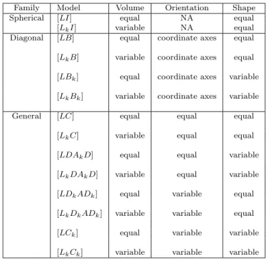
decomposition, a collectionMof 14 more or less parsimonious and easily inter-preted models is available (see Table 4 in Appendix A). Those 14 models are available in themixmodsoftware (Biernacki et al., 2006) and, for most of them, in the mclust software (Fraley and Raftery, 2003). The LDA and QDA are implemented in several softwares as well as R in the library MASS.
The model selection in the EDDA context consists of choosing the best form of the variance matrices. The best model is usually selected by minimising the cross-validated classification error rate (Bensmail and Celeux, 1996). An-other possible selection criterion is the Bayesian information criterion (Schwarz, 1978) which is an asymptotic approximation of the integrated loglikelihood. The model which maximizes the Bayesian information criterion (BIC) is selected. In this paper a selection by the BIC is considered. Notice that BIC focuses on the
model fit rather than the minimisation of the misclassification rate and is much cheaper to compute.
Once a model of the collection is selected, a new observationx0is assigned to
the group for which its a posteriori probability is maximum. It is theMaximum A Posteriorirule and it is equivalent to find the classk? such that
k?= argmax
1≤k≤K
pkΦ(x|µk,Σk(m)),
where Φ(.|µk,Σk(m)) denotes the Gaussian density with mean vector µk and
variance matrix Σk(m)fulfilling the formm∈ M.
3
The variable selection model collection
Each of theQavailable variables brings information (its own ability to separate the classes), and noise (its sampling variance). Thus it is important to select the variables bringing more discriminant information than noise. In practice there are three kinds of variables: The discriminant variables useful for the classification task, the redundant variables linked to the discriminant variables, and the noisy variables which bring no information for the classification task. Thus, variable selection is an important part of discriminant analysis to get a reliable and parsimonious classifier. Considering the classification problem in the model-based discriminant analysis context allows us to recast variable selection into a model selection problem and to adapt the variable selection model for model-based clustering of Maugis et al. (2009b) in the supervised classification context.
In our modelling, the variables have three possible roles: relevant, redundant or independent for the discriminant analysis. The nonempty set of relevant predictors is denoted as S and the independent variable subset is denoted as
W. The redundant variables, whose the subset is denoted as U, are explained by a variable subset RofS according to a linear regression while the variables in W are assumed to be independent of all the relevant variables. Note that if U is empty, R is empty too and otherwise R is assumed to be not empty. Thus denotingF the family of variable index subsets of{1, . . . , Q}, the variable partition set can be described as follows:
V = (S, R, U, W)∈ F4; S∪U∪W ={1, . . . , Q} S∩U =∅, S∩W =∅, U∩W =∅ S6=∅, R⊆S R=∅ ifU =∅ andR6=∅ otherwise .
Throughout this paper, a quadruplet (S, R, U, W) of V is denoted as V =
(S, R, U, W).
The law of the training sample is modelled by,∀(x, z)∈RQ× {1, . . . , K},
f(x|z=k, m, r, l,V) = Φ(xS|µk,Σk(m)) Φ(xU|a+xRβ,Ω(r)) Φ(xW|γ, τ(l)) (1Iz=1, . . . ,1Iz=K) ∼ Multinomial(1;p1, . . . , pK) where
• on the discriminant variable subsetS, the variance matrices Σ1(m), . . . ,ΣK(m)
fulfill the constraints of the formm∈ M(see Section 2);
• on the redundant variable subsetU, the density Φ(xU|a+xRβ,Ω(r))
cor-responds to the linear regression density of xU onxR, where the vector
ais the intercept vector,β is the regression coefficient matrix and Ω(r)is
the variance matrix; this last matrix is assumed to have a spherical ([LI]), diagonal ([LB]) or a general ([LC]) form, and this form is specified by
r∈ Treg={[LI],[LB],[LC]};
• on the independent variable subset W, the marginal density is assumed to be a Gaussian density with meanγ and variance matrixτ(l)which can
be spherical or diagonal and is specified byl∈ Tindep={[LI],[LB]}.
Finally the model collection is
N ={(m, r, l,V);m∈ M, r∈ Treg, l∈ Tindep,V∈ V} (1)
and the likelihood of model (m, r, l,V) is given by
f(x, z|m, r, l,V, θ) = n Y i=1 K Y k=1 pkΦ(xSi|µk,Σk(m)) Φ(xUi |a+x R i β,Ω(r)) Φ(xWi |γ, τ(l)) 1Izi=k
where the parameter vectorθ= (α(m), a, β,Ω(r), γ, τ(l)) with
α(m)= (p1, . . . , pK, µ1, . . . , µK,Σ1(m), . . . ,ΣK(m))
belongs to a parameter vector set Υ(m,r,l,V).
4
Model selection criterion
The model collection N allows us to recast the variable selection problem for Gaussian discriminant analysis into a model selection problem. Ideally, we search the model maximizing the integrated loglikelihood
( ˜m,˜r,˜l,V˜) = argmax (m,r,l,V)∈N ln[f(x, z|m, r, l,V)] where f(x, z|m, r, l,V) = Z f(x, z|m, r, l,V, θ)Π(θ|m, r, l,V)dθ,
Π being the prior distribution of the vector parameter. Since this integrated log-likelihood is difficult to evaluate, it could be approximated by the BIC criterion (Schwarz, 1978). Then the selected model satisfies
( ˆm,r,ˆ ˆl,Vˆ) = argmax
(m,r,l,V)∈N
crit(m, r, l,V) (2)
where the model selection criterion is defined by crit(m, r, l,V) = BICda(x S, z|m) + BIC reg(x U|r,xR) + BIC indep(x W|l), (3) where
• the BIC criterion for the Gaussian discriminant analysis on the relevant variable subsetS is given by
BICda(x S , z|m) = 2 n X i=1 ln "K X k=1 ˆ pkΦ(xSi|µˆk,Σˆk(m))1Izi=k # −λ(m,S)ln(n)
where ˆα(m)is the maximum likelihood estimator andλ(m,S)is the number
of free parameters for the modelmon the variable subsetS.
• the BIC criterion for the linear regression of the variable subset U onR
is defined by BICreg(x U|r,xR) = 2 n X i=1 ln[Φ(xUi |ˆa+xRi β,ˆ Ωˆ(r))]−ν(r,U,R)ln(n) (4)
where ˆa, ˆβ and ˆΩ(r) are the maximum likelihood estimators andν(r,U,R)
is the number of free parameters of the linear regression.
• the BIC criterion associated to the Gaussian density on the variable subset
W is given by BICindep(x W |l) = 2 n X i=1 ln[Φ(xWi |γ,ˆ ˆτ(l))]−ρ(l,W)ln(n).
The parameters ˆγand ˆτ(l)denote the maximum likelihood estimators and
ρ(l,W) is the number of free parameters of the Gaussian density.
• the maximum likelihood estimator is denoted as ˆθ= ( ˆα(m),ˆa,β,ˆ Ωˆ(r),ˆγ,τˆ(l))
and the overall number of free parameters is Ξ(m,r,l,V)=λ(m,S)+ν(r,U,R)+
ρ(l,W).
5
Theoretical properties
The theoretical properties established in Maugis et al. (2009b) in the model-based clustering framework can be adapted to the Gaussian discriminant anal-ysis context. First, necessary and sufficient conditions are given to ensure the identifiability of the model collection. Second, a consistency theorem of the model selection criterion is stated.
5.1
Identifiability
In order to ensure the model identifiability, some natural conditions are required to distinguish the discriminant density part to the regression and the indepen-dent Gaussian density parts. For instance, if s is a non empty subset strictly included into the relevant variable subsetS and ¯sis its complement inS then the identifiability cannot be ensured if the regression density of ¯son scan be regrouped with the regression density of U on R. Despite the fact that Con-ditions (C1)-(C3) of Theorem 1 look rather technical, they are quite natural and Theorem 1 is saying that our variable selection model is identifiable in all situations of interest.
The following additional notation is introduced to state the model identi-fiability theorem. Recall that Φ(.|µk,Σk) denotes the Gaussian density with
mean µk and variance matrix Σk. The parameters can be decomposed into
µk = (µks, µk¯s) and Σk into submatrices Σk,ss, Σk,s¯s and Σk,¯ss¯, wheres is a
nonempty subset of S and ¯s its complement in S. Moreover, conditional pa-rameters are defined byµk,s|s¯ =µk¯s−µksΣ−k,ss1 Σk,ss¯, Σk,¯s|s = Σ−k,ss1 Σk,s¯s and
Σk,¯ss|s¯ = Σk,¯ss¯−Σk,ss¯ Σ−k,ss1 Σk,ss¯. For two subsetssandt, the following
restric-tions of aI×J matrix Λ are considered: Λst= (Λij)i∈s,j∈t, Λ.t= (Λij)1≤i≤I,j∈t
and Λs.= (Λij)i∈s,1≤j≤J.
Theorem 1. LetΘ(m,r,l,V)be a subset of the parameter setΥ(m,r,l,V)such that elementsθ= (α, a, β,Ω, γ, τ)
(C1) : contain couples (µk,Σk)fulfilling∀s(S,∃(k, k0),1≤k < k0≤K
µk,s|s¯ 6=µk0,¯s|s orΣk,s|s¯ 6= Σk0,¯s|s orΣk,¯ss|s¯ 6= Σk0,¯s¯s|s,
wheres¯denotes the complement inS of any nonempty subsets ofS.
(C2) : if U 6=∅,
∗ for all variables j of R, there exists a variableu of U such that the restriction βuj of the regression coefficient matrix β associated with
j anduis not equal to zero.
∗ for all variables u of U, there exists a variable j of R such that
βuj 6= 0.
(C3) : Parameters Ω andτ strictly respect the forms r andl respectively: They are both diagonal matrices with at least two different eigenvalues if r = [LB] and l= [LB] and Ωhas at least a non-zero entry outside the main diagonal ifr= [LC].
Let (m, r, l,V) and(m?, r?, l?,V?)be two models. If there exist θ∈Θ
(m,r,l,V)
andθ?∈Θ
(m?,r?,l?,V?) such that
f(.|m, r, l,V, θ) =f(.|m?, r?, l?,V?, θ?)
then(m, r, l,V) = (m?, r?, l?,V?)andθ=θ?.
The complete proof of Theorem 1 is postponed to Appendix B.
5.2
Consistency
A consistency property of our criterion can be checked. In this section, it is proved that the probability of selecting the true model by maximizing Criterion (3) approaches 1 as n → ∞. Denoting h the density function of the sample (x, z), the two following vectors are considered
θ(?m,r,l,V) = argmin θ(m,r,l,V)∈Θ(m,r,l,V) KL[h, f(.|m, r, l,V, θ)] = argmax θ(m,r,l,V)∈Θ(m,r,l,V) E{lnf(X, Z|m, r, l,V, θ)},
where KL[h, f] =R
lnnfh((xx))oh(x)dxis the Kullback-Leibler divergence between the densitieshandf and
ˆ θ(m,r,l,V)= argmax θ(m,r,l,V)∈Θ(m,r,l,V) 1 n n X i=1 ln{f(xi, zi|m, r, l,V, θ)}.
Recall that Θ(m,r,l,V)’s are the subsets defined in Theorem 1 for ensuring the
model identifiability.
The following assumption is considered:
(H1) The density his assumed to be one of the densities in competition. By identifiability, there exists a unique model (m0, r0, l0,V0) and an
associ-ated parameterθ? such thath=f(.|m
0, r0, l0,V0, θ?).
Moreover, an additional technical assumption is considered:
(H2) For all models (m, r, l,V)∈ N, the vectorsθ?and ˆθare supposed to belong
to a compact subspace Θ0(m,r,l,V)in the intersection between Θ(m,r,l,V)and
PK−1(ρ)× B(η,card(S))K× DKcard(S)× B(η,card(U))
×B(η,card(R),card(U))× Dcard(U)× B(η,card(W))× Dcard(W)
! where • PK−1(ρ) = (p1, . . . , pK)∈[ρ,1]K; K P k=1 pk = 1 whereρ >0,
• B(η, r) is the closed ball in Rr of radius η centered at zero for the
l2-norm defined bykxk= s r P i=1 x2 i,∀x∈Rr,
• B(η, r, q) is the closed ball inMr×q(R) of radiusη centered at zero
for the matricial norm|||.|||defined by
∀A∈ Mr×q(R),|||A|||= sup
kxk=1
kxAk,
• Dr is the set of ther×rpositive definite matrices with eigenvalues
in [sm, sM] with 0< sm< sM.
Theorem 2. Under assumptions (H1) and (H2), the model ( ˆm,r,ˆ ˆl,Vˆ) maxi-mizing Criterion (3) is such that
P(( ˆm,r,ˆ ˆl,Vˆ) = (m0, r0, l0,V0)) →
n→∞1.
The proof of this theorem is given in Appendix C.
6
The variable selection procedure
Theorem 2 is reassuring about the theoretical behavior of the model selection Criterion (3). Unfortunately, the number of models given by (1) being huge, an exhaustive search for the model maximizing Criterion (3) is impossible. Thus we design a procedure, embedding forward stepwise algorithms, to determine the best variable roles and the best variance matrix forms.
6.1
The models in competition
At a fixed step of the algorithm, the variable set{1, . . . , Q} is divided into the subset of selected discriminant variablesS, the subsetU of redundant variables which are linked to some discriminant variables, the subsetW of independent irrelevant variables andj the candidate variable for inclusion into or exclusion from the discriminant variable subset. Under the model (m, r, l), the integrated likelihood can be decomposed as
f(xS,xj,xU,xW, z|m, r, l) = f(xU,xW|xS,xj, z, m, r, l)f(xS,xj, z|m, r, l)
= findep(x
W|l)f
reg(x
U|r,xS,xj)f(xS,xj, z|m, r, l)
where findep(xW|l) is the integrated likelihood on the independent irrelevant
variable subsetW andfreg(xU|r,xS,xj) corresponds to the integrated likelihood on the subsetU regressed on variable subset S and the candidate variable j. The expression of the integrated likelihood restricted onS∪ {j}depends on the three situations which can occur for the candidate variablej:
• First situation: GivenxS,xj provides additional information for the dis-criminant analysis thus
f(xS,xj, z|m, r, l) =fda(x
S,xj, z|m)
corresponds to the integrated likelihood for the discriminant analysis on variable subsetS∪ {j}.
• Second situation: Given xS, xj does not provide additional information for the discriminant analysis but has a linear link with a nonempty subset denoted R[j] of S containing the relevant variables for the regression of
xj onxS:
f(xS,xj, z|m, r, l) =fda(xS, z|m)freg(xj|[LI],xR[j]).
The second term in the right-hand side corresponds to the integrated likelihood of the regression ofxj onxR[j]. Sincej is a single variable, the
variance matrix is spherical ([LI]).
• Third situation: GivenxS,xj does not provide additional information for
the discriminant analysis and is independent of all the variables ofS:
f(xS,xj, z|m, r, l) =fda(xS|m)findep(xj|[LI]).
The second term in the right-hand side corresponds to the integrated likelihood of the independent Gaussian density on the variable j with a spherical variance matrix sincej is a single variable.
In order to compare those three situations in an efficient way, we remark thatfindep(x
j|[LI]) can be writtenf
reg(x
j|[LI],x∅). Thus instead of considering
the nonempty subsetR[j] we consider a new explicative variable subset denoted ˜
R[j] and defined by ˜R[j] =∅ ifj follows the third situation and ˜R[j] =R[j] if
j follows the second situation. This allows us to recast the comparison of the three situations into the comparison of two situations with the Bayes factor
fda(xS,xj, z|m)
fda(xS, z|m)freg(xj|[LI],x
˜
This Bayes factor being difficult to evaluate, it is approximated by BICdiff(j|m) = BICda(x
S ,xj, z|m)−nBICda(x S , z|m) + BICreg(x j |[LI],xR˜[j])o. (5)
6.2
The general steps of the algorithm
First, this algorithm consists of separating variables into relevant and irrele-vant variables for the discriminant analysis via a forward stepwise algorithm described in Section 6.3. Second, the irrelevant variables are partitioned into redundant variables, if regressors are chosen inside the relevant variables, and independent variables otherwise. It remains then to determine the set of re-gressors from the relevant variables for the multidimensional regression of the redundant variables and the general variance structures.
I For each mixture formm:
• The variable partition into relevant and irrelevant variables for the discriminant analysis, ˆS(m) and ˆSc(m) respectively, is determined by the forward stepwise selection algorithm described hereafter (see Section 6.3).
• The variable subset ˆSc(m) is divided into ˆU(m) and ˆW(m): For
each variable jbelonging to ˆSc(m), the variable subset ˜R[j] of ˆS(m)
allowing to explain j by a linear regression is determined with the forward stepwise regression algorithm (see Appendix D). If ˜R[j] =∅,
j ∈Wˆ(m) and otherwise,j ∈Uˆ(m).
• For each formr:
∗ The variable subset ˆR(m, r), included into ˆS(m) and explaining the variables of ˆU(m), is determined using the forward stepwise regression algorithm with the fixed form regression modelr(see Appendix D).
∗ For each forml: ˆθand the following criterion value are computed
g
crit(m, r, l) = crit(m, r, l,Sˆ(m),Rˆ(m, r),Uˆ(m),Wˆ(m)).
I The model satisfying the following condition is then selected ( ˆm,ˆr,ˆl) = argmax
(m,r,l)∈M×Treg×Tindep
g
crit(m, r, l).
I Finally, the complete selected model is
ˆ
m,ˆr,ˆl,Sˆ( ˆm),Rˆ( ˆm,rˆ),Uˆ( ˆm),Wˆ( ˆm).
Our variable selection procedure is based on forward stepwise algorithms which allow to study data sets where the individual number nis smaller than the variable numberQ. Nevertheless, for studying a data set where Q≤n, a backward procedure (starting the search with all variables) could be preferred because it takes variable interactions into account.
6.3
The forward stepwise selection algorithm
InitialisationLetmfixed, S(m) =∅,Sc(m) ={1, . . . , Q},jI =∅ andjE=∅.
The algorithm is making use of an inclusion and an exclusion steps now de-scribed. The decision of including (resp. excluding) a variable in (resp. from) the discriminant variable subset is based on (5). Starting from a preliminary inclusion step, the forward variable selection algorithm consists of alternating inclusion and exclusion steps. It returns the discriminant variable subset ˆS(m) and the irrelevant variable subset ˆSc(m). These different steps are now
de-scribed.
Preliminary inclusion stepThis step consists of selecting the first discrimi-nant variable. For allj inSc(m), compute
BICdiff(j|m) = BICda(x
j, z|m)−BIC reg(x j|[LI],x∅) and determine jI = argmax j∈Sc(m) BICdiff(j|m).
ThenS(m) ={jI},Sc(m) =Sc(m)\{jI} and go to the inclusion step.
Inclusion step For all j in Sc(m), use the forward stepwise regression al-gorithm (see Appendix D) to determine the subset ˜R[j] for the regression ofxj
onxS(m). And, compute
BICdiff(j|m) = BICda(x
S(m),xj, z|m)−nBIC da(x S, z|m) + BIC reg(x j|[LI],xR˜[j])o. Then, compute jI = argmax j∈Sc(m) BICdiff(j|m).
• If BICdiff(jI|m)>0, S(m) = S(m)∪ {jI}, Sc(m) = Sc(m)\{jI} and, if
jI 6=jE, go to the exclusion step and stop otherwise.
• Otherwise,jI =∅. IfjE6=∅, go to the exclusion step and stop otherwise.
Exclusion step For all j in S(m), use the forward stepwise regression algo-rithm (see Appendix D) to determine the subset ˜R[j] for the regression of xj
onxS(m)\j. And, compute
BICdiff(j|m) = BICda(x
S(m), z|m)−nBIC da(x S(m)\{j}, z|m) + BIC reg(x j|[LI],xR˜[j])o. Then, compute jE= argmin j∈S(m) BICdiff(j|m). • If BICdiff(jI|m) < 0, S c(m) = Sc(m)∪ {j E}, S(m) = S(m)\{jE}. If
jE6=jI, go to the inclusion step and stop otherwise.
7
Applications
We present numerical experiments to assess our variable selection procedure. First, the interest of variable selection for non linear discriminant analysis mod-els such as QDA is highlighted on simulated data. Then, two applications on real data sets are presented. The application on the Landsat Satellite data set allows us to illustrate the interest of precising the role of the variables in an explicative perspective and again the great interest of our variable selection procedure to improve the classification performances of QDA. The second application con-cerns the Leukemia data of Golub et al. (1999), a classical genomics example where the number of variables is greater than the number of observations.
7.1
Simulated example
This simulated example consists of considering samples described by Q = 16 variables. The prior probabilities of the four classes are assumed to bep1= 0.15,
p2 = 0.3, p3 = 0.2 and p4 = 0.35. On the three discriminant variables, data
are distributed fromx{i1−3}|zi=k∼Φ(.|µk,Σk) withµ1= (1.5,−1.5,1.5), µ2=
(−1.5,1.5,1.5), µ3= (1.5,−1.5,−1.5), µ4= (−1.5,1.5,−1.5), and Σk =
ρ|i−j|k
1≤i,j≤3
withρ1= 0.85, ρ2= 0.1, ρ3= 0.65 andρ4= 0.5. Four redundant variables
sim-ulated from x{i4−7}∼ N x{i1,3} 1 0 −1 2 0 −2 2 1 ;I4
and nine independent variables are appended, sampled fromx{i8−16}∼ N(γ, τ) with
γ= (−2,−1.5,−1,−0.5,0,0.5,1,1.5,2)
and
τ= diag(0.5,0.75,1,1.25,1.5,1.25,1,0.75,0.5).
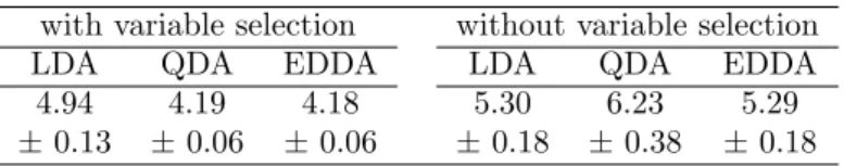
A total of 100 simulation replications are considered where the training sample is composed of n = 500 data points and the same test sample with 50,000 points is used. The LDA, QDA and EDDA methods with and without variable selection are compared according to the averaged classification error rates.
Results summarized in Table 1 show that the variable selection procedure allows to improve the classification performance of LDA, QDA and EDDA. In particular, QDA becomes superior to LDA with variable selection. In all replications, only the first three variables are declared discriminant. When the true variable partition is not selected, it is due to some independent variables which are declared redundant (24, 24 and 26 times for EDDA, QDA and LDA respectively).
with variable selection without variable selection
LDA QDA EDDA LDA QDA EDDA
4.94 4.19 4.18 5.30 6.23 5.29
±0.13 ±0.06 ±0.06 ±0.18 ±0.38 ±0.18
Table 1: Averaged classification error rate (± standard deviation) for LDA, QDA and EDDA methods, with and without variable selection for the simulated data sets.
7.2
The Landsat Satellite Data
The Landsat Satellite Data, available at the UCI Machine Learning Repository
(seehttp://www.ics.uci.edu/~mlearn/) is considered. This data set consists
of the multi-spectral values of pixels in a tiny sub-area of a satellite image. Each line is a vector of lengthQ= 36, composed of the pixel values in four spectral bands (two in the visible region and two in the near infra-red) of each of the 9 pixels in the 3×3 neighborhood. These data points are split into six classes. The original data set has already been divided into a training set with 4,435 samples and a testing set with 2,000 samples. The same experiment conditions than in Zhang and Wang (2008) are considered: 1,000 samples (randomly selected from the training data) are used to estimate and select the model, and this experiment is randomly replicated 100 times. Only QDA and LDA are considered in this study.
According to Table 2, QDA and LDA perform the same without variable se-lection, while QDA outperforms LDA with variable selection. In all replications, our variable selection procedure selects the QDA model ( ˆm= [LkCk]), and all
the irrelevant classification variables are redundant ( ˆW =∅) and regressed on all discriminant variables ( ˆR = ˆS) with a general covariance matrix structure (ˆr= [LC]).
with variable selection without variable selection
LDA QDA LDA QDA
21.00 16.21 18.05 17.90
±0.53 ±0.68 ±0.48 ±0.57
Table 2: Averaged classification error rate (±standard deviation) for LDA and QDA methods, without and with variable selection for the Landsat Satellite Data.
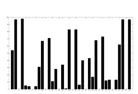
It is noteworthy that QDA and LDA select the same variables in the 100 replications, with an average selection of 12 discriminant variables as in Zhang and Wang (2008). It is worth mentioning some variable selection tendencies (see Figure 1). First, variables tend to be selected by couple: for instance Variables 34 and 36, Variables 18 and 20, and Variables 2 and 4 are both declared discriminant in the same replications. Second, we can note that Variables 3, 7, 11, 15, 19, 23, 27, 31 and 35, corresponding to one measure in the near infra-red for each pixel of the 3×3 neighborhood are never declared discriminant. Third, the variables corresponding to Pixels 1, 3, 5, 7 and 9 in the 3×3 neighborhood are more often declared discriminant than the one of the other pixels, certainly because these pixels have more neighbor pixels in common.
Figure 1: Number of times each variable is declared discriminant among 100 replications for the Landsat Satellite Data.
7.3
Leukemia data set
These data come from a study of gene expression in two types of acute leukemias: acute lymphoblastic leukemia (ALL) and acute myeloid leukemia (AML) pub-lished by Golub et al. (1999). Gene expression levels were measured for 47 ALL tumor samples and 25 AML tumor samples, using Affymetrix high-density oligonucleotide arrays containing 6817 human genes. After the pre-processing steps, as image analysis, standardization and some gene filtering, Q = 3571 genes are conserved. The interest of this data set is the large number of genes describing the samples, and the importance to detect the genes whose expres-sion pattern separate the two types of leukemias. This data set is known as a benchmark data set and numerous results are available (Golub et al., 1999; Su et al., 2003; Krishnapuram et al., 2004; Mary-Huard and Robin, 2009; Yang and Xin-Yuan, 2010). It is considered from two points of view in this section. First, the relevance and stability of our variable selection procedure are measured us-ing a leave-one-out procedure for LDA and QDA models. Second, the interest of variable selection to improve the prediction accuracy is assessed using the training and test samples used by Golub et al. (1999).
In the leave-one-out procedure for LDA and QDA, the averaged classification error rate is equal to zero and so as good as the error rates of different methods already applied (see Mary-Huard and Robin, 2009). For LDA, 3529 genes are never declared discriminant for the classification by our variable selection pro-cedure and 44 of them are always declared independent. Among the 42 genes declared at least once discriminant, seven genes (Macmarcks, CD33 antigen, CST3, DF D, CCND3, GLUTATHIONE S-TRANSFERASE and RABAPTIN-5 protein) are already known to be discriminant and three (PLZF, Adrenal-Specific Protein Pg2 and, PRSS1) are known to be implicated in cancers. The first two genes declared the most time relevant are DF D (67 times) and GLU-TATHIONE S-TRANSFERASE (53 times); the other ones are more declared redundant than relevant. We also compare our results with the list of Su et al.
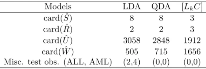
(2003) which contains 100 genes reported as discriminant by at least one dis-criminant method. A lack of precision in the gene names leads to consider 88 genes among these 100 genes. According to our method, 83 genes are mainly declared redundant and six of them (Macmarcks, CD33 antigen, CST3, DF D (adipsin), CCND3 and GLUTATHIONE S-TRANSFERASE) at least once rel-evant. The five remaining genes are declared at least once independent (W) and never discriminant for the classification. Among these five genes, three are very often in W (more than 52 times) but are identified in the Su list by only the t-test procedure. They may be false candidats. The two others (Lamp2 and GLYCYLPEPTIDE TETRADECANOYLTRANSFERASE) are declared redundant 67 and 60 times and otherwise independent. Their status is thus more redundant than independent and it is coherent with their presence in the Su list. We do not report in detail the results in QDA which are quite analo-gous. But it is worthwhile to remark that the number of discriminant variables selected at least one time is 122 for QDA instead of 32 for LDA. It indicates a greater stability of the variable selection procedure for the simpler model LDA. We then analyze the Leukemia data set using 38 (27 are ALL and 11 are AML) samples in the training and 34 (20 are ALL and 14 are AML) samples in the test. Results of our method are given in Table 3 and are compared with the performance of other methods given in Yang and Xin-Yuan (2010). Despite the variable selection, LDA performs poorly, on the contrary the quadratic methods (QDA and [LkC]) are greatly improved by variable selection leading
to zero misclassified test observation. Moreover, this is achieved with a small number of discriminant variables especially for the parsimonious model [LkC]
(see Appendix A).
Models LDA QDA [LkC]
card( ˆS) 8 8 3
card( ˆR) 2 2 3
card( ˆU) 3058 2848 1912 card( ˆW) 505 715 1656 Misc. test obs. (ALL, AML) (2,4) (0,0) (0,0)
Table 3: Variable selection and misclassification error rate. The first four lines indicate the number of variables inS,R,U andW sets. The last line gives the number of misclassified test observations according to the two leukemia types ALL and AML.
8
Discussion
We have proposed a variable selection methodology for a large family of Gaus-sian generative models in discriminant analysis. Regarding the problem as a model selection problem, we have proposed a BIC-like criterion to distinguish between discriminant, redundant and noisy variables. We proved the identi-fiability of our model collection and the consistency of the proposed BIC-like criterion. A procedure embedding two forward stepwise variable selection al-gorithms for classification and regression has been defined. Numerical experi-ments highlight the potentially great interest of our variable selection procedure to improve the classification performances of non linear Gaussian classification
models. Actually those models involve many parameters when the number of variables is large with respect to the training sample size. But our variable selection procedure allows us to overcome the dimensionality problem leading to powerful classifiers with a nice interpretation of variable roles. Those re-sults confirm the promising performances obtained by Murphy et al. (2010) and Zhang and Wang (2008) with less general methods. Our opinion is that our methodology is able to make the non linear generative classification methods such as quadratic discriminant analysis much more efficient in high dimensional contexts and competitive with gold standard classifiers such as LDA, logistic regression, k-nearest neighbor classifier or support vector classifiers in many situations.
Appendices
A
The different model forms
This is the list of the 14 different model forms available in themixmodsoftware.
Family Model Volume Orientation Shape Spherical [LI] equal NA equal [LkI] variable NA equal Diagonal [LB] equal coordinate axes equal [LkB] variable coordinate axes equal [LBk] equal coordinate axes variable [LkBk] variable coordinate axes variable General [LC] equal equal equal
[LkC] variable equal equal [LDAkD] equal equal variable [LkDAkD] variable equal variable [LDkADk] equal variable equal [LkDkADk] variable variable equal [LCk] equal variable variable [LkCk] variable variable variable Table 4: List of model forms available in mixmod.
B
Proof of the model identifiability
Theorem1 concerning the model identifiability can be proved quickly (see Proof 1) using the SRUW model identifiability established in Maugis et al. (2009b) in the model-based clustering context. It is also possible to completely prove this theorem in the discriminant analysis context (see Proof 2).
Proof 1. Let (m, r, l,V)and(m?, r?, l?,V?)be two models. Letθ∈Θ
(m,r,l,V)
and θ? ∈ Θ
(m?,r?,l?,V?) two parameters vectors such that ∀x ∈ RQ, ∀z ∈
{1, . . . , K},
f(x, z|m, r, l,V, θ) =f(x, z|m?, r?, l?,V?, θ?).
It is equivalent to the following system: ∀x∈RQ, ∀k∈ {1, . . . , K},
pkΦ(xS|µk,Σk(m)) Φ(xU|a+xRβ,Ω(r)) Φ(xW|γ, τ(l)) = p?kΦ(xS|µ?k,Σ ? k(m?)) Φ(x U |a?+xRβ?,Ω?(r?)) Φ(x W |γ?, τ(?l?)) (6)
Summing theK previous equations, we obtain that n PK k=1pkΦ(xS|µk,Σk(m)) o Φ(xU|a+xRβ,Ω (r)) Φ(xW|γ, τ(l)) =nPK k=1p ? kΦ(x S|µ? k,Σ ? k(m?)) o Φ(xU|a?+xRβ?,Ω? (r?)) Φ(xW|γ?, τ(?l?)).
Next, using the identifiability result established in Maugis et al. (2009b) in the clustering framework with a fix number of components K, we obtain that m=
m?, r =r?, l =l?, a =a?, β =β?, Ω
(r) = Ω?(r?) and the parameters pk, p?k,
µk,µ?k and Σ?k(m),Σ
?
k(m?) are equal up to a permutation of Gaussian mixture
components. But this permutation is the identity according to (6) thus pk =p?k,
µk =µ?k andΣ
?
k(m)= Σ
?
k(m?) for allk∈ {1, . . . , K}.
Proof 2. Let (m, r, l,V)and(m?, r?, l?,V?)be two models. Let θ∈Θ
(m,r,l,V)
and θ? ∈ Θ
(m?,r?,l?,V?) two parameters vectors such that ∀x ∈ RQ, ∀z ∈
{1, . . . , K},
f(x, z|m, r, l,V, θ) =f(x, z|m?, r?, l?,V?, θ?).
It is equivalent to the following system: ∀x∈RQ, ∀k∈ {1, . . . , K},
pkΦ(xS|µk,Σk(m)) Φ(xU|a+xRβ,Ω(r)) Φ(xW|γ, τ(l))
= p?kΦ(xS|µ?
k,Σ
?
k(m?)) Φ(xU|a?+xRβ?,Ω?(r?)) Φ(xW|γ?, τ(?l?))
and can be reformulated as
pkΦ(x|Ak, Bk) =p?kΦ(x|A
?
k, B
?
k) (7)
where the Q-dimensional vectorsAk are defined by
∀j∈ {1, . . . , Q}, Akj=
µkj if j∈S
(d+µkΛ)j if j∈Sc
and theQ×Q-dimensional matrices Bk are defined by
∀(i, j)∈ {1, . . . , Q}2, B k,ij = Σk(m),ij ifi∈S, j∈S (Σk(m)Λ)ij ifi∈S, j∈Sc (Λ0Σk(m))ij ifi∈Sc, j∈S (D+ Λ0Σk(m)Λ)ij ifi∈Sc, j∈Sc with ∀j∈Sc, dj = aj if j∈U γj if j∈W ∀j∈Sc, ∀h∈S, Λjh= βjh if j∈U, h∈R 0 otherwise and ∀(i, j)∈(Sc)2, Dij = Ω(r),ij if i∈U, j∈U τ(l),ij if i∈W, j ∈W 0 otherwise.
In the same way, we define theA?k’s andB?k’s. In order to make easier the reading of this proof, the indexation ofΣk,Ωandτ bym,r andl are omitted.
First according to (7), for all k∈ {1, . . . , K}, pk =pk?, Ak =A?k andBk =
B?
k. Indeed if there exists k such that pk < p?k then ∀x∈ RQ, Φ(x|Ak, Bk) >
Φ(x|A?
k, Bk?) and that is in contradiction with the fact that Φ(.|Ak, Bk) and
Φ(.|A?
k, Bk?)are two densities.
Second, assume that S∩S? =∅ and consider the subsetss=S?∩Sc and
t=S? c∩S. The equality of variance matricesBk andBk? on sand between s
andtgives respectively for allk∈ {1, . . . , K},
Dss+ Λ0.sΣkΛ.s= Σ?k
Λ0.sΣk = Σ?kΛ?.t
.
According to these two equalities, it is deduced thatDss= Σ?k(I−Λ?.tΛ.s)for all
k. SinceDss andΣ?k are positive definite matrices,I−Λ?.tΛ.s is a nonsingular
matrix and consequently all the variance matrices Σ?
k =Dss(I−Λ?.tΛ.s)−1 are
equal. Moreover, the equality of mean vectors ons andtgives
ds+µkΛ.s=µ?k µk =d?t+µ?kΛ ? .t , implying thatµ? k(I−Λ ?
.tΛ.s) =ds+d?tΛ.s, for all k. SinceI−Λ?.tΛ.s is
nonsin-gular, allµ?
k are equal. This is in contradiction with the assumption (C1).
Third, assume thatS∩S?6=∅andSc∩S? c6=∅, and consider the nonempty
subsets t = Sc∩S?, s =S ∩S? and s¯= S∩S? c. The equality of variance
matricesBk andBk? ons¯, ons, between t ands, betweensands¯, and between
tands¯gives respectively for allk,
Σk,s¯s¯ = Ds?¯¯s+ Λ ?0 s¯s(Σ ? k,ssΛ ? s¯s+ Σ ? k,stΛ ? ts¯) + Λ ?0 t¯s(Σ ? k,tsΛ ? s¯s+ Σ ? k,ttΛ ? t¯s) (8) Σk,ss = Σ?k,ss (9) Λ0st¯Σk,¯ss+ Λ0stΣk,ss = Σ?k,ts (10) Σk,ss¯ = Λ? 0 s¯sΣ ? k,ss+ Λ ?0 ts¯Σ ? k,ts (11) Σk,¯ss¯Λst¯ + Σk,ss¯Λst = Λ? 0 s¯sΣ ? k,st+ Λ ?0 ts¯Σ ? k,tt . (12) From (8), (11), (12), we get Σk,¯ss¯(I−Λ¯stΛ?t¯s) =D ? ¯ s¯s+ Σk,ss¯(Λ?ss¯+ Λ ? stΛts¯) (13)
and Equations (9), (10) and (11) allow to deduce
Λ?s¯s+ Λ?stΛt¯s= Σ−k,ss1 Σk,ss¯(I−Λst¯Λ?t¯s). (14)
Finally, Equations (13) and (14) imply Σk,s¯s|s¯ (I−Λst¯Λ?ts¯) = D?¯ss¯. Since Ds?¯¯s
andΣk,¯s¯s|s are positive definite matrices, the matrixI−Λ¯stΛ?t¯s is nonsingular
and all the matricesΣk,s¯¯s|sare equal. Similarly, according to (14), all matrices
Σk,¯s|s are equal. The equality of mean vectors ons¯,s andt gives the following
equations: For allk,
µks¯=d?s¯+µ?ksΛ?ss¯+µ?k,tΛ?ts¯ µks=µ?ks dt+µk¯sΛst¯ +µksΛst=µ?k,t implying µks¯(I−Λ¯stΛ?ts¯) = (d ? ¯ s+dtΛ?ts¯) +µks(Λ?ss¯+ ΛstΛ?ts¯)
and Equation (14) leads to
(µk¯s−µksΣk,ss−1 Σk,s¯s)(I−Λst¯Λ?t¯s) =d¯s+d?tΛ ? t¯s .
Since I−Λst¯Λt?s¯ is non singular, the mean vectors µk,s|s¯ are also equal, and thus the constraint (C1) is violated. In the same way, assuming that s¯or t is empty, we prove that S(S? andS?(S are impossible.
Finally, it leads to S = S? and, by the equality of variance matrices and mean vectors, we easily obtain that µk = µ?k, Σk = Σ?k (and then m = m
?),
d =d?, D =D? and Λ = Λ?. ThenR =R? because otherwise, according to
the definition of Λ, there exists h ∈ R∩R? c such that ∀u ∈ U, β
hu = 0 or
there exists h ∈ R?∩Rc such that ∀u ∈ U?, β?
hu = 0 that is contradicted the
assumption (C2). In same way, we prove that U = U? and thus W = W?.
Finally, according to the definition of Λ, d and D, we obtain that β = β?,
Ω = Ω?,r=r?,a=a?,γ=γ?,τ=τ? andl=l?.
C
Proof of the criterion consistency theorem
This appendix is devoted to the proof of Theorem 2 given the criterion consis-tency.
Proof. According to the expressions (2) and (3), the selected model satisfies ( ˆm,ˆr,ˆl,Vˆ) = argmax (m,r,l,V)∈N crit(m, r, l,V) with crit(m, r, l,V) = 2 n X i=1 ln[f(xi, zi|m, r, l,V,θˆ)]−Ξ(m,r,l,V)ln(n). Thus P(( ˆm,r,ˆ ˆl,Vˆ) = (m0, r0, l0,V0)) =P(crit(m0, r0, l0,V0)−crit(m, r, l,V)≥0,∀(m, r, l,V)∈ N). (15)
Denoting ∆crit(m, r, l,V) = crit(m0, r0, l0,V0)−crit(m, r, l,V), we get
∆crit(m, r, l,V) = 2n " 1 n n X i=1 ln ( f(xi, zi|m0, r0, l0,V0,θˆ) h(xi, zi) ) −1 n n X i=1 ln ( f(xi, zi|m, r, l,V,θˆ) h(xi, zi) )# + Ξ(m,r,l,V)−Ξ(m0,r0,l0,V0) ln(n). (16)
LetN1 ={(m, r, l,V)∈ N; KL[h, f(.|m, r, l,V, θ?)]6= 0}. We have thatN1=
N \{(m0, r0, l0,V0)}since if KL[h, f(.|m, r, l,V, θ?)] = 0 thenh=f(.|m0, r0, l0,V0, θ?) =
f(.|m, r, l,V, θ?) and according to the model identifiability, (m
0, r0, l0,V0) =
(m, r, l,V). Thus from (15), the theorem is established if it is proved that
∀(m, r, l,V)∈ N1, P(∆crit(m, r, l,V)<0) →
Let (m, r, l,V) ∈ N1. Denoting Mn(m, r, l,V) = n1 n P i=1 lnnf(xi,zi|m,r,l,V,θˆ) h(xi,zi) o
andM(m, r, l,V) =−KL[h, f(.|m, r, l,V, θ?)], from (16) we have
P(∆crit(m, r, l,V)<0) = P(2n{Mn(m0, r0, l0,V0)−Mn(m, r, l,V)} +Ξ(m,r,l,V)−Ξ(m0,r0,l0,V0) ln(n)<0) = P(Mn(m0, r0, l0,V0)−M(m0, r0, l0,V0) +M(m, r, l,V)−Mn(m, r, l,V) +M(m0, r0, l0,V0)−M(m, r, l,V) + Ξ(m,r,l,V)−Ξ(m0,r0,l0,V0) ln(n) 2n <0 ! .
Thus, for all >0, according to Lemma 7,
P(∆crit(m, r, l,V)<0) ≤ P(M(m0, r0, l0,V0)−Mn(m0, r0, l0,V0)> ) +P(Mn(m, r, l,V)−M(m, r, l,V)> ) +P M(m0, r0, l0,V0)−M(m, r, l,V) + Ξ(m,r,l,V)−Ξ(m0,r0,l0,V0) ln(n) 2n <2 ! .
From Lemma 3, stated hereafter,∀(m, r, l,V)∈ N,Mn(m, r, l,V) P → n→∞M(m, r, l,V). Thus, ∀ >0, P(Mn(m, r, l,V)−M(m, r, l,V)> )≤P(|Mn(m, r, l,V)−M(m, r, l,V)|> ) → n→∞0.
For the third term, note
P M(m0, r0, l0,V0)−M(m, r, l,V) + Ξ(m,r,l,V)−Ξ(m0,r0,l0,V0) ln(n) 2n <2 ! ≤P M(m0, r0, l0,V0)−M(m, r, l,V)−2 < Ξ(m,r,l,V)−Ξ(m0,r0,l0,V0) ln(n) 2n ! . Since Ξ(m,r,l,V)−Ξ(m0,r0,l0,V0) ln(n)/2n → n→∞0 andM(m0, r0, l0,V0)−M(m, r, l,V)>0 because (m, r, l,V)∈ N1, taking ={M(m0, r0, l0,V0)−M(m, r, l,V)}/4>0, we get P M(m0, r0, l0,V0)−M(m, r, l,V) + Ξ(m,r,l,V)−Ξ(m0,r0,l0,V0) ln(n) 2n <2 ! ≤P M(m0, r0, l0,V0)−M(m, r, l,V) 2 < Ξ(m,r,l,V)−Ξ(m0,r0,l0,V0) ln(n) 2n ! → n→∞0. Finally,P(∆crit(m, r, l,V)<0) → n→∞0.
Lemma 3. Under assumptions (H1) and (H2),
∀(m, r, l,V)∈ N, 1 n n X i=1 ln " h(xi, zi) f(xi, zi|m, r, l,V,θˆ) # P → n→∞KL[h, f(.|m, r, l,V, θ ?)].
Proof. Let (m, r, l,V)∈ N. By the law of large numbers, ifE[|ln(h(X))|]<∞, 1 n n X i=1 ln [h(xi, zi)] P → n→∞E[ln(h(X, Z))]. (18)
And, if the Proposition 4 can be applied with the family
F(m,r,l,V):={ln[f(.|m, r, l,V, θ)]; θ∈Θ0(m,r,l,V)} thus 1 n n X i=1 lnhf(xi, zi|m, r, l,V,θˆ) i P → n→∞E[lnf(X, Z|m, r, l,V, θ ?)]. (19)
Then (18) and (19) give the result. Thus we have to prove that (H2) allows to verify the hypotheses of the Proposition 4 andE[|lnh(X, Z)|]<∞.
Firstly, according to (H2), Θ0(m,r,l,V) is a compact metric space. Moreover, for all x in RQ,∀z ∈ {1, . . . , K}, θ ∈ Θ0
(m,r,l,V) 7→ ln[f(x, z|m, r, l,V, θ)] is
continuous. Let us verify now that there is an envelope functionF ofF(m,r,l,V)
beingh-integrable. Recalling that ln[f(x, z|m, r, l,V, θ)] = ln "K X k=1 pkΦ(xS|µk,Σk(m))1Iz=k # + ln[Φ(xU|a+xRβ,Ω(r))] + ln[Φ(xW|γ, τ(l))],
these three terms are bounded separately.
Study of the first term:
Due tokxS−µ kk2Σ−1 k ≥0,|Σk| −1 2 ≤s− ]S 2
m according to Lemma 5 and
K
P
k=1
pk=
1, the upper bound of this first term is given by
ln "K X k=1 pkΦ(xS|µk,Σk(m))1Iz=k # ≤ ln "K X k=1 pkΦ(xS|µk,Σk(m)) # ≤ ln "K X k=1 pk|2πΣk|− 1 2exp − kxS−µkk2Σ−1 k 2 !# ≤ ln "K X k=1 pk(2πsm) −]S 2 # ≤ −]S 2 ln [2πsm] wherekxS−µ kk2Σ−1 k = (x S−µ k)Σ−k1(xS−µk)0.
For obtaining a lower bound, ln "K X k=1 pkΦ(xS|µk,Σk(m))1Iz=k # = lnpzΦ(xS|µz,Σz(m)) = ln(pz) + ln |2πΣz|− 1 2exp −1 2kx S−µ zk2Σ−1 z = ln(pz)− ]S 2 ln[2π]− 1 2 ln [|Σz|] + kxS−µzk2Σ−1 z .
Since|Σz| ≤s]SM according to Lemma 5,pz≥ρand
kxS−µzk2Σ−1 z ≤ kxS−µ zk2 sm ≤ 2(kx Sk2+kµ zk2) sm ≤ 2(kx Sk2+η2) sm
becauseµz∈ B(η, ]S), we obtain that
ln "K X k=1 pkΦ(xS|µk,Σk(m))1Iz=k # ≥ln(ρ)−]S 2 ln[2πsM]− kxk2+η2 sm .
Finally the first term is bounded by
ln(ρ)−]S 2 ln[2πsM]− kxk2+η2 sm ≤ln "K X k=1 pkΦ(xS|µk,Σk(m))1Iz=k # ≤ −]S 2 ln [2πsm]. (20)
Study of the second term:
The second term is expressed as follows: ln Φ(xU|a+xRβ,Ω(r)) = ln |2πΩ(r)|−1/2exp −1 2kx U −a−xRβk2 Ω−1 (r) = −]U 2 ln[2π]− 1 2ln[|Ω(r)|]− 1 2kx U−a−xRβk2 Ω−1 (r).
Using Lemma 5, the following upper bound is found ln Φ(xU|a+xRβ,Ω(r)) ≤ −]U 2 ln[2πsm]. According to Lemma 5,|Ω(r)| ≤s ]U M andkx U−a−xRβk2 Ω−1 (r) ≤s −1 m kx U−a−xRβk2. In addition, kxU−a−xRβk2 ≤ 2(kxUk2+ka+xRβk2) ≤ 2(kxUk2+kak2+|||β|||2kxRk2) ≤ 2(kxUk2+η2[1 +kxRk2])
because a ∈ B(η,1, ]U) and β ∈ B(η, ]R, ]U). Moreover, kxUk2 ≤ kxk2 and
kxRk2≤ kxk2hence
kxU−a−xRβk2≤2([1 +η2]kxk2+η2).
Then a lower bound of ln[Φ(xU|a+xRβ,Ω
(r))] is ln Φ(xU|a+xRβ,Ω(r)) ≥ −]U 2 ln[2πsM]− η2 sm − 1 +η2 sm kxk 2.
Finally the second term is bounded by
−]U 2 ln[2πsM]− η2 sm − 1 +η2 sm kxk 2 ≤ln Φ(xU|a+xRβ,Ω(r)) ≤ −]U 2 ln[2πsm]. (21) The third term
ln Φ(xW|γ, τ(l)) = ln |2πτ(l)|−1/2exp −1 2kx W −γk2 τ−1 (l) = −]W 2 ln[2π]− 1 2ln[|τ(l)|]− 1 2kx W−γk2 τ−1 (l),
can be upper bounded by ln
Φ(xW|γ, τ(l))
≤ −]W
2 ln[2πsm], from Lemma 5. According to Lemma 5,|τ(l)| ≤s]WM and
kxW −γk2 τ−1 (l) ≤ s −1 m kx W −γk2 ≤ 2 sm(kx W k2+kγk2) ≤ 2 sm(kxk 2+η2)
becauseγ∈ B(η, ]W). Then a lower bound of ln[Φ(xW|γ, τ(l))] is
ln[Φ(xW|γ, τ(l))]≥ −
]W
2 ln[2πsM]−
(kxk2+η2)
sm .
Finally the third term is bounded by
−]W 2 ln[2πsM]− (kxk2+η2) sm ≤ln Φ(xW|γ, τ(l)) ≤ −]W 2 ln[2πsm]. (22) Using (20), (21), (22) and]S+]U+]W =Q, each function of the family
F(m,r,l,V) is bounded by ln(ρ)−Q 2 ln[2πsM]− 3(kxk2+η2) sm − η2kxk2 sm ≤ln [f(x, z|m, r, l,V, θ)]≤ − Q 2 ln [2πsm]. Thus, for allθ∈Θ0(m,r,l,V)and allx∈RQ,z∈ {1, . . . , K},|ln[f(x, z|m, r, l,V, θ)]| ≤
andC2(η, sm) are two positive constants. To verify that F ish-integrable, we
have to show thatR
kxk2h(x, z)d(x, z)<∞: Z kxk2h(x, z)d(x, z) = Z kxk2f(x, z|m 0, r0, l0,V0, θ?)d(x, z) = K X k=1 Z kxk2f(x|z=k, m 0, r0, l0,V0, θ?)dx f(z=k|m0, r0, l0,V0, θ?) The integral (1) := Z kxk2f(x|z=k, m 0, r0, l0,V0, θ?)dx is bounded by (1) = Z kxk2Φ(xS0|µ? k,Σ ? k(m0))Φ(x U0|a?+xR0β?,Ω? (r0))Φ(x W0|γ?, τ? (l0))dx W0dxU0dxS0 = Z kxS0k2Φ(xS0|µ? k,Σ ? k(m0))dx S0 + Z kxU0k2Φ(xS0|µ? k,Σ ? k(m0))Φ(x U0|a?+xR0β?,Ω? (r0))dx U0dxS0 + Z kxW0k2Φ(xW0|γ?, τ? (l0))dx W0 ≤ Z kxS0k2Φ(xS0|µ? k,Σ ? k(m0))dx S0 + Z 2ka?+xR0β?k2Φ(xS0|µ? k,Σ?k(m0))dx S0 + Z 2kxU0−a?−xR0β?k2Φ(xS0|µ? k,Σ ? k(m0))Φ(x U0|a?+xR0β?,Ω? (r0))dx U0dxS0 + Z kxW0k2Φ(xW0|γ?, τ? (l0))dx W0 ≤ A1+A2+A3+A4 (23)
The first integral
A1 = Z kxS0k2Φ(xS0|µ? k,Σ ? k(m0))dx S0 ≤ [2kµkk2+ 2 tr(Σk(m0))]
according to Lemma 6. Thus, from Lemma 5,
A1≤2η2+ 2sM]S0.
The second integral is upper bounded by
A2 = Z ka?+xR0β?k2Φ(xS0|µ? k,Σ?k(m0))dx S0 ≤ Z η2(1 +kxS0k2)Φ(xS0|µ? k,Σ ? k(m0))dx S0 ≤ η2 Z Φ(xS0|µ? k,Σ ? k(m0))dx S0+η2A 1 ≤ η2+η2[2η2+ 2sM]S0].
The third integral can be written A3 = Z kxU0−a?−xR0β?k2Φ(xS0|µ? k,Σ ? k(m0))Φ(x U0|a?+xR0β?,Ω? (r0))dx U0dxS0 = Z Φ(xS0|µ? k,Σ ? k(m0)) Z kxU0−a?−xR0β?k2|2πΩ? (r0)| −1 2 exp " −kx U0−a?−xR0β?k2 Ω? (r0) 2 # dxU0dxS0 ≤ Z Φ(xS0|µ? k,Σ ? k(m0)) Z kxU0−a?−xR0β?k2(2πs M) −]U0 2 exp −kx U0−a?−xR0β?k2 2sM dxU0dxS0 because |Ω? (r0)| −1/2 ≤ s−]U0/2 M and kxU0−a?−xR0β?k2Ω? (r0) ≥ s −1 M kx U0 −a?−
xR0β?k2 according to Lemma 5. Thus, from Lemma 6,
A3 ≤ Z Φ(xS0|µ? k,Σ ? k(m0))dx S0× Z kuk2Φ(u|0, bI]U0)du = sM]U0.
The fourth term
Z kxW0k2Φ(xW0|γ?, τ? (l0))dx W0 = Z kxW0k2Φ(xW0|γ?, τ? (l0))dx W0 ≤ 2[kγ?k2+ tr(τ?)] ≤ 2(η2+]W0sM) according to Lemma 6.
Thus turning back to Inequality (23), the integralR
kxk2h(x, z)dxdz < ∞
and finally F is h-integrable. Since ln(h) ∈ F(m0, r0, l0,V0 ), it implies that
E[|lnh(X, Z)|] < ∞ and the law of large numbers can be applied to end the
proof.
Proposition 4.
Assume that
1. (Y1, . . . , Yn)is a n-sample with unknown densityh.
2. Θis a compact metric space.
3. θ∈Θ7→ln[f(y|θ)] is continuous for everyy∈RQ.
4. Fis an envelope function ofF:={ln[f(.|θ)]; θ∈Θ}which is h-integrable. 5. θ?= argmax θ∈Θ KL[h, f(.|θ)] 6. θˆ= argmax θ∈Θ Pn i=1f(Yi|θ). Then n1 n P i=1 lnhf(Yi|θˆ) i P → n→∞EY[lnf(Y|θ ?)].
Proof. We consider the following inequality EY[lnf(Y|θ?)]− 1 n n X i=1 ln[f(Yi|θˆ)] ≤ EY[lnf(Y|θ ? )]−EY[lnf(Y|θˆ)] + sup θ∈Θ EY[lnf(Y|θ)]− 1 n n X i=1 ln[f(Yi|θ)] .
According to the definition ofθ?, EY[ln(f(Y|θ?))]−EY[ln(f(Y|θˆn))]≥0, thus
EY[lnf(Y|θ ? )]−EY[lnf(Y|θˆ)] = EY[lnf(Y|θ ? )]−1 n n X i=1 ln[f(Yi|θ?)] +1 n n X i=1 ln[f(Yi|θ?)]− 1 n n X i=1 ln[f(Yi|θˆ)] +1 n n X i=1 ln[f(Yi|θˆ)]−EY[lnf(Y|θˆ)] ≤ 2 sup θ∈Θ EY[lnf(Y|θ)]− 1 n n X i=1 ln[f(Yi|θ)] .
According to Example 19.8 in van der Vaart (1998), the bracketing numbers of
Fare finite under the assumptions. Hence, using Theorem 19.4 in van der Vaart (1998),Fis P-Glivenko-Cantelli. Thus sup
θ∈Θ E Y[lnf(Y|θ)]−n1 n P i=1 ln[f(Yi|θ)] P → n→∞
0, which concludes the proof.
Lemma 5. Let Σ∈ Dr whereDr is defined in (H2). Then
1. srm≤ |Σ| ≤srM andtr(Σ)≤sMr 2. ∀x∈Rr, s−M1kxk 2≤ kxk2 Σ−1≤s− 1 m kxk 2
Proof. The proof is based on the eigenvalue decomposition of the variance matrix Σ and the bounded constraint on the eigenvalues because Σ∈ Dr.
Lemma 6.
LetΦ(.|µ,Σ)be the density of the multivariate Gaussian distribution Nr(µ,Σ).
Then 1. R kxk2Φ(x|0,Σ)dx= tr(Σ) 2. R kxk2Φ(x|µ,Σ)dx≤2 kµk2+ tr(Σ)
Proof. The first result is a classical property of multivariate Gaussian densities. The second result is deduced from the first one using the triangle inequality.
Lemma 7.
LetA andB be two real random variables,
D
The forward variable selection in regression
The following algorithm allows us to determine the subset R[u] of variables among S required to explainxu with a linear regression, u being a set of re-dundant variables. The model comparison is performed with criterion BICreg
defined in (4). The algorithm is making use of the inclusion and exclusion steps now described.
InitialisationR[u] =∅,jE=∅andjI =∅.
Inclusion step For allj in S\R[u], compute Bdiffreg(j) = BICreg(x
u|r,xR[u]∪j)−BIC
reg(x
u|r,xR[u]).
Then, computejI = argmax
j∈S−R[u]
Bdiffreg(j).
• If Bdiffreg(jI)>0,
– ifjI =jE, stop
– otherwise,R[u] =R[u]∪jI and go to the exclusion step.
• Otherwise,jI =∅. IfjE6=∅, go to the exclusion step and stop otherwise.
Exclusion stepFor allj in R[u], compute Bdiffreg(j) = BICreg(y
u
|r,yR[u])−BICreg(x
u
|r,xR[u]−j).
Then, computejE= argmin
j∈R[u]
BICdiffreg(j).
• If Bdiffreg(jE) ≤ 0, set R[u] = R[u]−jE and go to the inclusion step if
jE6=jI or stop otherwise.
• otherwise,jE =∅ and go to the inclusion step.
Starting from the inclusion step, the forward variable selection algorithm consists of alternating the inclusion and exclusion steps.
References
Banfield, J. D. and Raftery, A. E. (1993). Model-based Gaussian and non-Gaussian clustering. Biometrics, 49(3):803–821.
Bensmail, H. and Celeux, G. (1996). Regularized Gaussian Discriminant Analy-sis Through Eignenvalue Decomposition. Journal of the American Statistical Association, 91(436):1743–1748.
Biernacki, C., Celeux, G., Govaert, G., and Langrognet, F. (2006). Model-based cluster and discriminant analysis with themixmodsoftware. Computational Statistics and Data Analysis, 51(2):587–600.
Bishop, C. M. (2006). Pattern Recognition and Machine Learning. Springer, New York.
Celeux, G. and Govaert, G. (1995). Gaussian parsimonious clustering models.
Pattern Recognition, 28(5):781–793.
Fraley, C. and Raftery, A. E. (2003). Enhanced software for model-based clus-tering, density estimation, and discriminant analysis: mclust. Journal of Classification, 20(2):263–286.
Golub, T. R., Slonim, D. K., Tamayo, P., Huard, C., Gaasenbeek, M., Mesirov, J. P., Coller, H., Loh, M. L., Downing, J. R., Caligiuri, M. A., Bloomfield, C. D., and Lander, E. S. (1999). Molecular Classification of Cancer: Class Discovery and Class Prediction by Gene Expression Monitoring. 286:531–537. Guyon, I. and Ellisseeff, A. (2003). An introduction to variable and feature
selection. Journal of Machine Learning research, 3:1157–1182.
Hastie, T., Tibshirani, R., and Friedman, J. (2009).The Elements of Statistical Learning. Springer, New York, Second Edition.
Krishnapuram, B., Carin, L., and Hartemink, A. (2004).Gene expression anal-ysis: joint feature selection and classifier design, Kernel Methods in Compu-tational Biology. MIT Press, Cambridge, MA.
Mary-Huard, T. and Robin, S. (2009). Tailored aggregation for classification.
IEEE transactions on pattern analysis and machine intelligence, 31:2098– 2105.
Mary-Huard, T., Robin, S., and Daudin, J.-J. (2007). A penalized criterion for variable selection in classification. Journal of Multivariate Analysis, 98:695– 705.
Maugis, C., Celeux, G., and Martin-Magniette, M.-L. (2009a). Variable Selec-tion for Clustering with Gaussian Mixture Models. Biometrics, 65:701–709. Maugis, C., Celeux, G., and Martin-Magniette, M.-L. (2009b). Variable selection
in model-based clustering: A general variable role modeling. Computational Statistics and Data Analysis, 53:3872–3882.
McLachlan, G. (1992). Discriminant Analysis and Statistical Pattern Analysis. Wiley-Interscience, New York.
Murphy, B. T., Raftery, A. E., and Dean, N. (2010). Variable Selection and Updating in Model-Based Discriminant Analysis for High-Dimensional Data with Food Authenticity Applications. Annals of Applied Statistics, 4. To appear.
Raftery, A. E. and Dean, N. (2006). Variable Selection for Model-Based Clus-tering. Journal of the American Statistical Association, 101(473):168–178. Schwarz, G. (1978). Estimating the dimension of a model. The Annals of
Statistics, 6(2):461–464.
Su, Y., Murali, T., Pavlovic, V., Schaffer, M., and Kasif, S. (2003). RankGene: identification of diagnostic genes based on expression data. Bioinformatics, 19:1578–1579.
van der Vaart, A. W. (1998). Asymptotic Statistics. Cambridge University Press, Cambridge.
Yang, A. J. and Xin-Yuan, S. (2010). Bayesian variable selection for disease classification using gene expression data. Bioinformatics, 26(2):215–222. Young, D. M. and Odell, P. L. (1986). Feature-subset selection for statistical
classification problems involving unequal covariance matrices. Communica-tion in Statistics-Theory and Methods, 15:137–157.
Zhang, Q. and Wang, H. (2008