variable selection in time series analysis. PhD thesis,
University of Nottingham.
Access from the University of Nottingham repository:
http://eprints.nottingham.ac.uk/12019/1/SohailChand-2011.pdf
Copyright and reuse:
The Nottingham ePrints service makes this work by researchers of the University of Nottingham available open access under the following conditions.
· Copyright and all moral rights to the version of the paper presented here belong to
the individual author(s) and/or other copyright owners.
· To the extent reasonable and practicable the material made available in Nottingham
ePrints has been checked for eligibility before being made available.
· Copies of full items can be used for personal research or study, educational, or
not-for-profit purposes without prior permission or charge provided that the authors, title and full bibliographic details are credited, a hyperlink and/or URL is given for the original metadata page and the content is not changed in any way.
· Quotations or similar reproductions must be sufficiently acknowledged.
Please see our full end user licence at:
http://eprints.nottingham.ac.uk/end_user_agreement.pdf A note on versions:
The version presented here may differ from the published version or from the version of record. If you wish to cite this item you are advised to consult the publisher’s version. Please see the repository url above for details on accessing the published version and note that access may require a subscription.
Selection in Time Series Analysis
Sohail Chand
Thesis submitted to The University of Nottingham
for the degree of Doctor of Philosophy
I love my father as the stars - he’s a bright shining example and a happy twinkling in my heart.Terri Guillemet
This thesis examines various aspects of time series and their applications. In the first part, we study numerical and asymptotic properties of Box-Pierce family of portman-teau tests. We compare size and power properties of time series model diagnostic tests using their asymptoticχ2 distribution and bootstrap distribution (dynamic and fixed design) against various linear and non-linear alternatives. In general, our results show that dynamic bootstrapping provides a better approximation of the distribution un-derlying these statistics. Moreover, we find that Box-Pierce type tests are powerful against linear alternatives while theCvMdue toEscanciano(2006b) test performs bet-ter against non linear albet-ternative models.
The most challenging scenario for these portmanteau tests is when the process is close to the stationary boundary and value ofm, the maximum lag considered in the portmanteau test, is very small. In these situations, theχ2 distribution is a poor ap-proximation of the null asymptotic distribution. Katayama (2008) suggested a bias correction term to improve the approximation in these situations. We numerically study Katayama’s bias correction in Ljung and Box(1978) test. Our results show that Katayama’s correction works well and confirms the results as shown in Katayama (2008). We also provide a number of algorithms for performing the necessary calcu-lations efficiently.
We notice that the bootstrap automatically does bias correction in Ljung-Box statis-tic. It motivates us to look at theoretical properties of the dynamic bootstrap in this context. Moreover, noticing the good performance of Katayama’s correction, we sug-gest a bias correction term for theMonti(1994) test on the lines of Katayama’s correc-tion. We show that our suggestion improves Monti’s statistic in a similar way to what
one a large value for the calculation of the information matrix and a smaller choice for diagnostic purposes. This results in a pivotal statistic which automatically corrects the bias correction in Ljung-Box test. Our suggested novel algorithm efficiently computes this novel portmanteau test.
In the second part, we implement lasso-type shrinkage methods to linear regression and time series models. We look through simulations in various examples to study the oracle properties of these methods via the adaptive lasso due to Zou(2006). We study consistent variable selection by the lasso and adaptive lasso and consider a result in the literature which states that the lasso cannot be consistent in variable selection if a necessary condition does not hold for the model. We notice that lasso methods have nice theoretical properties but it is not very easy to achieve them in practice.
The choice of tuning parameter is crucial for these methods. So far there is not any fully explicit way of choosing the appropriate value of tuning parameter, so it is hard to achieve the oracle properties in practice. In our numerical study, we compare the performance of k-fold cross-validation with the BIC method of Wang et al. (2007) for selecting the appropriate value of the tuning parameter. We show that k-fold cross-validation is not a reliable method for choosing the value of the tuning parameter for consistent variable selection.
We also look at ways to implement lasso-type methods time series models. In our numerical results we show that the oracle properties of lasso-type methods can also be achieved for time series models. We derive the necessary condition for consistent variable selection by lasso-type methods in the time series context. We also prove the oracle properties of the adaptive lasso for stationary time series.
I am very grateful to my research supervisors, Professor Andrew Wood and Dr. Chris Brignell. I really learnt a lot under their supervision. Through out my studies, I found them very helpful and they were always available whenever I needed help. This work could not be a reality without their encouragement and expert guidance.
It had been a pleasure to have an office in the Pope building, with many friends around. I will not forget those chats and debates, we had during the lunch breaks.
I am indebted to thank all my relatives, especially my mother and brothers, who missed me back at home and counted down every single day throughout this period. I would like to thank my wife, Faiza, for being with me and for her continuing love and support throughout the long period of this project. I cannot forget all the delicious meals, especially the packed lunches, she cooked for me. I also thank Dawood, my son, and my daughters, Maryam and Ayesha, for all the lovely moments I spent with them in my leisure time. They always made me happy and put a smile on my face.
The work in this thesis was funded by the University of the Punjab, Pakistan, un-der the Faculty Development Program of the Higher Education Commission, Pakistan, whom I gratefully acknowledge.
1 Introduction 1
1.1 Introduction . . . 1
1.2 Some Definitions . . . 3
1.3 Some Important Types of Time Series. . . 7
1.4 Diagnostic Checking . . . 10
1.5 Bootstrap Methods . . . 12
1.6 Variable Selection . . . 13
1.6.1 Subset Selection . . . 14
1.6.2 Shrinkage Methods . . . 15
2 Bootstrap Goodness of Fit Tests for Time Series Models 20 2.1 Introduction . . . 20 2.2 Literature Review . . . 21 2.2.1 Diagnostic Tests . . . 22 2.3 Methodology . . . 27 2.3.1 Bootstrap Methods . . . 28 2.4 Parameter Estimation . . . 34 2.4.1 Algorithms . . . 34
2.5 Results and Discussion . . . 37
2.5.2 Empirical Size . . . 39
2.5.3 Empirical Power . . . 41
2.5.4 Real Data Example . . . 46
2.6 Conclusion . . . 47
3 Improved Portmanteau Tests 48 3.1 Introduction . . . 48
3.2 Portmanteau Tests Bias Correction . . . 49
3.2.1 Algorithms . . . 51
3.2.2 Numerical Results . . . 57
3.3 Novel Pivotal Portmanteau Test . . . 61
3.3.1 Examples . . . 63
3.4 Multiple Portmanteau Test . . . 65
3.4.1 Examples . . . 66
3.5 Conclusion . . . 67
4 Theoretical Results 70 4.1 Introduction . . . 70
4.2 Asymptotic Distribution of Dynamic Bootstrap Estimator . . . 71
4.2.1 Outline of Proofs of Theorems 4.2.1 and 4.2.2 . . . 73
4.2.2 Auxiliary Results . . . 74
4.2.3 Martingale Central Limit Theorem . . . 82
4.2.4 Proof of Theorem 4.2.2 . . . 87
4.2.5 Extension to Portmanteau Statistic . . . 88
4.3 Higher-Order Accuracy . . . 89
4.3.1 The Multivariate i.i.d. Case . . . 89
4.4 Improved Monti’s Test . . . 93
4.4.1 Bias Term in Monti’s Test . . . 95
4.5 Conclusion . . . 96
5 Lasso Methods for Regression Models 97 5.1 Introduction . . . 97
5.2 Shrinkage Methods . . . 98
5.2.1 The Lasso . . . 100
5.2.2 Characterisation of the Components . . . 101
5.2.3 LARS Algorithm . . . 103
5.2.4 The Adaptive Lasso . . . 105
5.3 ZYZ Condition . . . 106
5.3.1 Normalisation after Rescaling by the Adaptive Weights . . . 108
5.4 Selection of Tuning Parameter . . . 112
5.5 Numerical Results. . . 114
5.5.1 Variable Selection . . . 118
5.5.2 Estimation of the Tuning Parameter . . . 125
5.6 Conclusion . . . 133
6 Lasso Methods for Time Series Models 134 6.1 Introduction . . . 134
6.2 Some Definitions . . . 135
6.2.1 Centred Multivariate Time Series . . . 135
6.2.2 Karesh-Kuhn-Tucker Optimality Conditions . . . 137
6.3 Least Squares Estimates of the Multivariate Time Series . . . 138
6.4 Consistency of Lasso Variable Selection . . . 140
6.6 Numerical Results. . . 155
6.6.1 Variable Selection . . . 156
6.6.2 Estimation of the Tuning Parameter . . . 158
6.7 Conclusion . . . 162
7 Summary, Conclusions and Topics for Further Research 163 7.1 Summary and Discussion . . . 163
7.2 Future Work . . . 166
1.1 Autocorrelation and partial autocorrelation plots . . . 11
3.1 Empirical size . . . 58
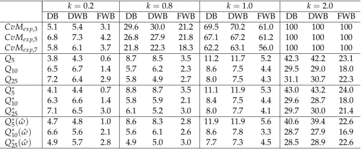
3.2 Empirical size ofQ∗mandQ∗∗m . . . 60
3.3 Empirical size ofQ∗m(ωˆ)andQ∗∗m(ωˆ) . . . 61
3.4 Density plots of portmanteau tests . . . 64
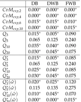
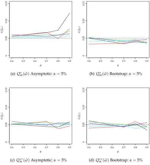
3.5 Estimated significance level forβ=5% whereφ= 0.9 . . . 68
5.1 Choices of the lasso tuning parameter . . . 102
5.2 Lasso solution path using the LARS algorithm . . . 104
5.3 Solution path of the lasso and adaptive lasso for regression . . . 119
5.4 Probability of true regression model on the solution path,εi ∼ Normal . 122 5.5 Probability of true regression model on solution path,εi ∼t . . . 124
5.6 Probability of true regression model on solution path,εi ∼χ2 . . . 125
5.7 Probability of true regression model on solution paths,εi ∼lognormal . 126 5.8 Median estimated regression model size . . . 128
5.9 Percentage of correct regression models . . . 130
5.10 Median of relative regression model error . . . 131
5.11 Boxplot of tuning parameter . . . 132
6.2 Median multivariate time series model size . . . 159 6.3 Percent correct models for multivariate time series . . . 160 6.4 Median of relative multivariate time series model error . . . 161
2.1 Mean and standard deviation of portmanteau tests. . . 38
2.2 Empirical size for AR(2)process . . . 40
2.3 Bootstrap empirical size for AR(4)process . . . 41
2.4 Power (in %) for AR(2)against ARMA(2, 2). . . 42
2.5 Empirical power against EXPAR(2). . . 44
2.6 Empirical power against TAR(2) . . . 45
2.7 p-values for Canadian lynx data . . . 46
3.1 Bootstrap empirical size for AR(1)process . . . 65
1 Bootstrap sampling procedure . . . 35
2 Computation of empirical size. . . 35
3 Computation of empirical power. . . 36
4 Coefficients of reciprocal of AR and MA polynomials . . . 52
5 Computation of weights of AR representation of an ARMA(p,q)process 54 6 Computation ofKatayama(2008) correction term for an ARMA(p,q)process 55 7 Nonlinear least squares estimation of ARMA(p,q)process . . . 55
Introduction
1.1
Introduction
A time series is a set of observationsyt, with each observation being recorded at
spec-ified timet(Brockwell and Davis,1991). Time series models have wide applications in science and technology. Examples of time series can be found in almost every field of life including, for example, economics, astronomy, physics, agriculture, genetic engi-neering and commerce.
Mathematical models play an important role in the statistical analysis of data. These models can be deterministic or stochastic. In time series analysis the first and most important step is to identify the appropriate class of mathematical models for the data. As in regression problems, model criticism is an important stage in time series model building, where the fitted model is under scrutiny. To improve the model, we need to go through an iterative procedure of identification, estimation and diagnostic checking. The diagnostic checking not only examines the model for possible shortcomings but it can also suggest ways to improve the model in the next iterative stage (Box and Jenkins, 1994, Chapter 8).
In this thesis, we are interested in goodness-of-fit tests used for diagnostic checking of linear time series models so we will only consider the linear time series with finite second order moment. We will mainly look at overall goodness-of-fit tests suggested in literature e.g. Box and Pierce(1970), Ljung(1986), Monti(1994), Escanciano(2007), Katayama (2008), Katayama (2009). The goodness-of-fit tests used to test the
signifi-cance of a group of firstm, say, autocorrelations are called portmanteau tests. A review of literature on goodness-of-fit tests is briefly given in Section 1.4 and discussed with more detail in Section2.2.1.
Variable selection, especially in high dimensional settings, is important to have the optimal subset of predictors. In regression we have methods, e.g. the lasso (Tibshirani, 1996), which can do variable selection and parameter estimation simultaneously. Vari-able selection sometimes lead to greater prediction accuracy (Hastie et al.,2001, p.57). These methods have not been widely discussed for time series models. In this thesis we have developed a novel approach to the use of lasso-type methods for multivari-ate time series analysis including a study of the oracle properties of our proposals. Thus we have mainly focused on two aspects of time series model building, namely (i) goodness of fit tests for diagnostic checking of time series models and (ii) applications of shrinkage methods to time series models.
The first part of this thesis includes numerical and theoretical results on time se-ries goodness-of-fit testing, which is an important part of model building. We study goodness-of-fit tests under their distribution based on first-order asymptotic theory (Ljung and Box,1978,McLeod,1978,Katayama,2008) and distribution approximated by a variety of bootstrap methods including dynamic (MacKinnon,2006) and fixed de-sign bootstrap methods (Escanciano,2007). We present some numerical results for the bootstrap distributions of these tests and also provide some theoretical justification of dynamic bootstrap methods. For details see Section2.3.1.
In the second part of the thesis, we investigate oracle properties (Fan and Li,2001) of lasso-type methods for regression and time series models. Firstly, we look at the implementation of the lasso (Tibshirani,1996) and adaptive lasso (Zou,2006) to linear regression models. We discuss the scenarios where the lasso does not achieve the oracle properties while the adaptive lasso does. We find the necessary and almost sufficient condition discussed byZou(2006) and Zhao and Yu(2006) is an important condition for consistent variable selection for these lasso-type methods. We also notice for the adaptive lasso that normalisation of the predictors after rescaling with the adaptive weights results in the adaptive lasso with uniform weights i.e. the standard lasso.
The properties of lasso-type methods are well studied for regression models, see e.g. Tibshirani (1997) discussed the application of lasso to Cox proportional hazard models, Van De Geer (2008) studied the application of the lasso to high-dimensional generalized linear models. But application of lasso-type methods to time series models is still in its early stages. Some discussion can be found on the ways to implement lasso-type methods to time series data, see e.g. Haufe et al. (2008), Gustafsson et al. (2005), Hsu et al. (2008), Nardi and Rinaldo (2008) but we cannot find any theoretical results in the time series setting.
Haufe et al. (2008) studied the sparse causal discovery of multivariate time series using simulation study. They compared the performance of group lasso (Yuan and Lin, 2006) and ridge regression (Hoerl and Kennard,1970) with multiple testing (Hothorn et al., 2008). Gustafsson et al. (2005) applied lasso to time series data of gene-to-gene net-work.Hsu et al.(2008) has shown good performance of the lasso for multivariate time series models in comparison to the conventional information-based AIC (Akaike,1974) and BIC (Schwarz,1978) methods. He also proved the asymptotic distribution of lasso estimates under vector autoregressive models. Nardi and Rinaldo (2008) has derived set of conditions when the lasso estimation is consistent in model selection, estimation and prediction but these results are proved for univariate autoregressive process.
We present the implementation of lasso-type methods to vector autoregressive mod-els. We prove the necessary condition for the consistent variable selection property of these methods. We also give theoretical proofs for the oracle properties of the adaptive lasso for time series models on the lines ofZou(2006). Our results show, as for regres-sion models, the oracle properties of the adaptive lasso also hold for stationary time series models.
The rest of this chapter is organised as follows: Section 1.2 gives some important definitions used in time series analysis. Important types of stochastic processes are defined in Section1.3. We will give a literature review of time series model diagnostic checking in Section1.4. Bootstrap methods are briefly defined in Section1.5. Finally, in Section1.6, we will define the importance of variable selection with a brief survey of popular methods used to do variable selection.
1.2
Some Definitions
Time series data have unique characteristics and importance as the dependence among the observations can be used to forecast the phenomenon for some future time. Time series analysis provides the tools for the analysis of this dependence. The use of time series stochastic and dynamic models play a vital role in this analysis. Assuming that, in time series each observation yt is a realization of a certain random variableYt, we
can consider the time series{yt}t≥1 as a realization of the family of random variables {Yt}t≥1. Now we define briefly some of the important types of time series models. Now we give some important definitions, for details see e.g. Box and Jenkins(1994).
Mean and Variance
IfYtis a stationary process, defined later in this section, with probability
distribu-tionp(yt)then the mean and variance are defined as
µ=E(Yt) = Z ∞ −∞ytp(yt)dyt, and σ2 =E(Yt−µ)2= Z ∞ −∞(yt−µ) 2 p(yt)dyt.
For the stationary time series{yt : t =1, . . . ,n}, the sample mean and variance can be
defined as ¯ y= 1 n n
∑
t=1 yt, and s2= 1 n n∑
t=1 (yt−y¯)2.Strict Stationarity
Let{yt}t≥1be an observed series of the stochastic process{Yt}t≥1then
FYt1,...,Ytn(y1, . . . ,yn) =P(Yt1 ≤y1, . . . ,Ytn ≤yn)
denote the joint distribution function ofYt1, . . . ,Ytn for anyt1,t2, . . .,tn ∈ Z. Then a
time series{Yt}is said to be stationary if for anyk∈Z, andn=1, 2, . . .
FYt1,Yt2,...,Ytn(y1, . . . ,yn) =FYt1+k,Yt2+k,...,Ytn+k(y1, . . . ,yn).
Thus, shifting the times of the observations backward or forward by an integer amount kdoes not affect the joint distribution. This definition is often termed strict stationarity, see e.g.Tong(1990).
Stationarity processes are considered to be in a state of equilibrium. Given the nor-mality assumption, stationarity is the primary assumption in time series analysis as a stationary process can be described by its mean, variance and spectral density function (Box and Jenkins,1994, p.43). In practical situations, stationarity may or may not hold, but there are various ways of transforming time series data to approximate stationarity, see e.g.Box and Jenkins(1994).
Weak Stationarity
A weaker form of stationarity is that the mean and variance of the process Yt are
constant and their autocovariance function, defined later in this section, does not de-pend on time t but only on lag k. This is also called second order stationarity as it requires conditions only up to the second order moment. Since a Gaussian process is fully characterised by its first and second order moments, for such processes weak sta-tionarity implies strict stasta-tionarity, see e.g.Box and Jenkins(1994).
Autocovariance and Autocorrelation Function
IfYtis a stationary process thenck does not depend ontand is defined as
ck =cov(Yt,Yt+k) =E(Yt−µ) (Yt+k−µ), k=0,±1,±2, . . . .
TheYtprocess is said to be white noise ifck = 0, when|k| ≥1. The autocorrelation at
lagkis
rk = ck
c0, k=0,±1,±2, . . . . (1.2.1)
For the stationary time series{yt : t = 1, . . . ,n}, the sample autocovariance function,
ˆ
ck at lagk, can be defined as
ˆ ck = 1 n n−k
∑
t=1 (yt−y¯) (yt+k−y¯), k=0,±1,±2, . . . .Note that divisor is used asninstead ofn−kto ensure that the matrix ˆC= [cˆi−j]ni,j=1is non-negative definite (Brockwell and Davis,1991, p.29) and thus for a stationary time series with finite second order moment, we can define autocorrelation function ˆrk, at
lagk, ˆ rk = ˆ ck ˆ c0 k=0,±1,±2, . . . . (1.2.2)
The estimated autocorrelation coefficients ˆrkare approximately independently and
iden-tically distributed (i.i.d.) with zero mean and
var(rˆk) =
1 n.
Note thatc0 = σ2andr0 = 1 and for the sample version ˆc0 = s2and ˆr0 = 1, whereσ2 is the variance of the process{Yt :t∈N}ands2is the sample variance.
Partial Autocorrelation Function
The partial autocorrelation function of a stationary process Yt with finite second
order moment,ωk, can be defined as the correlation betweenYtandYt+kafter removing
kth coefficient in the autoregressive representation of orderkof the jth autocorrelation coefficient
rj =φk1rj−1+. . .+φkkrj−k j= 1, . . . ,k. (1.2.3)
The sample partial autocorrelation can be defined in parallel to (1.2.3) as
ˆ
rj =φˆk1rˆj−1+. . .+φˆkkrˆj−k j= 1, . . . ,k,
thus ˆωk= φˆkk(Brockwell and Davis,1991, p.102).
Partial autocorrelation plays a vital role in determining the order of the autoregres-sive model underlying a time series, details given in definition of autoregresautoregres-sive mod-els in Section1.3. Under the hypothesis that the underlying process is autoregressive of order p, the estimated partial autocorrelation coefficients ˆωkof order greater than p
are approximately i.i.d. with zero mean and
var(ωˆk)≈ 1
n, k ≥ p+1, (1.2.4)
see e.g.Box and Jenkins(1994, p.68).
1.3
Some Important Types of Time Series
In this section we give definitions of some important time series models.
Moving Average model
A process
yt =β(L)εt, (1.3.1)
is called a moving average process of orderq, denoted as MA(q)process, where
and εt is a white noise sequence (see e.g. Box and Jenkins, 1994). The operator L is
called the lag operator such that LjYt = Yt−j. For finiteq, moving average processes
are always stationary and their autocorrelation functionrk, defined in (1.2.1), cuts off
to zero fork ≥ q+1. This is an important property of moving average processes and plays an important role in model identification underlying an observed sample time series.
Autoregressive model
A process
α(L)yt =εt (1.3.3)
is called an autoregressive process of orderp, denoted asAR(p)process, where
α(L) =1−α1L−α2L2−. . .−αpLp. (1.3.4)
An AR(p)process is said to be stationary when roots ofα(L) = 0 lie outside the unit circle or roots ofα(L−1) =0 lie inside the unit circle, where
α(L−1) =1−α1L−1−α2L−2−. . .−αpL−p.
The autocorrelation function of an AR(p)process is infinite in extent e.g. it can be a damped sine wave or an exponentially decaying curve. For example, for an AR(1)
process yt = φyt−1+εt, autocorrelation function shows an exponential decay if the
autoregressive parameter is positive i.e. 0<φ<1 while it makes a damped sine wave
if autoregressive parameter is negative i.e. −1 < φ < 0 (Box and Jenkins,1994, p.58)
But the partial autocorrelation function of AR(p) process is non-zero only for first p lags i.e.ωk =0 fork≥ p+1 (Brockwell and Davis,1991, p.100).
Autoregressive Moving Average model
A process
is called an autoregressive moving average process, denoted as ARMA(p,q)(see e.g. Box and Jenkins, 1994), where β(L)and α(L)are defined in (1.3.2) and (1.3.4) respec-tively. It is important to note that typically a stationary time series can be represented simultaneously by an autoregressive, moving average or mixed autoregressive moving average process of adequate order. The ARMA(p,q)model results in a more parsimo-nious model representation.
An ARMA(p,q)model can be represented in AR(∞)form as
π(L)yt= εt, (1.3.6)
where π(L) = α(L)β(L)−1 = ∑∞
i=0πiLi. We can also write ARMA(p,q) model in
MA(∞)form as
yt =ψ(L)εt, (1.3.7)
whereψ(L) =β(L)α(L)−1=∑∞
i=0ψiLi. See e.g.Wei(2006, Chapter 3),Brockwell and Davis
(2002, Chapter 6) for detailed discussion including the applications of linear models.
Autoregressive Integrated Moving Average model
Suppose we have a non stationary ARMA(p+d,q)process of the formα′(L)yt =
β(L)εt, such thatd roots ofα′(L) = 0 lie on the unit circle. In such situations we can
write it as a stationary processwtsuch thatα(L)wt= β(L)εt wherewt =∇dyt. We can
sayytis an ARIMA(p,d,q)andwtis an ARMA(p,q). Theα(L)andβ(L)are defined in
(1.3.4) and (1.3.2) respectively.
Non Linear Time Series Models
Many time series especially occurring in the natural sciences and engineering can-not be modeled by linear processes. These kinds of time series can have trends which can be best modeled by nonlinear processes. The model building process for nonlinear time series is much more complicated than for linear time series. The important types of nonlinear time series includes bilinear, threshold autoregressive, exponential autore-gressive, autoregressive conditional heteroscedastic (ARCH), generalized
autoregres-sive heteroscedastic (GARCH) and stochastic and random coefficient models see e.g. Fan and Yao(2003, Chapter 1),Li(2004, Chapter 5),Brockwell and Davis(1991, Chap-ter 13) andChatfield(2004, Chapter 11). Some of these models are defined in Section 2.4.
As we have discussed earlier, finite order moving average processes are always stationary, so in the analysis of these processes for uniqueness purposes we need some conditions on the parameters of the process. Here we give the definition of invertibility, an important condition on moving average processes.
Invertibility
A moving average process{Yt}is said to be invertible, if the roots ofβ(L) = 0 lie
outside the unit-circle whereβ(L)is defined in (1.3.2). The invertibility condition is in-dependent of the stationarity condition and can also be applied to non-stationary linear time series. Invertibility is required for uniqueness purposes as two normal stationary processes can have same autocorrelation function see e.g. Chatfield(2004, p.37).
1.4
Diagnostic Checking
As mentioned earlier, time series model building is a three stage iterative process con-sisting of identification, estimation and diagnostic checking. Once the model is identi-fied and fitted to an observed series, the next stage is to check the model for possible discrepancies.
One approach is to assume that the fitted model is under-fitted and so suggest a new model with some additional parameters. This method is called overfitting but the practical problem is to know the directions in which the model should be aug-mented. An analysis of the identified and overfitted model leads to the conclusion if the additional parameters are needed. Information criteria like Akaike information cri-terion (AIC) (Akaike, 1974) and Bayesian information criterion (BIC) (Schwarz, 1978) can be used for the final model selection. See McQuarrie and Tsai (1998, Chapter 3) Box and Jenkins(1994, Section 8.1.2) for details.
pos-sible discrepancies in the model and also to further suggest some modifications to the model. Residuals are analysed and checked if they satisfy the model assumptions. Any significant differences from the model assumptions mean we fail to prove that our fit-ted model is correct.
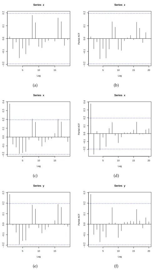
Residuals plots may be the first step to look at the patterns and behaviour of resid-uals. Residuals plots along with plots of residual autocorrelations and partial auto-correlations provide an important set of diagnostic tools. Any non random pattern on the residuals plot or any significant residual autocorrelation suggest modification in the fitted model. Figure 1.1shows that autocorrelations and partial autocorrelations for seriesz is lying within the confidence limits therefore we can consider seriesz as a purely random series. For seriesx, autocorrelation plot is cutting off after lag 1 and partial autocorrelation function is showing a damped sine wave pattern, a behaviour of moving average process of order 1. Similarly for seriesy, partial autocorrelation is dying off after lag 1 with autocorrelation showing a pattern of damped sine wave, so seriesycan be identified an autoregressive process of order 1. The identified moving average and autoregressive models should be considered as possible candidate models which can be further tested in the iterative procedure of model building.
The autocorrelation (partial autocorrelation) plot of the residuals is the graph where residuals autocorrelations up to some finite lag, say m, are plotted along with large sample confidence limits. Any autocorrelation (partial autocorrelation) lying outside these limits indicates some non randomness in the residuals. Instead of testing the significance of individual autocorrelations,Box and Pierce(1970) suggested a portman-teau test for the firstmautocorrelations. Later, several modifications of Box-Pierce were suggested in the literature. A survey of these tests is given in Section2.2.1.
In the following section, we give a brief review of some bootstrap methods which are commonly used for time series models, but before that we give a description of the Monte Carlo method.
Since the paper byMeteopolis and Ulam(1949) and the advent of high speed com-puters, the Monte Carlo method has been applied in almost every field of science e.g. physics, biological sciences, finance etc. Monte Carlo methods use repeated sampling
5 10 15 −0.1 0.0 Lag A CF Series z − 0. 2 0. 1 0. 2 (a) 5 10 15 20 −0.1 0.0 Lag P ar tial A CF Series z − 0. 2 0. 1 0. 2 (b) 5 10 15 −0.1 0.0 Lag A CF Series x − 0. 2 0. 1 0. 2 0. 3 0. 4 (c) 5 10 15 20 −0.1 0.0 Lag P ar tial A CF Series x − 0. 2 0. 1 0. 2 0. 3 0. 4 (d) 5 10 15 −0.1 0.0 Lag A CF Series y − 0. 2 0. 1 0. 2 0. 3 (e) 5 10 15 20 −0.1 0.0 Lag P ar tial A CF Series y − 0. 2 0. 1 0. 2 0. 3 (f)
Figure 1.1: Examples of autocorrelation function and partial autocorrelation functions.
and provide an efficient numerical method to solve a statistical problem for example, we can obtain the first few moments of a distribution even without having any priori knowledge of this distribution. For details seeRobert and Casella(2004).
1.5
Bootstrap Methods
In practice, we come to situations when it is very hard or sometimes impossible to work out the asymptotic distribution of an estimator. In these situations, an approximation of the asymptotic distribution can be obtained by a resampling method. Though the concept of bootstrap methods goes back to the 1930s,Efron(1979) first introduced it in a unified way.
Bootstrap methods are based on a simple idea that the relation between population and sample can be recreated by resampling from the sample. Bootstrap methods pro-vide mechanisms to generate bootstrap samples. The concept of bootstrap methods is quite simple in the case of i.i.d. random variables but the situation becomes compli-cated for time series data (Lahiri,2003).
One way to resample from time series data is the block bootstrap method where the
sample is divided into blocks, overlapping (K ¨unsch,1989) or non-overlapping (Politis and Romano, 1992), of a certain length. Block length is an important issue and is chosen such that
the dependence structure in the original sample can still be explained by the bootstrap sample. Under the stationarity condition each block should have the same joint prob-ability distribution. Block bootstrapping is a non parametric bootstrap method. There are some other parametric and semi parametric bootstrap methods for time series data. Assuming that we have some knowledge of the underlying distribution, say Gaussian, the parametric bootstrap is sampling from the estimated distribution.
Semi parametric bootstrap methods use the model structure to resample the resid-uals. The residuals are obtained by fitting the model to time series data. The residuals can be considered approximately i.i.d.. Having the resamples of these residuals, we can use the fitted model to obtain the bootstrap samples of the time series. Sometimes, residuals may require some transformation for centering and scale adjustment, see e.g. Stute et al.(1998).
1.6
Variable Selection
In the second part of our thesis we look at the implementation of shrinkage methods to regression and time series. Here we briefly introduce these methods, mainly in the context of regression analysis. Later in Chapter 5, we will implement some of these methods in the regression setting while application to time series data will be discussed in Chapter6.
Discovering the relationships between the response variable{yi :i=1, . . . ,n}and
the set of predictors {xj : j = 1, . . . ,p} is one of the objectives of regression analy-sis. This relationship is later used for statistical inference and prediction. The linear regression model is usually defined as:
yi = β0+β1xi1+. . .+βpxip+εi, i=1, . . . ,n.
In vector form, we can write the model as
yi =β0+xiTβ+εi (1.6.1)
such thatyi ∈Ris the response variable,xi = (xi1, . . . ,xip)T ∈Rpis thep-dimensional
set of predictors,εi ∼N(0,σ2)andβ= (β1, . . . ,βp)is the set of parameters andβ0is a constant.
The ultimate question is to estimate the βj’s using a set of training data (xT1,y1), . . ., (xTn,yn), where xi = (xi1, . . . ,xip)T ∈ Rp. The method of least squares, based
on minimising the residual sum of squares, is the most popular method to estimate the model. The least squares estimates always provide non-zero estimates even if true model is sparse i.e. some of the model parameters are exactly zero. This is the reason that least squares estimates generally have low bias but may suffer from large predic-tion variance especially when true model is sparse. The large predicpredic-tion variance is due to the fact that least squares estimation always ends up with the full model see e.g. Hastie et al.(2001, p.57).
1.6.1 Subset Selection
In model building, we often have a large set of predictors. As all the variables are not equally important for the model, so we seek for a parsimonious model. The parsimo-nious models are very important for prediction purposes as overfitted models some-times have the higher prediction variance see e.g. McQuarrie and Tsai (1998, Section 1.2),Hastie et al.(2001, p.57).
Variable selection in regression is so important that Bradley Efron, the inventor of bootstrap methods, has named it as one of the most important problems in statistics (Hesterberg et al.,2008). All the predictors, in general, are not worth to include in the model especially whenpis very large. We look for a subset of{βj : j=1, . . . ,p}which
optimizes a criterion, see Hocking and Leslie (1967). This criterion can be based on certain model goodness measures like prediction error, goodness of fit measures or on estimating some measures of distance between the model based on the subset and the true model, see e.g. Seber and Lee(2003).
Searching through all possible subset models is computationally intensive. Best subset selection produces a model that is interpretable and has possibly lower predic-tion error than the full model. It is one way to fit a simple model but, as menpredic-tioned by (Fan and Peng,2004), is not feasible with a large set of predictors. Methods such as for-ward stepwise selection and backfor-ward elimination, called greedy algorithm, provide a good path through them (Hastie et al.,2001, p.58). More recently, there are sugges-tions e.g.Hall et al.(2009b) andCho and Fryzlewicz(2010) based on tilting for variable selection in high-dimensional setting.
Shrinkage methods are another choice which lead to a simpler model in terms of number of variables in the model. In the following section, we give a review of some of the important shrinkage methods.
1.6.2 Shrinkage Methods
Subset selection is a discrete process i.e. either a candidate variable is included or ex-cluded from the model. Thus a model, though simpler, can have a relatively high pre-diction variance. Shrinkage methods answer this problem in an opposite way i.e. retain
all the predictors but use a penalised least squares method instead of standard least squares estimation. The concept of shrinkage was first introduced by James and Stein (1961). Shrinkage is desired when a simpler model is desired at a cost of increased pre-diction error but this increase is relatively lesser than result for a discrete process like subset selection. Here we give some brief description of some of the shrinkage meth-ods. For more detailed discussion see Section5.2.
Ridge Regression
Ridge regression (Hoerl and Kennard,1970) is a form of shrinkage method, which shrinks the coefficients by imposing a penalty on the sum of squares of the parameters. Ridge regression was primarily suggested for improving the estimation of regression coefficients when the predictors are highly correlated. We can also define ridge regres-sion as a mean or mode of a posterior distribution of response variable with a suitable chosen of prior distribution for regression parameter, in which case we can see that op-timal performance of ridge regression much depends on the distribution of regression coefficients , see e.g.Hastie et al.(2001, p.64). One drawback of ridge regression is that it fails to produce a simple model as it retains all the variables, see e.g. Seber and Lee (2003). Ridge regression is preferred to variable subset selection when objective is to minimize prediction error (Frank and Friedman,1993).
Garrote
Shrinkage and simple models are desired simultaneous for an interpretable model with low prediction variance (Hastie et al.,2001, Section 3.4). Subset selection provides the simpler model but fails to shrink while ridge regression shrinks the regression coef-ficients but retains all the variables in the model. Garrote (Breiman,1995) does shrink-age while setting some the coefficients exactly to zero at the same time. Garrote puts a penalty on each individual least squares estimate ofβj’s. As the penalty term increases
the shrinkage coefficients get smaller and some are even forced to zero. Due to the condition on the shrinkage coefficient to be nonnegative this version of garrote is also called nonnegative garrote, this condition was further relaxed byBreiman(1996).
Lasso
The lasso (Tibshirani,1996), least absolute shrinkage and selection operators, is an L1 penalised least squares regression. Like garrote it shrinks some of the coefficients while setting the rest of them exactly to zero. This property of the lasso makes it a method which enjoys good properties of best subset regression and ridge regression (Hastie et al.,2001, p.82) The lasso estimator ofβfor model (1.6.1) is defined by
ˆ β∗j =argmin n
∑
i=1 yi−β0− p∑
j=1 βjxij !2 +λ p∑
j=1 |βj| , j=1, . . . ,p,whereλ> 0 is a user-defined tuning parameter. The choiceλ = 0 corresponds to the
least squares estimate and larger values of λresult in a higher amount of shrinkage i.e. relatively more variables will shrink to zero. The theoretical properties of the lasso method are very appealing but it had been computationally expensive untilEfron et al. (2004) suggested an efficient least angle regression (LARS) algorithm for finding the solution path of the lasso method. The LARS correctly organizes the calculations thus the computational cost of the entirepsteps is of the same order as that required for the usual least squares solution for the full model.
Variable selection is an important property of shrinkage methods. Zou(2006) and Zhao and Yu(2006) has discussed a necessary condition for the lasso methods to achieve consistency in variable selection. Zou (2006) has also suggested the use of adaptive weights and showed that this results in putting a different penalty on each parameter, which leads to consistent variable selection. The same LARS algorithm (Efron et al., 2004) can be used to obtain the adaptive lasso estimates, see Section5.2.4for detailed discussion on the adaptive lasso.
The rest of this thesis is organised as follows:
Goodness of fit testing is an important stage of time series model building. In Chap-ter2, we study the properties of time series goodness of fit tests. Though these prop-erties are well studied but there is not much literature available studying these tests especially for semi-parametric bootstrap methods. We give some numerical results to compare the performance of various resampling residuals approaches in providing an
approximation of finite sample distributions underlying these tests. We also compared the power of these tests against various linear and non-linear alternative models.
Katayama (2008) derived a bias term in Ljung-Box test. This motivated us to com-pare Katayama’s bias corrected Ljung-Box test with other goodness-of-fit tests using asymptotic and dynamic bootstrap method. In Chapter 3, we numerically study the effect of the Katayama (2008) bias correction term in the Ljung and Box (1978) port-manteau test. We also suggest a set of algorithms to estimate this bias correction term. In this same Chapter 3, we present a novel suggestion for a bias correction term in Monti(1994) test on the lines ofKatayama (2008). Chapter 3also includes numerical results on Katayama’s suggested multiple test (Katayama,2009). We suggest a hybrid bootstrap approach to estimate the joint significance levels of this multiple portman-teau test. We also suggest the use of pivotal portmanportman-teau test and an algorithm for its efficient computation.
The results in Chapter 2 lead to the conclusion that dynamic bootstrap sampling provide an approximation of the finite sample distribution better than first order asymp-totic theory. This motivated us to provide a theoretical justification of this finding. In Chapter 4, where we have provided theoretical insight of good performance of dy-namic bootstrap methods in estimating the distribution of the portmanteau tests espe-cially whenmis small and the process is close to stationarity boundary. We provide a set of lemmas to prove the asymptotic normality of the least squares estimates. We have proved the bounds on the cumulants of the residuals which are used to derive the nor-mality of bootstrap least squares estimates. We discuss an approach to use these results as a justification of good performance of dynamic bootstrap method for portmanteau tests. We, along the lines ofKatayama(2008), derive and suggest a bias correction term in Monti’s(1994) test.
Issues like selection of tuning parameter for these shrinkage methods and condi-tions required to achieve oracle performance by these methods are still areas of interest. In the second part of our thesis, we look at the oracle properties of lasso-type methods. In particular, we study the property of consistent variable selection for these methods. In Chapter5, numerical results on variable selection of the lasso (Tibshirani,1996) and adaptive lasso (Zou,2006) are given and discussed. We present some interesting
nu-merical results about the selection of the tuning parameter. Lasso-type methods are originally suggested for linear regression models and their theoretical properties are proved in the regression context (see e.g.Knight and Fu,2000).
Shrinkage methods are now widely used in regression setting but it is less explored for time series setting. Though time series models have some similarities with regres-sion models, the results are not trivial (see e.g. Anderson, 1971). In Chapter 6, we apply lasso-type methods to the multivariate time series models. We also give some novel results about the application of these methods to linear time series models. Like regression, we derive a necessary (but not sufficient) condition for consistent variable selection by lasso-type methods. We prove the asymptotic normality of the adaptive lasso and show that the adaptive lasso is always consistent in variable selection.
Finally, in Chapter 7, we give a summary and conclusion of our results. Future directions of our work are also discussed in this same chapter.
Bootstrap Goodness of Fit Tests for
Time Series Models
2.1
Introduction
In this chapter, we mainly look at the properties of goodness-of-fit tests for linear time series models under semi-parametric bootstrap methods. Model criticism is an im-portant stage of model building and thus goodness of fit tests provide a set of tools for diagnostic checking of the fitted model. Box and Pierce (1970) test and its sev-eral other versions are perhaps the most commonly used type of portmanteau test (Mainassara et al.,2009). The portmanteau tests are used as overall tests for an entire set of, say, the firstmautocorrelations assuming that the true model is correct.
The asymptotic distribution of these tests is well studied in the literature and many researchers have questioned the appropriateness of theχ2
m−p−qdistribution as its
ap-proximation under ARMA(p,q)as a true model, see e.g. Katayama(2008) and refer-ences therein. Moreover, the choice ofmis very important in theχ2m−p−qapproximation and power of these tests.
In this chapter, we numerically study the size and power of some of the popu-lar time series goodness of fit tests. Escanciano(2006b) has studied power of various goodness of fit tests under the fixed design wild bootstrap. Horowitz et al.(2006) has compared performance ofBox and Pierce(1970) test with some other tests under block-of-block bootstrapping. See Section2.3.1for more detailed discussion.
Most of the literature in time series bootstrap goodness-of-fit tests is related to non-parametric bootstrap methods. Results inEscanciano(2007) andKatayama(2008) moti-vated us to look at size and power properties of these goodness-of-fit tests for bootstrap methods using resampling residuals. The novelty of our study is that we study the size of the tests under various semi-parametric bootstrap designs described in Section2.3.1. Moreover, we also compare the power of these tests with the Cramer von Mises (CvM) (Escanciano, 2007) statistic against various linear and non-linear alternative models. We also study size and power of various versions of Box-Pierce test, Monti(1994) test and CvM test. To the best of our knowledge, these tests have not been compared in these scenarios in the literature.
Our results show that Box-Pierce type tests do well against the linear alternatives but fail to perform against the non-linear alternatives, while the situation reverses for the CvM statistic due toEscanciano(2007), i.e, the CvM statistic does well against non linear alternatives but much less well against linear alternatives. Moreover, dynamic bootstrap methods show better performance than the fixed design bootstrap in our example. We have not found any advantage of using wild residuals in our simulations. The remainder of the chapter is organized as follows. In the next section a review of the literature on available diagnostic tests is given. Section2.3describes the different bootstrap methods in a time series context. Section2.4gives the estimation procedure and algorithms for Monte Carlo simulations for computing the size and power of the tests. Finally, Section2.5 presents the results of simulations and discussion of the re-sults.
2.2
Literature Review
In practice, there are many possible linear and non-linear models for a problem under study e.g. autoregressive, moving average, mixed ARMA models, threshold autore-gressive etc. Box and Jenkins (1994) have described time series model building as a three-stage iterative procedure that consists of identification, estimation and valida-tion.
of identifying the underlying model though there are some tools, for example, the auto-correlation and partial autoauto-correlation plots to identify the general class of underlying model, seeBox and Jenkins(1994, p.196). See Section1.3for the definitions of autocor-relation and partial autocorautocor-relation. Importantly, it should be noted that at the identifi-cation stage, especially dealing with complex situations, we identify a class of models that will later be efficiently fitted and then go through the diagnostic checking phase (Box and Jenkins,1994). Identification of a single model makes the practitioner assume that the data are generated under this particular identified model. To overcome this problem, model averaging methods such as Bayesian model averaging can be used see e.g.Hoeting et al.(1999) and references therein.
There are rigorous ways to estimate the parameters of autoregressive models such as the methods of maximum likelihood estimation, least squares estimation and Yule-Walker estimation. Moving average models can be estimated through the innovations method, see e.g.Brockwell and Davis(1991, Chapter 8). The estimates of moving aver-age models and the mixed models can also be obtained graphically or through iterative estimation procedures such as non-linear minimization (see e.g.Box and Jenkins,1994, Chapter 7).
Time series models should be able to describe the dependence among the observa-tions, see e.g. Li(2004). It is a well-discussed issue that in time series model criticism, the residuals obtained from fitting a potential model to the observed time series play a vital role and can be used to detect departures from the underlying assumptions, (Box and Jenkins,1994;Li,2004).
In particular, if the model is a good fit to the observed series then the residuals should behave somewhat like a white noise process. So, taking into account of the ef-fect of estimation, the residuals obtained from a good fit should be approximately un-correlated. While looking at the significance of residual autocorrelations, one approach is to test the significance of each individual residual autocorrelation which seems to be quite cumbersome. Another approach is to have some portmanteau test capable of testing the significance of the first, saym, residual autocorrelations (Box and Jenkins, 1994;Li,2004), an approach we now describe.
2.2.1 Diagnostic Tests
Since Box and Pierce(1970) paper, the portmanteau test has become the vital part of time series diagnostic checking. Several modifications and versions of Box and Pierce (1970) has been suggested in the literature, see e.g. Ljung and Box(1978),McLeod and Li (1983), Monti (1994), Katayama (2008), Katayama (2009). These tests are capable of testing the significance of the autocorrelations (partial autocorrelations) up to a finite number of lags.
The third stage of diagnostic checking process (Box and Jenkins,1994) provides a practitioner an opportunity to test the model before using it for forecasting. This stage not only checks the fitted model for inadequacies but can also suggest improvements in the fitted model in the next iteration of this model building procedure. In this section we will do a literature review of the available diagnostic tests for fitted time series models.
The residuals are very commonly used as a diagnostic tool to test the goodness of fit of models. In a time series context, if the fitted model is good then it should be able to explain the dependence pattern among successive observations. In other words, all the dependence in terms of autocorrelations and partial autocorrelations of the data generating process (DGP) should be explained by the fitted model so there should be no significant autocorrelation and partial autocorrelation in successive terms of the residuals.
In practice the most popular way for diagnostic checking a time series model is the portmanteau test, which tests whether any of a group of the first m autocorrela-tions(r1ˆ , . . . , ˆrm)of a time series are significantly different from zero. This type of test
was first suggested by Box and Pierce (1970), in which they studied the distribution of residual autocorrelations in ARIMA processes defined in Section 1.3. Based on the autocorrelations of the residuals obtained by fitting an ARMA(p,q)model defined in Section1.3.5to{yt}, they suggested the following portmanteau test
Qm =n m
∑
k=1 ˆ r2k, (2.2.1)op-timal choice of m is difficult as the use of theχ2m−p−q approximation and diagnostic checking require large values ofmwhich results in less power and unstable size of test, as noticed by Ljung(1986), Katayama (2008). Katayama (2009) suggested a multiple portmanteau test to overcome this problem, for details see Section3.4.
Box and Pierce(1970) suggested thatQm ∼ χ2m−p−q, for moderate values ofmand
the fitted model is adequate, under the following conditions: 1. ψj ≤O n−1/2
forj≥m−p, and
2. mn =O n−1/2,
whereψj are the weights in the MA(∞)representation as defined in (1.3.7). This
ap-proximation requires substitution of residuals, ˆεt, for the error term, εt, in the model
but erroneous use of such kind of substitution can lead to a serious underestimation of significance level in diagnostic checking, see (Pierce,1972) and references therin. Many other researchers have also questioned the distribution ofQm, (see e.g. McLeod,1978
and references therein). The choice ofmis an important issue.
In the discussion of Prothero and Wallis(1976), Chatfield has mentioned the poor power properties ofQmand has recommended focusing on residual autocorrelations at
the first few lags and seasonal lags. Similar suggestions are also made by Davies et al. (1977). In the same discussion on the Prothero and Wallis paper, Chatfield and New-bold also pointed out the poor approximation of the finite-sample distribution ofQm.
Prothero and Wallis (1976), in their reply to this discussion, suggested the use of the correction factor (n+2)/(n−k)to Qm. However, this correction factor may inflate
the variance of the resulting statistic relative to that of the asymptoticχ2m−p−q
distribu-tion (see e.g.Davies et al.,1977,Ansley and Newbold,1979).
An important point to note is that the statisticQmhas been developed assuming the
normality of the white noise processεt. As the results ofAnderson and Walker(1964)
suggest the asymptotic normality of the autocorrelation of a stochastic process is inde-pendent of the normality of the stochastic process and only depends on the assumption of finite variance, so the portmanteau test is expected to be insensitive to the normality assumption.
Ljung and Box(1978) suggested the use of the modified statistic Q∗m =n(n+2) p
∑
k=1 ˆ r2 k n−k. (2.2.2)They have shown that the modified portmanteau statisticQ∗mhas a finite sample
distri-bution which is much closer toχ2m−p−q. Their results also show thatQ∗mis insensitive to
the normality assumption ofεt. As pointed out by many researchers e.g. Davies et al.
(1977),Ansley and Newbold(1979), the true significance levels ofQmtends to be much
lower than predicted by the asymptotic theory and though the mean of Q∗m is much closer to the asymptotic distribution, this corrected version of the portmanteau test has an inflated variance. But Ljung and Box(1978) pointed out that approximate expres-sion of variance given byDavies et al.(1977) overestimates the variance ofQ∗m.
Frequently in the literature larger values ofmhave been used inQmandQ∗m, and the
most commonly suggested value ism=20 (see e.g.Davies et al.,1977,Ljung and Box, 1978).Ljung(1986) suggests the use of smaller values ofmand has shown that for small values ofm,Q∗mhas an approximateaχ2bdistribution, whereaandbare constants to be
determined.
Ljung and Box (1978) also studied the empirical significance levels and empirical powers ofQ∗mfor various choices ofmand showed that the empirical significance lev-els for an AR(1)process are close to the nominal level for small choices ofm(m = 10 or 20) in all the cases except when the AR parameter is close to the boundary of non-stationarity region. This is a very challenging scenario for theχ2 approximation. We will look at this issue in Chapter3.Ljung and Box(1978) also showed that approximat-ing asymptotic distribution ofQm ∼ χ2ν, where ν = E(Qm)results in performance of
Qm similar to that ofQ∗m ∼χ2m−p−q.
We have already mentioned that the partial autocorrelation function is an important tool in determining the order of an autoregressive process (Quenouille,1947). The port-manteau testsQmandQ∗mare based on the autocorrelations. Monti(1994) suggested a
portmanteau test Q∗m(ωˆ) =n(n+2) m
∑
k=1 ˆ ωk2 n−k, (2.2.3)where ˆωkis the residual partial autocorrelation at lagk. She showed thatQ∗m(ωˆ),
anal-ogously to Q∗m, has an asymptotic null distribution χ2m−p−q and that Q∗m(ωˆ) is more
powerful thanQ∗mespecially when the order of the moving average component is
un-derstated.
As we have discussed earlier, the asymptotic distribution of Qm andQ∗m is
ques-tioned by several authors in the literature. Though small values ofmsolve this problem in some situations, it does not work in all cases, for example when the process is nearly stationary, seeLjung(1986). In a very recent paper,Katayama (2008) has suggested a bias correction term, in theLjung and Box(1978) statisticQ∗m, defined as
B∗m,n=rˆTV DVrˆ,
where ˆr = (r1ˆ , . . . , ˆrm)T, V = diag
p
n(n+2)/(n−1), . . . ,pn(n+2)/(n−m), D = X XTX−1XT and X is an (m×(p+q)) matrix partitioned into p and q columns, such that each(i,j)element of the partitioned matrix ofX is given
X = (−α∗i−j...−β∗i−j)
whereα∗i andβ∗i are defined by 1 α(L) = ∞
∑
i=0 α∗iLi and 1 β(L) = ∞∑
i=0 β∗iLiandα∗i = β∗i = 0 fori <0. Katayama(2008) showed the importance of this correction
term especially for small values ofmand when the roots of the ARMA(p,q)process lie near the boundary of non-stationarity region. So the bias corrected portmanteau test is given by
For more discussion onKatayama(2008), see Chapter3.
McLeod(1978, Theorem 1) has showed that ˆris approximately normal with mean 0andVar(rˆ) = (I−C)/n, whereC = XJ−1X,I is the identity matrix andJis the Fisher information matrix defined in (3.3.1). We noticed that approximation ofC by D = X(XTX)−1X, especially whenmis small, is a source of bias in approximating the asymptotic distribution of portmanteau tests. We found the use of pivotal statistic automatically corrects for the bias mentioned inKatayama(2008). Pivotal statistics are useful as their asymptotic distribution does not depend on unknown parameters, for details see e.g.Hall(1992, Ch.3). For more details see Section3.3.
Katayama (2008) suggested a multiple portmanteau test is based on several port-manteau test for a range of small to medium values ofm. He also discussed the linkage between his suggested multiple test and the test due to Pena and Rodriguez (2002). He suggested a method based on some iterative procedure to approximate joint distri-bution of the multiple test as the computation of the distridistri-bution is very hard due to correlated elements. See Section3.4for details.
For the past few decades the interest of researchers, especially working in the field of financial time series, has been focused on nonlinear models. It has been pointed out by several researchers that the Box-Pierce type tests fail to show good power against nonlinear models (see e.g.Escanciano,2006b;Pena and Rodriguez,2002). One impor-tant difference between nonlinear and linear models is that former do not inherit prop-erties of innovations e.g. a GARCH model with Gaussian innovations does not have to have a finite order fourth moment, for more detailed discussion see e.g. Fan and Yao (2003, Chapter 4).McLeod and Li(1983) used the sample autocorrelation of the squared residuals to test for linearity against the nonlinearity and showed its good power against departures from linearity.
Escanciano(2007) proposed diagnostic tests based on the CvM test using the weights suggested byBierens(1982), given by
CvMex p,P= 1 nσˆ2 n
∑
t=1 n∑
s=1 ˆ εtεˆsexp −12|It−1,P−Is−1,P|2 , (2.2.4)where ˆσ2=∑nt=1εˆ2t/n−1 is the variance of residuals and
It−1,P = (yt−1,yt−2, . . . ,yt−P) (2.2.5)
is the information set at timet−1 and dimensionP. It can be noticed that the distance |It−1,P−Is−1,P|2increases very fast withPwhich results in weights being near 0 when
Pis relatively large. We have considered theCvMstatistic with this weight scheme in our study as it has shown good power properties reported inEscanciano(2006b).
2.3
Methodology
We now consider various versions of the statistics defined in (2.2.1), (2.2.2), (2.2.3) and (2.2.4). We compare empirical size and power of these tests against various linear and non-linear classes of models. Mainly we compare the dynamic and fixed design boot-strap methods but we also look at the usefulness of transformed residuals in bootboot-strap methods.
2.3.1 Bootstrap Methods
Bootstrap methods are used to estimate the distribution of a test statistic or an esti-mator. The bootstrap is usually implemented using resampling. Under conditions that hold in wide variety of applications, the bootstrap provides approximations to distribu-tions of statistics that are at least as accurate as, and sometimes are more accurate than, the approximations of first-order asymptotic distribution theory (seeHardle et al.,2003). The reliability of a bootstrap method depends upon the extent to which the bootstrap data generating process (DGP) mimics the true DGP (seeMacKinnon,2006).
The bootstrap method was first suggested byEfron(1979) as a more general method than jackknife. For a detailed discussion on jackknife methods see e.g. Shao and Tu (1995). The idea of bootstrapping residuals was described inEfron(1988) in the context of regression. Much of the earlier work in bootstrap methods was done on i.i.d. random variables data.
ap-ply the bootstrap methods. In general, there are two main bootstrap methods that are used in time series i.e. model-based bootstrap methods and block-resampling boot-strap methods. Generally, the model-based bootboot-strap methods are called resampling-residuals bootstrap methods.
In block bootstrapping, we divide the sample into overlapping or non-overlapping blocks of a certain length (Hall et al.,1995). The performance of block bootstrap meth-ods much depend on block length. Under the stationarity condition each block should have the same joint probability distribution. In our study we consider only the model-based bootstrapping, as model-model-based bootstrap methods tend to be more accurate than block bootstrap methods (Lahiri, 2003) and also as our objective is to compare two model-based bootstrap methods, namely dynamic bootstrap and fixed design boot-strap.Lahiri(1999) provides a good comparison of block bootstrap methods with non-random and non-random block lengths.
Suppose we have a sample time series{yt}nt=1generated by a DGP defined by
yt = f(It−1,P,θ) +ǫt, (2.3.1)
whereIt−1,Pis the information set defined earlier in (2.2.5) andθis the vector of model parameters. Suppose the fitted model is
ˆ
yt= f It−1,P, ˆθ
, t= P,P+1, . . .
where ˆθis the estimate ofθ. Thus the residuals are
ˆ
εt= yt−yˆt, (2.3.2)
We assume that initial datayt−P, . . . ,y0are available.
Fully parametric bootstrap method
If the distribution of the error term, εt, is assumed to be known up to unknown
parameters, then we can use the knowledge of the distribution to select a bootstrap sample. Suppose, for example, thatεt ∼ N(0,σ2)then the bootstrap DGP will be given
as, y†t = fIt−† 1,P, ˆθ +ε†t, t =1, 2, . . . where ε† t ∼ N(0,σ2), σ2 is known and It†−1,P = y†t−1, . . . ,y†t−P is the parametric bootstrap ofIt−1,Pdefined in (2.2.5). If the true parameters are unknown then respec-tive maximum likelihood estimates are used for these unknown parameters (Chernick, 1999, p.124)
Semi-parametric time series bootstrap methods
Under the assumption that the DGP given in (2.3.1) is the true model for the given sample time series, the residuals given in (2.3.2) will serve the purpose of an i.i.d. sam-ple. The following approaches are used in semi-parametric time series bootstrap meth-ods.
Dynamic bootstrap If the error terms, εt’s, in our DGP are i.i.d., with common
vari-anceσ2, then we can generally make very accurate inferences by using the the dynamic bootstrap (DB) (MacKinnon,2006). This method requires the i.i.d. assumption of the error term and only mild conditions on its distribution. The DB is defined as:
y∗t = f It∗−1,P, ˆθ
+ε∗t fort =1, 2, . . . ,n, (2.3.3)
whereIt−∗ 1,P = y∗t−1, . . . ,y∗t−Pis the dynamic bootstrap of the information set defined in (2.2.5) andε∗t is selected at random with replacement from the vector of the residuals
(εˆ1, ˆε2, . . . , ˆ