University of Tennessee, Knoxville
Trace: Tennessee Research and Creative
Exchange
Masters Theses Graduate School
8-2013
A Multi-echelon Inventory System with Supplier
Selection and Order Allocation under Stochastic
Demand
Cong Guo
[email protected]This Thesis is brought to you for free and open access by the Graduate School at Trace: Tennessee Research and Creative Exchange. It has been accepted for inclusion in Masters Theses by an authorized administrator of Trace: Tennessee Research and Creative Exchange. For more information, Recommended Citation
Guo, Cong, "A Multi-echelon Inventory System with Supplier Selection and Order Allocation under Stochastic Demand. " Master's Thesis, University of Tennessee, 2013.
To the Graduate Council:
I am submitting herewith a thesis written by Cong Guo entitled "A Multi-echelon Inventory System with Supplier Selection and Order Allocation under Stochastic Demand." I have examined the final electronic copy of this thesis for form and content and recommend that it be accepted in partial fulfillment of the requirements for the degree of Master of Science, with a major in Industrial Engineering.
Xueping Li, Major Professor We have read this thesis and recommend its acceptance:
James Ostrowski, Mingzhou Jin
Accepted for the Council: Carolyn R. Hodges Vice Provost and Dean of the Graduate School (Original signatures are on file with official student records.)
A Multi-echelon Inventory System
with Supplier Selection and Order
Allocation under Stochastic Demand
A Thesis Presented for the
Master of Science
Degree
The University of Tennessee, Knoxville
Cong Guo
August 2013
c
by Cong Guo, 2013
Acknowledgements
I would like to express my sincere gratitude to my advisor, Dr. Xueping Li, for his guidance into my research life. I sincerely thank him for giving me the opportunity to be part of his research group and for his persistent support and understanding. I would also like to thank my thesis committee members: Dr. Mingzhou Jin and Dr. James Ostrowski, for helping me complete this thesis through all my hurdles.
I am grateful to all my colleagues in the Department of Industrial Systems Engineering who have assisted me in the course, and shared their graduate school life with me.
Last, but certainly not the least, I would like to acknowledge the commitment, sacrifice and support of my parents, who have always motivated me.
Abstract
This article addresses the development of an integrated supplier selection and inventory control problems in supply chain management by developing a mathematical model for a
multi-echelon system. In particular, a buyer firm that consists of one warehouse and N
identical retailers wants to procure a product from a group of potential suppliers, which may require different price, ordering cost, lead time and have restriction on minimum and maximum total order size, to satisfy the stochastic demand. A continuous review system
that implements the order quantity, reorder point (Q, R) inventory policy is considered
in the model. The objective of the model is to select suppliers and to determine the
optimal inventory policy that coordinates stock level between each echelon of the system while properly allocating orders among selected suppliers to maximize the expected profit. The model has been solved by decomposing the mixed integer nonlinear programming model into two sub-models. Numerical experiments are conducted to evaluate the model and some managerial insights are obtained by performing some sensitivity analysis.
Table of Contents
1 Introduction 1
2 Literature Review 5
3 Problem Definition and Assumptions 10
4 Model Formulation 16
4.1 Mathematical Model . . . 16
4.2 The Retailer Inventory Analysis . . . 19
4.3 The Warehouse Inventory Analysis . . . 21
4.4 Solution Procedure . . . 23
5 Illustrative Example and Analysis 27 5.1 Parameter Setting. . . 27
5.2 Results Analysis. . . 29
5.3 Demand Rate Analysis . . . 31
6 Conclusions 41
Bibliography 43
List of Tables
5.1 Parameter values assigned in the experiment . . . 28
5.2 Other parameter settings related to potential suppliers . . . 29
5.3 Decision-making variables solution. . . 30
5.4 The optimal policy and expected profit based on different demand rate instance 31
5.5 The optimal inventory policy for selected suppliers in different demand rate instances . . . 33
List of Figures
3.1 Illustration of the multi-level supplier selection system . . . 11
5.1 Illustration of the trend for inventory policy at the warehouse when supplier 1 and 3 are selected under different instances . . . 33
5.2 Illustration of the impact of delivery lead time variance for a long-distance supplier: total order quantity purchased from the distant supplier and the expected profit decrease with the increasing delivery lead time uncertainty . 36
5.3 Illustration of the impact of mean delivery lead time for a long-distance supplier: total order quantity purchased from the distant supplier and the expected profit decrease with the increasing mean delivery lead time . . . 37
5.4 Illustration of the impact of fixed ordering cost for a long-distance supplier: total order quantity purchased from the distant supplier and the expected profit decrease with the increasing fixed ordering cost . . . 39
5.5 Illustration of the impact of unit price for a long-distance supplier: total order quantity purchased from the distant supplier and the expected profit decrease with the increasing unit price . . . 40
Chapter 1
Introduction
In today’s circumstance of the global economic crisis, companies are facing increasing challenges to reduce operational costs, enlarge profit margins and remain competitive. People are forced to take advantages of any opportunity to optimize their business process and improve the performance of the entire supply chain. For most industrial firms, the purchasing of raw material and component parts from suppliers constitutes a major expense.
For example, pointed out by Hayes et al. (2005) and Wadhwa and Ravindran (2007), it is
expected that more and more manufacturing activities will be outsourced. Hence, among the various strategic activities involved in the supply chain management, the purchase decision has critical impacts on costs.
According toAissaoui et al.(2007), there are six major purchasing decision processes: (1)
’make or buy’, (2) supplier selection, (3) contract negotiation, (4) design collaboration, (5) procurement and (6) souring analysis. Among all of them, the supplier selection problem has
1991). Generally, the supplier selection problem is to define which supplier(s) should be selected and how much order quantity should be assigned to each selected supplier. It is a multi-criteria decision making process depended on a wide range of factors which involve both quantitative and qualitative ones (such as quality, cost, capacity, delivery, and technical potential).
Another relevant problem in supply chain management is to determine appropriate levels of inventory in each echelon. It is important to determine the quantity to order, the selections of suppliers and the best time to place an order. To derive optimal inventory policies that simultaneously determine how much, how often, and from which suppliers, typical ordering costs, purchasing costs, and holding costs should be considered. Although there are plenty of research for the supplier selection model, only limited studies focused on the inventory control policies integrated with supplier selection, especially under stochastic demand. However, considering the cost issue, supplier selection decision is actually highly correlated with some major logistics issues within a company such as inventory (stock level, delivery frequency, etc.) Incorporating the decisions to schedule orders over time with the supplier selection may
significantly reduce costs over the planning horizon (Aissaoui et al., 2007). For example in
the recent article (Mendoza and Ventura, 2010), the authors studied both supplier selection
and inventory control problems under a serial supply chain system. A mathematical model was proposed to determine an optimal inventory policy in different stages and allocate proper orders to the selected suppliers. This paper extended the contributions to the research for the integration of supplier selection and inventory control problems in multi-level systems. However, the mathematical model built in this paper was based on a stationary inventory
policy with a constant demand. Moreover, the constant lead time, no backorder allowed and the same order quantity for different suppliers were assumed in the paper. These assumptions could be restrictive in reality, and it may not be appropriate to order the same quantity each time from different suppliers due to the different ordering cost and replenishment lead time.
Thus, according to some more literature reviews given in Section 2, the decision model for
supplier selection and inventory control policies in multi-level supply chain system requires further studies.
In this paper, we consider both supplier selection and inventory control problems in a serial supply chain system. A two-echelon distribution system with a central warehouse and
N retailers is considered to procure from a set of suppliers. The supplier selection process
is assumed to occur in the first stage of the serial supply chain, and the decision is made by a single decision maker (i.e., centralized control) who wants to reduce the total cost associated with the entire supply chain. Capacity, ordering cost, unit price, holding and backorder cost are considered as the criteria for the supplier selection. For the inventory control policy, a continuous review system which applies the order quantity, reorder point
(Q,R) policy is adopted to determine the inventory level held at each echelon of the supply
chain. The objective of the proposed integrated model is to coordinate the replenishment decision with the inventory at each echelon while properly selecting the set of suppliers which meets capacity restrictions. Thus, a mixed integer non-linear programming (MINLP) model is established to determine the best policy for the supplier selection and replenishment decisions.
The main contribution of this paper is to develop a multi-echelon inventory model for supplier selection problem under stochastic demand. To the authors’ best knowledge, existing
literature does not provide any model similar to the one proposed in this article. The
remainder of this article is organized as follows. In Section 2, previous work related to
the supplier selection is summarized. In Section 3, we present our problem definition and
assumptions. In Section 4, the development and formulation of the proposed multi-echelon
inventory model with supplier selection is presented. We implement the model by conducting
some numerical experiments in Section 5. Finally, a summary of our work and an outlook
Chapter 2
Literature Review
The supplier selection problem has attracted great attentions of a number of researchers who proposed various decision models and solutions. Some previous review works for these
decision methods have been presented in the literature. Weber et al. (1991) classified 74
related articles published from 1966 to 1990 which have addressed supplier selection problems based on different criteria and analytical methods. It was found that price, delivery and
quality were the most discussed factors. Later in 2000, Degraeve et al. (2000) adopted
the concept of Total Cost of Ownership (TCO) as a basis for comparing supplier selection
models. They illustrated their model through a case study, and concluded that from
a TCO perspective, mathematical programming models outperformed rating models and
multiple item models generated better results than single item models. Recently, Ho et al.
(2010) surveyed the literature of the multi-criteria decision making approaches for supplier
evaluation and selection based on 78 international journal articles gathered from 2000 to 2008, which were classified based on the applied approaches and evaluating criteria. They
observed that price or cost is not the most widely adopted criterion. Instead, the most popular criterion used for evaluating the performance of suppliers is quality, followed by delivery, price or cost, and so on. For some other review articles of the supplier selection
problems, please refer toAissaoui et al.(2007) and de Boer et al.(2001). The following part
of this section summarizes the contribution in the literature related to this paper.
Various types of mathematical programming models have been formulated for the supplier selection problem, such as linear programming, mixed integer programming and multi-objective programming. We first review some papers which adopted linear programming.
Ghodsypour and O’Brien (1998) proposed an integration of an analytical hierarchy process and linear programming to consider both qualitative and quantitative factors in choosing
the best suppliers and placing the optimum order quantities. Later in (Talluri and
Narasimhan, 2003), a unique approach called ’max-min’ for vendor selection was proposed by incorporating performance variability into the evaluation process. The authors built two linear programming models to maximize and minimize the performance of a supplier against
the best target measures. Ng (2008) developed a weighted linear program for the
multi-criteria supplier selection problem with the goal to maximize the supplier score, and studied a transformation technique to solve the proposed model without an optimizer.
As for the mixed-integer programming technique,Kasilingam and Lee (1996) proposed a
mixed-integer model to select vendors and determine the order quantities based on the quality of supplied parts, the cost of purchasing and transportation, the fixed cost for establishing
vendors, and the cost of receiving poor quality parts. Talluri (2002) studied a buyer-seller
select an optimal set of bids by matching demand and capacity constraints, a binary integer
programming formulation was developed to determine the optimal set of suppliers. In (Hong
et al.,2005), the model which can determine the optimal number of suppliers, and the optimal order quantity so that the revenue could be maximized was built in a mixed-integer linear programming formation, followed by three steps: preparation, pre-qualification, and final
selection. Recently, Hammami et al. (2012) developed a mixed-integer programming model
for the supplier selection problem that takes into account of inventory decisions, inventory capacity constraints, specific delivery frequency and a transportation capacity based on multiple products and multiple time periods.
Due to the multi-criteria nature of the supplier selection problem, more and more
researchers began to adopt multi-object programming since 2005. Narasimhan et al. (2006)
developed a multi-objective model to choose the optimal suppliers and determine the optimal order quantity, which considered the following criteria: cost minimization, transaction
complexity minimization, quality maximization and delivery-performance maximization. Xia
and Wu(2007) studied the situation of price discounts on total business volume and proposed a multi-objective mathematical model to minimize total purchase cost, reduce the number of defective items, and maximize total weighted quantity of purchasing. The model was also built to simultaneously determine the number of suppliers to employ and the order quantity allocated to these suppliers in the case of multiple sourcing, multiple products,
with multiple criteria and with supplier’s capacity constraints. In (Demirtas and Ustun,
2009), to evaluate the suppliers and to determine their periodic shipment allocations given a
by a multi objective mixed integer linear programming model. Most recently, Amid et al.
(2009) formulated a multi-objective model in adopting a fuzzy weighted additive and mixed
integer linear programming method to consider the imprecision of information and determine the order quantities. The problem focused on minimizing three objective functions: the net cost, the net rejected items, and the net late deliveries, while satisfying capacity and demand requirement constraints.
Although the supplier selection decision is closely related with inventory model,
Hammami et al. (2012) indicated that only a few of models incorporated the inventory management related issues. Here we want to point out some recent papers from the inventory
control perspective. In (Haq and Kannan, 2006), the authors developed an integrated
supplier selection and multi-echelon distribution inventory model. The inventory cost
considered in this paper was just based on deterministic demand in a given time period so that no inventory control policies are required to be considered. Similar inventory management
models can also be found in (Demirtas and Ustun, 2009; Hammami et al., 2012; Mendoza
and Ventura, 2010). Moreover, Awasthi et al. (2009) developed a mathematical model for a single firm with fixed selection cost and limitation on minimum and maximum order size
under stochastic demand. ThenZhang and Zhang(2011) extended their work to implement
a newsvendor inventory model based on such a problem. The inventory models considered in these two articles were only based on a single period of time intended for short term
planning. Yang et al. (2011) extended their work on multiple items and solved the problem
by Genetic Algorithm, which also considered a single period with a salvage value at the end of the selling season. Obviously, a single-period problem does not necessarily consider
any inventory policy for continuous replenishment over an infinite planning horizon. More importantly, currently literature showed litter work on multi-stage systems, where only focus on the performance of a single buyer. Nonetheless, the inventory policies in supply chain management not only impact a single stage but also will affect the whole supply chain. These are the basic motivations of this research.
Chapter 3
Problem Definition and Assumptions
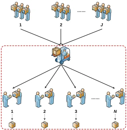
We model the supplier selection and order quantity allocation problem based on a two echelon inventory system. We assume the inventory decision is made by a single decision maker (i.e., centralized control), who wants to purchase a single product from a set of potential suppliers.
Figure3.1 depicts a serial supply chain system under considering of three levels, where raw
materials and products flow sequentially through the supply chain to satisfy the customer
demand. A single warehouse replenishes its inventory from a set ofS selected suppliers with
given lead times. It is assumed that all the suppliers in this identified set at level 1 satisfy the buyer’s qualitative criteria (service, delivery, maintenance, etc.) and the final decision will be made based on the item price, fixed ordering cost and the inventory cost regarding of
choosing the particular supplier. The warehouse then supplies the items to N independent
identical retailer, where demand occurs based on a Poisson process, and all stockouts are considered as backorders. Therefore, supplier selection and purchasing costs only occur at
the warehouse, while the product is transferred through the entire system, incurring costs like inventory costs, backorder cost, etc.
1 …… Level 2: Warehouse Level 1: Supplier 1 2 J 2 N …… Level 3: Retailer 3
Figure 3.1: Illustration of the multi-level supplier selection system
The above supply chain system is assumed to implement the continuous review (Q,
R) policy for the inventory system at the warehouse and the retailer. Hence, when the
demand occurs at the retailer, it is satisfied from the retailer’s available stock. Otherwise, the demand is backordered. Under this policy, the inventory position is checked continuously,
when it declines to the reorder point R, a batch size Q is ordered at the warehouse. The
of outstanding backorders. After an order is placed with the warehouse, an effective lead time
L takes place between placing the order and receiving it. After receiving the replenishment
order, the outstanding backorders at the retailer are immediately satisfied based on a first-come-first-serve (FCFS) policy.
For the warehouse, the retailer replenishment orders are satisfied if the on-hand inventory at the warehouse is greater than or equal to the retailer’s order size. That is, a partial
replenishment of an order at the warehouse is not allowed here. This is a reasonable
assumption when we consider a fixed order cost k connected to each transport from the
warehouse to the retailer. The inventory policy is followed as the same at the warehouse, i.e.,
the continuous review (Q, R) policy. We also adopt the widely-used two-echelon inventory
system assumption, that is the batch size and reorder point of the warehouse are the integral
number of that of the retailer (such as in (Axs¨ater,2003;Bodt and Graves,1985)). According
toChen and Zheng(1997), this integer-ratio order policy can facilitate quantity coordination among different facilities, and simplify packaging, transportation and stock counts. When the warehouse receives the replenishment order from the selected suppliers, any outstanding backorders are also fulfilled according to the FCFS policy.
In addition to determine the inventory policy for the warehouse and the retailer, we will not model any inventory process at the supplier. Instead, the decision maker should replenish the inventory for the warehouse and the retailer from different suppliers by performing a selection process so as to determine which supplier to be selected, the total expected quantity that are to be procured from the selected suppliers, and the frequency in which the orders are to be received. We assume that each supplier locates in different places, then prices, selection
costs, transportation costs, and replenishment lead times are diverse from each other. Define
S different suppliers, for each supplier, let Oj be the fixed ordering cost each time (i.e.,
selection cost, transportation cost, etc.), and pj be the price of one item from this supplier.
Moreover, µj and vj are respectively denoted as the mean and variance of transition time
from each supplier j to the warehouse, which is assumed to be known in advance. Supplier
j has limited maximum capacity Mj and a restriction of the minimum total order sizemj if
the supplier is selected. The objective of the proposed model is to coordinate the purchase, holding, backorder, and capacity in order to maximize the expected profit.
Before we introduce the mathematical model, we now define the notations that are used throughout the paper as the following:
Constants
S: number of suppliers
N: number of retailers
T: number of time span, in days
λr: demand rate at the retailer per day
L: replenishment lead time between the warehouse and the retailer, in days
pj: net purchase cost per unit from supplierj
h: holding cost per unit per day
b: backorder cost per unit per day
k: retailer’s fixed ordering cost per order
Oj: warehouse’s fixed ordering cost per order for supplierj
µj: mean replenishment lead time between supplierj and the warehouse, in
days
vj: variance of replenishment lead time between supplier j and the
warehouse, in days2
mj: minimum total order size of supplier j during T time units
Mj: maximum total order size of supplier j during T time units
Decision Variables
yj: binary variable, set to be 1 if supplierj is selected
xj: expected total ordering quantity from supplier j, in units
Qrj, Rrj: retailer’s order quantity and reorder point if supplier j is chosen,
in units
Qwj, Rwj: warehouse’s order quantity and reorder point if supplier j is
chosen, in units of retailer batches
Random Variables
tj: expected time to purchase orders from supplier j, in days
λw: demand rate at the warehouse per day
Ur: retailer’s retard time, in days
Irj(R, Q): expected on-hand inventory at retailer during the time supplier
Iwj(R, Q): expected on-hand inventory at warehouse during the time
supplierj is chosen, in units of retailer batches
Brj(R, Q): expected backorders at retailer during the time supplier j is
chosen, in units
Bwj(R, Q): expected backorders at warehouse during the time supplier j is
Chapter 4
Model Formulation
4.1
Mathematical Model
In this section, the model of supplier selection and order quantity allocation under
multi-echelon inventory system with stochastic Poisson demand is presented. Let xj be the
expected total ordering quantity from the supplier j and yj be a binary variable, where
yj = 1 means that supplier j is selected. Recall that each selected supplier j should satisfy
the capacity constraint, as a result, we may select different sets of suppliers when demand
rate at the retailer changes. The system is considered based on time span T. At this time,
we assume the demand rate at the retailer is constant. Moreover, at any moment, only one supplier is asked to provide the replenishment orders, i.e., no order splitting is considered every time the warehouse places the order. If there are multiple suppliers which are selected in the final decision, each supplier is assumed to serve the warehouse separately for some
purchase orders from supplier j. Thus, following one selected supplier (supplier a) that
finishes its service time (ta), the warehouse may place the order from another one (supplier
b) with some additional time (tb).
The no-order-splitting assumption represents the cases where the warehouse places orders from different suppliers one after another, and won’t order the same product from different suppliers at the same time. The reason to make this assumption is mainly due to the fact
that the different supplier lead time and ordering cost could require diverse (Q, R) policies
for both the warehouse and the retailer. However, it is untrackable and impractical to apply
different (Q, R) policies for different suppliers at the same moment. More specifically, to
apply the order-splitting assumption, the retailer may need to implement the same (Q, R)
policy no matter which supplier is selected. Moreover, it is still unclear that in which way (adopt this assumption or not) the system could be more efficient. Thus, we want to study the no-order-splitting situation first, and another model which violates this assumption will be considered in our future research.
The objective function of the proposed model consists of several parts to maximize the total expected profit. The first part is used to calculate total sale income. The second term corresponds to the purchasing cost incurred by all the units purchased from selected suppliers. The third part accounts for the total holding and backorder cost. The last term represents the fixed ordering cost for both echelons. The insights of the model is to examine the trade-offs among price, ordering, holding, and backorder costs to choose the best supplier(s) and decide the ordering policy. Based on the above discussed assumptions and variables, the
following mathematical model is designed: M aximize C = S X j=1 rxj− S X j=1 pjxj− S X j=1 tj[h(Irj+QrjIwj)+b(Brj+QrjBwj)]− S X j=1 ( xj QwjQrj Oj+ xj Qrj k). Subject to S X j=1 tj ≤T, (4.1) mjyj ≤xj ≤Mjyj j = 1, . . . , S, (4.2) xj =N λrtj j = 1, . . . , S, (4.3) Rrj ≥ −Qrj j = 1,· · · , S, (4.4) Rwj ≥ −Qwj j = 1,· · · , S, (4.5) Qrj, Qwj ≥0 j = 1,· · · , S, (4.6) Qrj, Rrj, Qwj&Rwj :Integers j = 1,· · · , S, (4.7) yj ∈ {0,1} j = 1, . . . , S. (4.8)
Constraint (4.1) ensures that the total expected time to purchase orders from all selected
suppliers should be no longer than the time span T. Constraint (4.2) defines the capacity
constraint for the selected suppliers. As for constraint (4.3), it ensures the expected ordering
quantity from supplier j should satisfy the expected demands at the retailer during its
can be shown that the optimal R satisfies R ≥ −Q. Therefore, it is assumed to satisfy in
equations (4.4) and (4.5), which can limit the computation efforts. Additionally, constrains
(4.6) and (4.7) are necessary, since there is no partial or fractional requests during the whole
process and the minimum allowable size is zero.
The mathematical model requires calculations of the expected inventory and backorder level for the warehouse and the retailer. We primarily elaborate the calculations in the following parts of this section.
4.2
The Retailer Inventory Analysis
Since the calculation for all the selected suppliers is identical, for notational ease, we ignore
the supplier’s subscriptj for the notations in this section. The following analysis is identical
for all the different supplier cases.
The retailer inventory position decreases with demand, and when the level reaches Rr,
an order of Qr is placed at the warehouse. Recall that in the steady state, the inventory
position is uniformly distributed over (Rr+ 1, Rr+ 2, · · ·,Rr+Qr). Under a (Q,R) policy,
the expected on-hand inventory for retailers is modeled as:
Ir =
Qr+ 1
2 +Rr+Br−E[Dr], (4.9)
whereE[Dr] is the retailer’s expected demand during the delay time. The delay time consists
the time between placement of an order by the retailer and the release of a batch by the
warehouse. The first part is denoted as L, which is assumed to be deterministic. While
the second part is usually called as the retard time, which is due entirely to the warehouse
stockout. We denote the retard time for the retailer as Ur. It is given as follows: the
number of arrival orders in the waiting system is precisely the warehouse’s backorders, and
the sojourn time is equal to the retailer’s retard time (Svoronos and Zipkin, 1988). Thus,
the expected retard time at the retailer is calculated as
E[Ur] = QrBw N λr , (4.10) then we have E[Dr] =λr(L+ QrBw N λr ). (4.11)
To simplify the calculation, as illustrated by (Hopp and Spearman, 2001), we adopt
normal approximation for the retailer’s demand during the delay time. It is worth to note that even though the demand process is Poisson process, the demand during the delay time for the retailer does not exactly follow the Poisson distribution, due to the variability of the retard time. In this paper, we ignore the variability of the retard time, and approximate the variance of the retailer’s expected demand during the delay time to be the same as its mean
Hence, using the normal approximation, expected backorders at the retailer Br can be computed as follows : Br = 1 Qr [β(Rr)−β(Rr+Qr)], (4.12) β(x) = σ 2 2 {(z 2+ 1)[1−Φ(z)]−zφ(z)}, (4.13) z = x−θ σ , (4.14)
where Φ and φ represent the cdf and pdf of the standard normal distribution, respectively.
Additionally, θ and σ are the mean and standard deviation of the demand during the delay
time. Note here for equation (4.13), it defines the continuous analog to the second-order loss
function β(x). Thus, substituting θ and σ in the above equations, Br can be computed in a
function based on the variables Qr, Rr, and Bw.
4.3
The Warehouse Inventory Analysis
To calculate the expected inventory level and backorder level at the warehouse, the demand process at the warehouse need to be analyzed first. Recall that the demand process at each
retailer is Poisson process, and the replenishment order for the warehouse is Qr each time.
However, the interval between any two orders is stochastic and depends on Qr. Hence,
the demand process at the warehouse is a superposition of the retailer’s ordering processes. Specifically, it is a superposition of independent renewal processes (i.e., the time between orders from each retailer are independent and identically distributed random variables),
(Deuermeyer and Schwarz,1981)). Therefore, under the assumption of identical retailers, it is straightforward to get the demand rate at the warehouse:
λw =
N λr
Qr
. (4.15)
When considering the multi-echelon problem, to determine the effective demand pattern at the upstream is always a difficult task. For this problem, it is almost impossible to find
an exact distribution for the demand process at the warehouse. However, Ganeshan (1999)
showed that whenN is greater than 20, the Poisson process is an excellent approximation for
the warehouse demand pattern. In our research,N is always a sufficient large number in each
scenario, so that each retailer’s order arrives approximately according to a Poisson process. This assumption is fairly reasonable, since for large retail corporation like Wal-Mart, the distribution center usually servers more than 20 stores.
Because of the independence of the superimpose process, given the mean and variance of
the warehouse replenishment lead time µand v, we can compute the mean and variance of
the warehouse demand during the replenishment lead time as
E[Dw] =µλw = N λrµ Qr , (4.16) V[Dw] =µλw+vλ2w = N λrµ Qr +N 2λ2 rµ2v Q2 r . (4.17)
Then we can obtain Iw similar to equation (4.9):
Iw =
Qw+ 1
2 +Rw+Bw−E[Dw]. (4.18)
Due to the assumption of Poisson demand process at the warehouse when N is sufficient
large, we also approximate the warehouse’s demand during the lead time as normal distribution. This is a reasonable approximation since this approximation improves as the rate of Poisson distribution increases, while the rate at the warehouse is sufficient large. This
approximation is also used in the literature, such as in (Al-Rifai and Rossetti, 2007). Then
equations (4.12) to (4.14) can also be adopted to calculate the expected backorder levelBw
at the warehouse. It is not hard to find out Bw is a function of Qw, Rw, and Qr.
4.4
Solution Procedure
The above multi-echelon supplier selection optimization model is a large-scale non-linear integer optimization problem. Considering the case of five potential suppliers, the model then may contain 30 integer decision variables, which takes a lot of computational time to solve. Moreover, the inventory analysis of each echelon requires to model and solve both echelons simultaneously. In order to model the warehouse, the retailer’s order batch size must be decided as a priori. On the other hand, the retailer’s calculation requires a known expected number of backorders at the warehouse. Thus, each echelon of the system is tightly connected with each other, and the model is difficult to solve in an efficient way.
Before we move forward, the following proposition gives some properties of the optimal decision.
Proposition 1. In an optimal solution, at most one supplier may not satisfy the following:
xj ∈ {0} S {mj, Mj}.
Proof. Assume that in an optimal solution, the suppliers aand b satisfy the condition ma<
xa < Ma and mb < xb < Mb respectively, so that the condition of Proposition 1 is violated.
Denote IBj =h(Irj +QrjIwj)/N λr+b(Brj +QrjBwj)/N λr, and Kj =Oj/QwjQrj+k/Qrj.
Then IBj and Kj are independent from xj. The objective function for C can be expressed
as PS
j=1rxj−
PS
j=1(pj+IBj +Kj)xj.
Without loss of generality, for suppliers a and b, we assume that pa +IBa +Ka <
pb+IBb+Kb. Also letϑ = min{xb−mb, Ma−xa}, x0a=xa+ϑ,x0b =xb−ϑ, andx0j =xj,
∀j 6=a, b. Then PS j=1(pj+IBj+Kj)x0j ≤ PS j=1(pj+IBj+Kj)xj. Since PS j=1x 0 j = PS j=1xj, (x01, x02, ..., x0S) would not violate constraint (4.1). Thus we have C0 ≥ C. This means (x01, x02, ..., x0S) is a better solution for this model, which violates the assumption. Continue
this process till at most one supplier supplies neither minimum nor maximum. This completes the proof.
As mentioned in the proof of the above proposition, the expected inventory and backorder level at the warehouse and the retailer are independent from the expected total ordering
quantity xj. This implies that the model can be solved with two decomposed levels: one
(Model 1) is to solve the optimal (Q,R) policy for each potential suppliers with the objective
choose the best suppliers with larger profit and allocate the expected order time for different suppliers. We now express the models as the following:
Model 1: Since the (Q, R) policy applied by different potential suppliers is independent
with each other, we formulate the optimization problem based on a single supplier j as
minimizing the total unit system cost, denoted as Ej, which includes inventory, backorder
and ordering cost as follows:
M inimize Ej =h(Irj +QrjIwj) +b(Brj +QrjBwj) + ( N λr QwjQrj Oj + N λr Qrj k). Subject to Rrj ≥ −Qrj, (4.19) Rwj ≥ −Qwj, (4.20) Qrj, Qwj ≥0, (4.21) Qrj, Rrj, Qwj&Rwj :Integers. (4.22)
Note in this model Irj, Iwj, Brj and Bwj can be formulated as the equations discussed in
section 4.2 and 4.3. For simplicity, we ignore those equations in this mathematical model.
Model 2: After achieving the minimized cost value Ej for each possible supplier, the
substituting Ej in the objective function as follows: M aximize C = S X j=1 rxj − S X j=1 pjxj − S X j=1 tjEj. Subject to S X j=1 tj ≤T, (4.23) mjyj ≤xj ≤Mjyj j = 1, . . . , S, (4.24) xj =N λrtj j = 1, . . . , S. (4.25)
Model 1 is a non-linear integer optimization model with two pairs of (Q, R) decision
variables to be solved. While model 2 is an integer programming model which is easy to solve. Apparently, this decomposition makes the multi-echelon supplier selection model to be solved in a more efficient way, since the sub-models provided above reduce the scale of the problem. Thus, we implement a solution procedure which can be summarized as the
following steps: (1) for each potential supplier j, solve Model 1 to achieve best (Qrj, Rrj)
and (Qwj, Rwj) values with the minimized values of Ej; (2) given the values of Ej for all
Chapter 5
Illustrative Example and Analysis
In this section, the numerical experiments are conducted with the proposed mathematical model. The model is coded in GAMS Integrated Development Environment, and solved by Knitro commercial package for mixed integer nonlinear model (Model 1) and Cplex for integer programming model (Model 2), in a desktop computer with an Intel Core(TM) 2 CPU(2.00 GHz) and 4GB RAM. The main purpose for the experiments in this section is to show the solvability and the effectiveness of the model and to demonstrate how to adopt the model for supplier selection decision making in different scenarios.
5.1
Parameter Setting
In this section, the system is simulated quarterly (i.e., T = 90), since the demand rate
usually doesn’t change a lot during a season. As mentioned earlier, the number of retailer is
Table 5.1: Parameter values assigned in the experiment
Parameter T N λr r h b k L
Value 90 20 10 100 1 3 100 1
to be chosen, which may locate in different regions of the world. As a result, we study the supplier selection problem based on one firm which consists of one warehouse and twenty identical retailers, and faces Poisson demands with the same arrival rate at the retailer. The
demand rate is set to be 10 units per day. Moreover, we set the product’s selling price r to
be 100. The unit holding cost and backorder cost for both the warehouse and the retailer are assumed to be 1 and 3 respectively. The fixed ordering cost from the warehouse to each retailer is considered as 100. Also the deterministic replenishment lead time from the warehouse to the retailer is set to be 1 (day). All the parameters are summarized in Table
5.1.
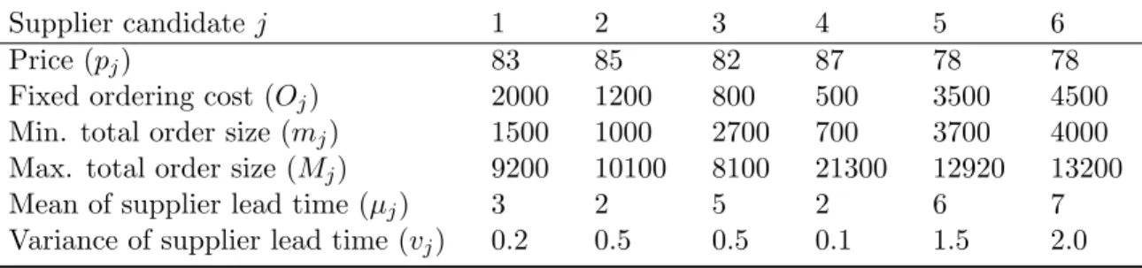
Table5.2shows additional data for each potential supplier. It is assumed all the suppliers
satisfy the buyer’s qualitative criteria, and own various purchasing price, fixed ordering cost, total expected order size constraint, and lead time. Two types of potential suppliers are considered: short-range suppliers (supplier 1, 2, 3, and 4) and long-distance suppliers
(supplier 5 and 6). As illustrated in Table 5.2, the long-distance suppliers charges less unit
purchasing cost, but requires more fixed ordering cost, and larger variability of the replenish lead time.
Table 5.2: Other parameter settings related to potential suppliers
Supplier candidate j 1 2 3 4 5 6
Price (pj) 83 85 82 87 78 78
Fixed ordering cost (Oj) 2000 1200 800 500 3500 4500
Min. total order size (mj) 1500 1000 2700 700 3700 4000
Max. total order size (Mj) 9200 10100 8100 21300 12920 13200
Mean of supplier lead time (µj) 3 2 5 2 6 7
Variance of supplier lead time (vj) 0.2 0.5 0.5 0.1 1.5 2.0
5.2
Results Analysis
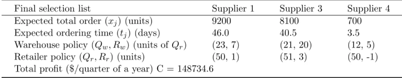
According to the above parameter settings, Table 5.3 displays the final selection decision.
The optimal inventory policy for each level and the selected supplier order allocation along with the total expected profit are also presented. Under such settings, supplier 1, 3 and 4 are selected. Recall that the decision to choose a supplier or not depends not only on the cost structures (i.e., unit cost, fixed ordering cost, inventory cost, and backorder cost), but also on the restriction for the minimum and maximum total expected order sizes. In this particular example, although the unit purchasing cost of the long-distance suppliers (supplier 5 and 6) is the least, nothing is ordered from them because of the high ordering cost and large variance of the replenishment lead time. Conversely, supplier 1 is selected due to its low lead time value and variation. Furthermore, supplier 4 is also chosen because of its low minimum total expected ordering quantity.
The model we built mainly focuses on the expected values for the selected suppliers. It does not intend to calculate the accurate quantity to make orders from the selected suppliers, but can indicate the priority to select suppliers. Since our model is based on stochastic
Table 5.3: Decision-making variables solution
Final selection list Supplier 1 Supplier 3 Supplier 4
Expected total order (xj) (units) 9200 8100 700
Expected ordering time (tj) (days) 46.0 40.5 3.5
Warehouse policy (Qw, Rw) (units of Qr) (23, 7) (21, 20) (12, 5)
Retailer policy (Qr, Rr) (units) (50, 1) (51, 3) (50, -1)
Total profit ($/quarter of a year) C = 148734.6
demands, in the real scenarios, the total order size and order time from selected suppliers
may not necessarily be the expected values calculated in Table5.3. For instance, according to
the results displayed in this table, supplier 1 and 3 own higher priority to be ordered since the expected order quantity reaches its upper limit of the capacity. In stochastic demand cases, we need to purchase from supplier 1 and 3 until the total order size reaches its maximum value, and the total order size from supplier 4 will depend on the real time demand. Hence,
x4 = 700 is only an expected value, and it implies that supplier 4 is the last choice to choose
when supplier 1 and 3 are available.
Considering the optimal (Q, R) policies of each selected supplier displayed in Table 5.3,
it is not surprising to find out that the retailer’s ordering quantity among different selected
suppliers are very similar. The main reason for this is that the replenishment quantity Qr
affects cycle stock (i.e., inventory that is held to avoid excessive replenishment costs), and the demand rate, retailer’s fixed ordering cost, and the replenishment lead time at the retailer are fixed no matter which supplier is chosen. Even the retard time may vary for different supplier, it only affects safety stock (i.e., inventory held to avoid stockouts), which determines
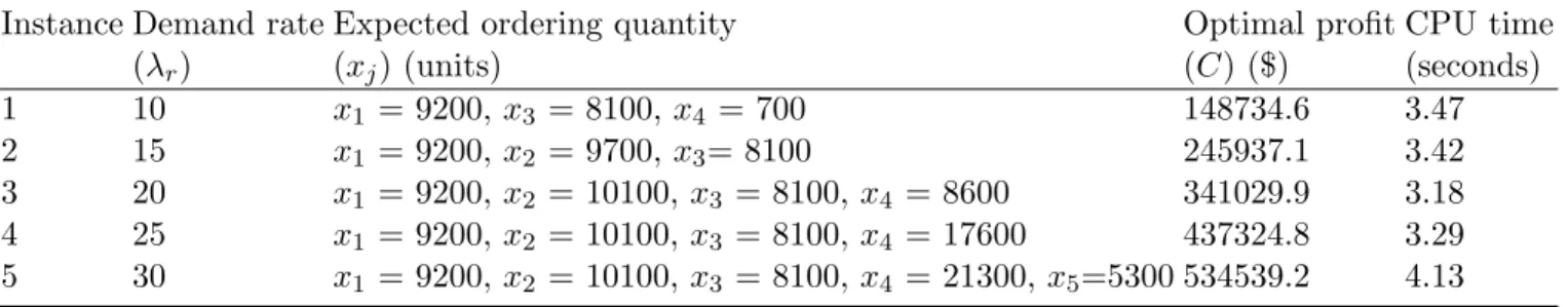
Table 5.4: The optimal policy and expected profit based on different demand rate instance
Instance Demand rate Expected ordering quantity Optimal profit CPU time
(λr) (xj) (units) (C) ($) (seconds) 1 10 x1 = 9200, x3 = 8100, x4 = 700 148734.6 3.47 2 15 x1 = 9200, x2 = 9700, x3= 8100 245937.1 3.42 3 20 x1 = 9200, x2 = 10100, x3 = 8100, x4 = 8600 341029.9 3.18 4 25 x1 = 9200, x2 = 10100, x3 = 8100, x4 = 17600 437324.8 3.29 5 30 x1 = 9200, x2 = 10100, x3 = 8100, x4 = 21300,x5=5300 534539.2 4.13
diverse (Q, R) strategies since they face different lead time and fixed ordering cost which
require to maintain different safety stock and cycle stock.
5.3
Demand Rate Analysis
To study the scenarios under different demand rate, we solve four additional problem
instances based on different value of λr, i.e., λr = 15, 20, 25, and 30. In this paragraph, all
the parameters remain the same as the settings in section5.1except for the retailer’s demand
rate. The demand rate value and the optimal policy for each instance are summarized in
Table 5.4. It is obvious that the expected profit increases due to the increase of demand. As
the demand rate increases, more suppliers are selected since the lower cost suppliers reach their maximum capacity. This implies that we should order up to capacities of the suppliers with lower costs when we selected at least two suppliers as supply partners. This also confirms the correctness of Proposition 1. Moreover, for all the instances, the long-distance suppliers own the least priority to be selected even though their unit price is smaller. This indicates that the demand rate doesn’t influence a lot to the cost structure of the suppliers, and the
long-distance suppliers here take more system costs which prevent them to be selected. The table also displays the CPU times to solve the problem for each case. The time is an average value based on 10 times run. For this case with six potential suppliers, it is possible to solve the model with the commercial software package in a short amount of time.
Table 5.5 displays the optimal inventory policy in different instances, which directly
corresponds to Table 5.4. Clearly, even if the same suppliers are selected in different
instances, their optimal inventory policies vary a lot. The retailer’s replenishment order
quantity and reorder point increase notably due to the increment of demand. This is
authentic since larger demand requires more cycle stock and safety stock to maintain low
cost. Based on the running instances, it can also be observed that the retailer’s order
quantity in each instance is almost the same among different selected suppliers. However, the retailer’s reorder point may vary among different supplier, especially for the selection of long-distance supplier (supplier 5) in instance 5. This is because long-distance supplier owns larger replenishment lead time variance which needs to hold more safety stock to avoid stockouts.
To clearly display the changes of (Q, R) policy at the warehouse for different instances,
Figure 5.1 is created to display the (Q, R) policy at the warehouse when supplier 1 and 3
is selected under different instances. Note in this figure, the values of order quantity and reorder point at the warehouse are based on the units of retailer’s order quantity. It is undoubted to observe the increasing trend in both the order quantity and reorder point due
to the increment of demands. It can also be inspected that Rw changes more considerable
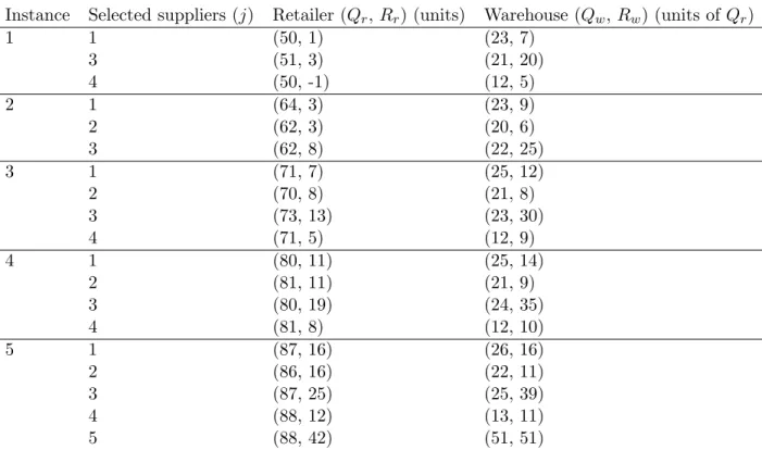
Table 5.5: The optimal inventory policy for selected suppliers in different demand rate instances
Instance Selected suppliers (j) Retailer (Qr,Rr) (units) Warehouse (Qw,Rw) (units of Qr)
1 1 (50, 1) (23, 7) 3 (51, 3) (21, 20) 4 (50, -1) (12, 5) 2 1 (64, 3) (23, 9) 2 (62, 3) (20, 6) 3 (62, 8) (22, 25) 3 1 (71, 7) (25, 12) 2 (70, 8) (21, 8) 3 (73, 13) (23, 30) 4 (71, 5) (12, 9) 4 1 (80, 11) (25, 14) 2 (81, 11) (21, 9) 3 (80, 19) (24, 35) 4 (81, 8) (12, 10) 5 1 (87, 16) (26, 16) 2 (86, 16) (22, 11) 3 (87, 25) (25, 39) 4 (88, 12) (13, 11) 5 (88, 42) (51, 51) 0 5 10 15 20 25 30 35 40 45 1 2 3 4 5 W a rehous e inv entory pol icy Instance
Supplier 1- Q Supplier 1- R Supplier 3- Q Supplier 3- R
Figure 5.1: Illustration of the trend for inventory policy at the warehouse when supplier 1 and 3 are selected under different instances
5.4
Long-distance Supplier Analysis
In this paragraph, we want to analyze the issue when selecting low-cost long-distant suppliers. In addition to high transportation cost (ordering cost), a long-distance supplier is often characterized by high delivery lead time and uncertainty. As shown in previous experiments, high lead time uncertainty results in large safety stock levels so that the expected inventory level will be high. To study the scenarios when a distant supplier should be selected and what quantity should be ordered, we conduct the experiments based on parameter changes
in long-distance supplier (price (pj), fixed ordering cost (Oj), mean supplier lead time (µj)
and variance of the delivery lead time (vj) are considered). According to the parameter
settings in section 5.1, we choose one long-distance supplier (supplier 5) to analyze, modify
one parameter once at a time (other parameters remain the same), and want to analyze
the impacts of the parameter on both expected ordering size xj (j = 5) and total expected
revenueC for different values of the demand rate instances (λr = 10, 15, and 20 are adopted
in this paragraph). Since supplier 5 is not chosen in the final decision of these instances, by doing so, we could examine the threshold value of each parameter to involve this distant supplier in our final selection.
We first study the scenario when the variance of delivery lead time changes. Figure 5.2
illustrates the changes of expected order quantity of supplier 5 and total expected profit when its delivery lead time variance varies from 0 to 1.4 under diverse demand rates. Observed in this figure, one can note that the expected total quantity purchased from the long-distance supplier decreases with the increasing lead time uncertainty. The figure shows that the
long-distance supplier should not be selected in some cases, especially when its lead time is highly uncertain. The right side of figure displays the total expected profit under the same experimental settings. Clearly, it can be observed that as the variance of long-distance supplier increases, the expected profit decrease. And when the variance is big enough, the lead time variance changes will not affect the total expected profit since this long-distance supplier will not even be chosen.
Keeping variance of lead time constant, Figure 5.3 demonstrates the changes of expected
order quantity and total expected profit when delivery lead time (µ5) varies from 4 to 5.8
under diverse demand rates. Note here the starting point value µ5 = 4 is set due to the
assumption of positive lead time (i.e., when mean and variance of normal distribution are separately 4 and 1.5, there is less than 0.05% probability that the lead time is negative). As
displayed in this figure, a similar trend can be observed as the one in Figure 5.2, which is
predicable. Comparing the total expected profit values in these two figures, one can note a lower lead time variance may let us earn more profit than a lower lead time mean. For
instance when demand rate is 20, a low delivery lead time where µ5 = 4 leads to almost
$800000 expected profit, however, a low lead time variance where v5 = 0.4 can result in a
profit more than that.
Keeping variance of lead time constant, it is demonstrated in Figure 5.3 the changes of
expected order quantity and total expected profit when delivery lead time (µ5) varies from
4 to 5.8 under diverse demand rates. Note here the starting point valueµ5 = 4 is set due to
the assumption of positive lead time (i.e., when mean and variance of normal distribution are separately 4 and 1.5, there is less than 0.05% probability that the lead time is negative).
0 2000 4000 6000 8000 10000 12000 14000 0 0.2 0.4 0.6 0.8 1 1.2 1.4 T ota l expec ted order qu antity (supplier 5)
Variance of the delivery lead time of the long-distance supplier Retailer's demand rate 10 Retailer's demand rate 15 Retailer's demand rate 20
0 200000 400000 600000 800000 1000000 1200000 0 0.2 0.4 0.6 0.8 1 1.2 1.4 T o ta l ex pected pr o fit
Variance of the delivery lead time of the long-distance supplier Retailer's demand rate 10 Retailer's demand rate 15 Retailer's demand rate 20
Figure 5.2: Illustration of the impact of delivery lead time variance for a long-distance supplier: total order quantity purchased from the distant supplier and the expected profit decrease with the increasing delivery lead time uncertainty
0 2000 4000 6000 8000 10000 12000 14000 4 4.3 4.6 4.9 5.2 5.5 5.8 T o ta l ex pect ed o rder qua nti ty (s uppl ier 5 )
Mean of the delivery lead time of the long-distance supplier
Retailer's demand rate 10 Retailer's demand rate 15 Retailer's demand rate 20
0 100000 200000 300000 400000 500000 600000 700000 800000 900000 4 4.3 4.6 4.9 5.2 5.5 5.8 T ota l expected pr ofi t
Mean of the delivery lead time of the long-distance supplier Retailer's demand rate 10 Retailer's demand rate 15 Retailer's demand rate 20
Figure 5.3: Illustration of the impact of mean delivery lead time for a long-distance supplier: total order quantity purchased from the distant supplier and the expected profit decrease with the increasing mean delivery lead time
As displayed in this figure, a similar trend can be observed as the one in Figure 5.2, which is predicable. Comparing the total expected profit values in these two figures, one can note a lower lead time variance may let us earn more profit than a lower lead time mean. For
instance when demand rate is 20, a low delivery lead time where µ5 = 4 leads to almost
$800,000 expected profit, however, a low lead time variance where v5 = 0.4 can result in a
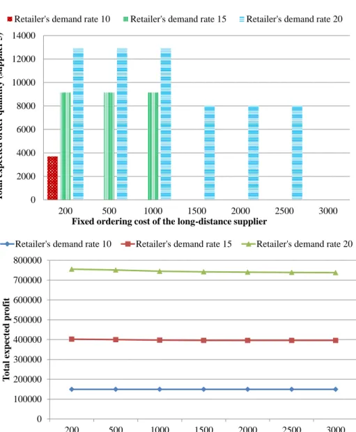
0 2000 4000 6000 8000 10000 12000 14000 200 500 1000 1500 2000 2500 3000 T o ta l ex pected o rder quanti ty (s uppli er 5 )
Fixed ordering cost of the long-distance supplier
Retailer's demand rate 10 Retailer's demand rate 15 Retailer's demand rate 20
0 100000 200000 300000 400000 500000 600000 700000 800000 200 500 1000 1500 2000 2500 3000 T o ta l ex pect ed pr o fi t
Fixed ordering cost of the long-distance supplier
Retailer's demand rate 10 Retailer's demand rate 15 Retailer's demand rate 20
Figure 5.4: Illustration of the impact of fixed ordering cost for a long-distance supplier: total order quantity purchased from the distant supplier and the expected profit decrease with the increasing fixed ordering cost
0 2000 4000 6000 8000 10000 12000 14000 73 74 75 76 77 T o ta l expected o rder quanti ty (s uppli er 5 )
Unit price of the long-distance supplier
Retailer's demand rate 10 Retailer's demand rate 15 Retailer's demand rate 20
0 100000 200000 300000 400000 500000 600000 700000 800000 900000 1000000 73 74 75 76 77 T o ta l ex pected pr o fi t
Unit price of the long-distance supplier
Retailer's demand rate 10 Retailer's demand rate 15 Retailer's demand rate 20
Figure 5.5: Illustration of the impact of unit price for a long-distance supplier: total order quantity purchased from the distant supplier and the expected profit decrease with the increasing unit price
Chapter 6
Conclusions
In this paper, we study a supplier selection and order allocation problem in a multi-echelon system under stochastic demand, where a buyer firm that consists of one warehouse and
N identical retailers focuses its attention to analyze both supplier selection decisions and
inventory control policies to optimize the entire system. Capacity, ordering cost, unit price, holding and backorder cost are considered as the criteria for the supplier selection. A mixed integer non-linear programming (MINLP) model is proposed to select the best suppliers and determine a coordinated replenishment inventory policy at each echelon of the supply chain so that the total expected profit is maximized. To solve the model more efficiently, we decompose the mathematical model into two sub-models. Our experiments demonstrate the solvability and the effectiveness of the model. Moreover, we have been interested in some issues regarding the selection of the long-distance supplier. Thus, some sensitivity analysis for the long-distance supplier is also conducted.
There are two limitations for the current work in this paper. First, we have adopted the no-order-splitting assumption, which requires ordering from a certain supplier for some continues time span. The reason to make this assumption is mainly due to the different
(Q, R) inventory policy adopted at both the warehouse and retailers for different selected
suppliers. However, observed in our experimental examples in Section 5.3, similar (Q, R)
polices are assigned to the retailer for different suppliers. This implies that it is possible to apply the order splitting model at the warehouse. Thus, future work may focus on extending order splitting model at the warehouse and the same ordering policy for the retailer. Second, to implement the stochastic demand assumption, we mainly focus on calculating the expected values of the total ordering size and the time. The intention to use these expected values is not for signing the contract and ordering the computed amount from the selected suppliers, but for deciding the priorities to select suppliers and estimating the size and time to order from each supplier. Our model offers more insights to choose suppliers and allocate orders among the suppliers when considering the integration of both the supplier selection and inventory control problems in the multi-echelon system under stochastic demand.
There are several directions for the future work. First, as we mentioned above, the
order-splitting model is a good direction to work on. Second, in this paper we assume the (Q, R)
continuous review policy. Future work may consider periodic review system. Moreover, our model can be extended to consider multiple product and joint replenishment costs. Finally, since the supplier selection is a typical multi-criteria decision problem, this work could be extended to multi-objective models where the trade-offs associated with these criteria can be analyzed.
Aissaoui, N., Haouari, M., and Hassini, E. (2007). Supplier selection and order lot sizing
modeling: A review. Computers & Operations Research, 34(12):3516–3540. 1, 2, 6
Al-Rifai, M. H. and Rossetti, M. D. (2007). An efficient heuristic optimization algorithm
for a two-echelon (r, q) inventory system. International Journal of Production Economics,
109(1-2):195–213. 23
Amid, A., Ghodsypour, S., and OBrien, C. (2009). A weighted additive fuzzy multiobjective
model for the supplier selection problem under price breaks in a supply chain.International
Journal of Production Economics, 121(2):323–332. 8
Awasthi, A., Chauhan, S., Goyal, S., and Proth, J.-M. (2009). Supplier selection problem for
a single manufacturing unit under stochastic demand.International Journal of Production
Economics, 117(1):229–233. 8
Axs¨ater, S. (2003). Supply chain operations: serial and distribution inventory systems. In
A.G. de Kok and S.C. Graves, Eds., Handbooks in Operations Research and Management Science, volume 11, pages 525–559. 12
Bodt, M. A. D. and Graves, S. C. (1985). Continuous-review policies for a multi-echelon
inventory problem with stochastic demand. Management Science, 31(10):1286–1299. 12
Chen, F. and Zheng, Y.-S. (1997). One-warehouse multiretailer systems with centralized
stock information. Operations Research, 45(2):275–287. 12
de Boer, L., Labro, E., and Morlacchi, P. (2001). A review of methods supporting supplier
Degraeve, Z., Labro, E., and Roodhooft, F. (2000). An evaluation of vendor selection models
from a total cost of ownership perspective. European Journal of Operational Research,
125(1):34–58. 5
Demirtas, E. A. and Ustun, O. (2009). Analytic network process and multi-period goal
programming integration in purchasing decisions. Computers & Industrial Engineering,
56(2):677–690. 7, 8
Deuermeyer, B. L. and Schwarz, L. B. (1981). A model for the analysis of system service
level in warehouse retailer distribution systems: The identical retailer case. TIMS Studies
in the Management Science, 16:163–193. 22
Ganeshan, R. (1999). Managing supply chain inventories: A multiple retailer, one warehouse,
multiple supplier model. International Journal of Production Economics, 59(1-3):341–354.
22
Ghodsypour, S. and O’Brien, C. (1998). A decision support system for supplier selection
using an integrated analytic hierarchy process and linear programming. International
Journal of Production Economics, 56-57:199–212. 6
Hammami, R., Frein, Y., and Hadj-Alouane, A. B. (2012). An international supplier selection
model with inventory and transportation management decisions. Flexible Services and
Haq, A. N. and Kannan, G. (2006). Design of an integrated supplier selection and multi-echelon distribution inventory model in a built-to-order supply chain environment.
International Journal of Production Research, 44(10):1963–1985. 8
Hayes, R. H., Pisano, G. P., Upton, D. M., and Wheelwright, S. C. (2005). Operations,
strategy, and technology. NewYork:Wiley. 1
Ho, W., Xu, X., and Dey, P. K. (2010). Multi-criteria decision making approaches for supplier
evaluation and selection: A literature review. European Journal of Operational Research,
202(1):16–24. 5
Hong, G. H., Park, S. C., Jang, D. S., and Rho, H. M. (2005). An effective supplier
selection method for constructing a competitive supply-relationship. Expert Systems with
Applications, 28(4):629–639. 7
Hopp, W. and Spearman, M. (2001). Factory Physics. McGraw-Hill/Irwin, 2nd edition. 20
Jayaraman, V., Srivastava, R., and Benton, W. C. (1999). Supplier selection and order
quantity allocation: A comprehensive model. Journal of Supply Chain Management,
35(2):50–58. 1
Kasilingam, R. G. and Lee, C. P. (1996). Selection of vendors - a mixed-integer programming
approach. Computers & Industrial Engineering, 31(1):347–350. 6
Liao, Z. and Rittscher, J. (2007). A multi-objective supplier selection model under stochastic
Mendoza, A. and Ventura, J. A. (2010). A serial inventory system with supplier selection and
order quantity allocation. European Journal of Operational Research, 207(3):1304–1315.
2, 8
Narasimhan, R., Talluri, S., and Mahapatra, S. K. (2006). Multiproduct, multicriteria model
for supplier selection with product life-cycle considerations. Decision Sciences, 37(4):577–
603. 7
Ng, W. L. (2008). An efficient and simple model for multiple criteria supplier selection
problem. European Journal of Operational Research, 186(3):1059–1067. 6
Svoronos, A. and Zipkin, P. (1988). Estimating the performance of multi-level inventory
systems. Operations Research, 36(1):57–72. 20
Talluri, S. (2002). A buyer-seller game model for selection and negotiation of purchasing
bids. European Journal of Operational Research, 143(1):171–180. 6
Talluri, S. and Narasimhan, R. (2003). Vendor evaluation with performance variability: A
max-min approach. European Journal of Operational Research, 146(3):543–552. 6
Wadhwa, V. and Ravindran, A. R. (2007). Vendor selection in outsourcing. Computers &
Operations Research, 34(12):3725–3737. 1
Weber, C. A., Current, J. R., and Benton, W. (1991). Vendor selection criteria and methods.
Xia, W. and Wu, Z. (2007). Supplier selection with multiple criteria in volume discount
environments. Omega, 35(5):494–504. 7
Yang, P., Wee, H., Pai, S., and Tseng, Y. (2011). Solving a stochastic demand multi-product supplier selection model with service level and budget constraints using genetic algorithm.
Expert Systems with Applications, 38(12):14773–14777. 8
Zhang, J. and Zhang, M. (2011). Supplier selection and purchase problem with fixed cost and
constrained order quantities under stochastic demand.International Journal of Production
Vita
Cong Guo was born in Nantong, China. He graduated in 2009 with a Bachelor’s degree
in Industrial Engineering from Huazhong University of Science and Technology. In the
fall of 2009, he joined Dr. Xueping Li’s group as a graduate assistant at the Department of Industrial and Systems Engineering of University of Tennessee, Knoxville. He plans to achieve a concurrent Master of Science degree in Industrial Engineering in August 2013.