On the Performance of some Poisson Ridge Regression Estimators

(1)

Florida International University

FIU Digital Commons

FIU Electronic Theses and Dissertations

University Graduate School

3-28-2018

On the Performance of some Poisson Ridge

Regression Estimators

Cynthia Zaldivar

Florida International University

, [email protected]

DOI:

10.25148/etd.FIDC006538

Follow this and additional works at:

https://digitalcommons.fiu.edu/etd

Part of the

Applied Statistics Commons

,

Multivariate Analysis Commons

,

Other Statistics and

Probability Commons

,

Statistical Methodology Commons

,

Statistical Models Commons

,

Statistical

Theory Commons

, and the

Theory and Algorithms Commons

This work is brought to you for free and open access by the University Graduate School at FIU Digital Commons. It has been accepted for inclusion in FIU Electronic Theses and Dissertations by an authorized administrator of FIU Digital Commons. For more information, please [email protected].

Recommended Citation

Zaldivar, Cynthia, "On the Performance of some Poisson Ridge Regression Estimators" (2018).FIU Electronic Theses and Dissertations. 3669.

(2)

FLORIDA INTERNATIONAL UNIVERSITY

Miami, Florida

ON THE PERFORMANCE OF SOME POISSON RIDGE REGRESSION

ESTIMATORS

A thesis submitted in partial fulfillment of the

requirements for the degree of

MASTER OF SCIENCE

in

STATISTICS

by

Cynthia Zaldivar

2018

(3)

To: Dean Michael R. Heithaus

College of Arts, Sciences and Education

This thesis, written by Cynthia Zaldivar, and entitled On the Performance of Some

Pois-son Ridge Regression Estimators, having been approved in respect to style and

intellec-tual content, is referred to you for judgment.

We have read this thesis and recommend that it be approved.

Wensong Wu

Florence George

B. M. Golam Kibria, Major Professor

Date of Defense: March 28, 2018

The thesis of Cynthia Zaldivar is approved.

Dean Michael R. Heithaus

College of Arts, Sciences and Education

Andr´es G. Gil

Vice President for Research and Economic Development

and Dean of the University Graduate School

(4)

ACKNOWLEDGEMENTS

I would like to thank the members of my committee — Dr. Florence George and Dr.

Wensong Wu — for their support and advice regarding this thesis. I would also like to

thank Kristofer Månsson of J¨onk¨oping University for his help with the Monte Carlo

sim-ulation, finding data for the applications section, and answering any questions I had.

Fi-nally, I would like to thank my major professor, Dr. B. M. Golam Kibria, for his constant

support throughout the process. His expertise on the subject matter has been crucial to the

research.

(5)

ABSTRACT OF THE THESIS

On the Performance of Some Poisson Ridge Regression Estimators

by

Cynthia Zaldivar

Florida International University, 2018

Miami, Florida

Professor B. M. Golam Kibria, Major Professor

Multiple regression models play an important role in analyzing and making

predic-tions about data. Prediction accuracy becomes lower when two or more explanatory

vari-ables in the model are highly correlated. One solution is to use ridge regression. The

pur-pose of this thesis is to study the performance of available ridge regression estimators for

Poisson regression models in the presence of moderately to highly correlated variables.

As performance criteria, we use mean square error (MSE), mean absolute

percent-age error (MAPE), and percentpercent-age of times the maximum likelihood (ML) estimator

pro-duces a higher MSE than the ridge regression estimator.

A Monte Carlo simulation study was conducted to compare performance of the

es-timators under three experimental conditions: correlation, sample size, and intercept. It

is evident from simulation results that all ridge estimators performed better than the ML

estimator. We proposed new estimators based on the results, which performed very well

compared to the original estimators. Finally, the estimators are illustrated using data on

recreational habits.

(6)

TABLE OF CONTENTS

CHAPTER

PAGE

1

INTRODUCTION

1

1.1

Literature Review . . . .

1

1.2

Objective of the Thesis . . . .

3

2

METHODOLOGY

4

2.1

Poisson Ridge Regression . . . .

4

2.2

Estimating the k Parameter . . . .

6

2.3

k Estimators Used . . . .

7

2.4

Criteria for Good Estimators . . . 13

2.5

Inducing Outliers . . . 13

3

THE MONTE CARLO SIMULATION

15

3.1

Simulation Technique . . . 15

3.2

Simulation Results

. . . 16

3.3

Performance as a Function of

β

0

. . . 20

3.4

ρ

. . . 20

3.5

n

. . . 20

3.6

Best Performing Estimators . . . 20

3.7

Proposed New Estimators . . . 21

3.8

Performance of New Estimators

. . . 21

4

APPLICATION

25

5

SUMMARY AND CONCLUDING REMARKS

28

REFERENCES

30

(7)

LIST OF TABLES

TABLE

PAGE

3.1

Poisson Regression Simulation Results, P

=

4, n

=

35, Correlation(

ρ

)

=

.

85

. . . 17

3.2

=

4, n

=

600,

ρ

=

.

85

. . . 18

3.3

MSE Ratios (10% Outliers), P

=

4, n

=

35

. . . 19

3.4

Poisson Regression Simulation Results (New Estimators), P

=

4, n

=

35,

ρ

=

.

85

. . . 22

3.5

=

4, n

=

600,

ρ

=

.

85 . . . 23

4.1

VIF for each regressor

. . . 26

4.2

MSE for Each k Estimator - Recreation Data

. . . 26

4.3

Significance of Coe

ffi

cients from MLE and Selected New Estimators

. . . 26

4.4

Estimated Regression Coe

ffi

cients for Each Model

. . . 27

A1

=

4, n

=

35,

ρ

=

.

90 . . . 35

A2

=

4, n

=

35,

ρ

=

.

95 . . . 36

A3

=

4, n

=

35,

ρ

=

.

99 . . . 37

A4

=

4, n

=

600,

ρ

=

.

90 . . . 38

A5

=

4, n

=

600,

ρ

=

.

95 . . . 39

A6

=

4, n

=

600,

ρ

=

.

99 . . . 40

A7

=

4, n

=

35,

ρ

=

.

90 41

A8

Poisson Regression Simulation Results (New Estimators), P

=

4, n

=

35,

ρ

=

.

95 42

A9

=

4, n

=

35,

ρ

=

.

99 43

A10 Poisson Regression Simulation Results (New Estimators), P

=

4, n

=

600,

ρ

=

.

90 . . . 44

=

4, n

=

600,

ρ

=

.

95 . . . 45

=

4, n

=

600,

ρ

=

.

99 . . . 46

(8)

LIST OF FIGURES

FIGURE

PAGE

3.1

MSE for each k estimator,

n

=

35,

ρ

=

.

85 . . . 16

3.2

Estimators with Smallest MSE (n

=

35,

ρ

=

.

85,

β

0

=

−

1)

. . . 24

A1

MSE for each k estimator,

ρ

=

.

90 . . . 33

A2

MSE for each k estimator,

ρ

=

.

95 . . . 34

(9)

CHAPTER 1

INTRODUCTION

1.1

Literature Review

When any pair of independent variables are highly correlated, the corresponding

regres-sion coe

ffi

cients will have large standard errors, which means that the regression coe

ffi

-cients are unstable. When two independent variables are highly correlated, they are not

orthogonal, that is the regressors have a near linear relation. In such a situation, the

coef-ficients are less likely to be statistically significant. Inferences made using such a model

will not be correct. This type of situation is referred to as multicollinearity. (Allen, 1997)

Two methods of dealing with multicollinearity are collecting more data and model

respecification. While collecting more data may be the best way to correct

multicollinear-ity, it is not always possible to collect additional data. There are often financial constraints

which render the solution impossible. Finances aside, the process, individuals, or items

being studied may no longer be accessible for sampling. Collecting more data may not

solve the issue of multicollinearity if the problem arises from limitations of the model

or population. If multicollinearity is caused by some characteristic of the model, such as

the presence of two highly correlated variables, model respecification may help alleviate

the issue. The discovery and implementation of a simple function, such as

x

=

x

1

/

x

2 or

x

=

x

1

x

2 may aid the issue while preserving the information gained from the regressors.

One e

ff

ective method of dealing with multicollinearity is elimination of any highly

cor-related variables. While this kind of brute force method may totally remove the issue, the

information gained from any removed regressors will be lost. The loss of information can

be an unacceptable consequence to many researchers. (Montgomery, 2012)

(10)

The widely used method of dealing with multicollinearity is through the use of ridge

regression, in which regression coe

ffi

cients are calculated as such:

ˆ

βR

(

k

)

=

(

X

0

X

+

kI

)

−1

X

0

y

.

(1.1)

Here X is an

nx

(

p

+

1) matrix, p being the number of independent variables used in

the model.For values

k

≥

0 the mean square error (MSE) is smaller than that of the least

squares estimator:

ˆ

β

=

(

X

0

X

)

−1

X

0

y

.

(1.2)

The ridge regression method of dealing with multicollinearity was originally

pro-posed by Hoerl and Kennard (1970). Many researchers have propro-posed estimates for k,

including Lawless and Wang (1976), Kibria (2003), Alkhamisi and Shukur (2008), Kibria

and Mu˜niz (2009), Kibria and Banik (2016), and Asar and Genc¸ (2017), among others.

There has been limited research on ridge regression using non-Gaussian regression

models, such as the Poisson regression model. Månsson and Shukur (2011) evaluated

the performance of several k estimators for Poisson ridge regression using Monte Carlo

simulations. The present thesis expands on that study by evaluating more k estimators and

proposing some new k estimators for Poisson ridge regression models.

The Poisson regression model has a large amount of applications, especially in

eco-nomics. A Poisson model is useful when the response variable includes countable,

inde-pendent events, such as the total number of car accidents per week on a specific highway,

the number of calls received per minute at a call center, or number of credit defaults per

year (Greene, 2012). Further applications will be discussed in Section 4 of this thesis.

(11)

1.2

Objective of the Thesis

The problem of estimating k is the subject of many research papers and has not been

solved yet. The di

ff

erent methods proposed in research each have advantages and

disad-vantages. It is necessary to compare di

ff

erent estimators under di

ff

erent error distributions

under the same conditions. The purpose of this research is to compare popular ridge

pa-rameter estimators using the following criteria:

1. Smallest mean squared error (MSE)

2. Mean absolute percentage error (MAPE)

3. Performance of ridge regression estimator compared to the least squares estimator,

in terms of the percentage of times in simulation that the ridge regression estimator

produces a lower MSE than the least squares estimator.

The present research extends Poisson Ridge Regression (PRR) research by

Måns-son and Shukur (2011). Ridge regression estimators for PoisMåns-son regression models will

be compared to the maximum likelihood estimation (MLE) method using Monte Carlo

simulations.

The organization of the thesis is as follows. We define di

ff

erent types of ridge

re-gression estimators of k in Chapter 2. A Monte Carlo simulation study has been

con-ducted in Chapter 3. In Chapter 4, the empirical application of the Poisson ridge

regres-sion is presented. The summary and concluding remarks are given in Chapter 5.

(12)

CHAPTER 2

METHODOLOGY

2.1

Poisson Ridge Regression

In Poisson regression, it is standard to cross-section data in applications of n independent

observations. The

i

th

observation is (

y

i

,

x

i

). Here

y

i

, the dependent variable, represents

the number of occurrences of the event of interest and

x

0

i

=

n

x

1i,

x

2i

, ...,

x

pi

o

is a vector of

p linearly independent regressors that are thought to determine

y

i

.

y

i

given

x

i

is Poisson

distributed, with the density function:

f

(

y

i

|

x

i

)

=

e

−µi

µ

yi

i

y

i

!

,

y

i

=

0

,

1

,

2

, ...

.

(2.1)

The mean parameter, which represents the average rate of occurrence of the event of

inter-est, is calculated as:

µi

=

e

x0_iβ

,

(2.2)

where

β

is a vector of parameters from the regression model.

The Maximum Likelihood Estimator (MLE) for

β

is found using the iterative weighted

least square (IWLS) algorithm:

ˆ

βMLE

=

(

X

0

W X

ˆ

)

−1

X

0

W

ˆ

z

ˆ

,

(2.3)

where ˆ

W

=

diag

( ˆ

µi

),

µi

ˆ

=

e

xiβˆ

,

and ˆ

z

=

log

( ˆ

µi

)

+

y

i

−

µi

ˆ

µi

.

The Poisson ridge regression estimator is calculated as:

ˆ

(13)

where

U

=

(

X

0

W X

ˆ

+

kI

)

−1

X

0

W X

ˆ

The MSE of ˆ

βR

(

k

) can be calculated as follows:

MS E

βR

ˆ

(

k

)

=

MS E

U

βMLE

ˆ

=

E

U

βMLE

ˆ

−

β

0

U

βMLE

ˆ

−

β

=

E

β

ˆ

0

MLE

U

0

U

βMLE

ˆ

−

E

β

0

U

βMLE

ˆ

−

E

β

ˆ

0

MLE

U

0

β

+

E

(

β

0

β

)

=

E

β

ˆ

0_MLE

U

0

U

βMLE

ˆ

−

E

β

0

U

0

U

βMLE

ˆ

−

E

β

ˆ

0_MLE

U

0

U

β

+

E

β

ˆ

0_MLE

U

0

U

β

+

E

(

β

0

U

0

U

β

)

−

E

(

β

0

U

0

U

β

)

+

E

β

0

U

0

U

βMLE

ˆ

−

E

β

0

U

βMLE

ˆ

−

E

β

ˆ

0_MLE

U

0

β

+

E

(

β

0

β

)

(2.5)

Lee and Silvapulle (1988) found that, for large values of

n

, the distribution of ˆ

βMLE

is

ˆ

βMLE

∼

N

β,

X

0

W X

ˆ

−1

. Then:

MS E

βR

ˆ

(

k

)

=

E

h

βMLE

ˆ

−

β

0

U

0

U

βMLE

ˆ

−

β

i

−

β

0

U

0

U

β

+

β

0

U

0

U

β

+

β

0

U

0

U

β

−

β

0

U

β

−

β

0

U

0

β

+

β

0

β

=

E

h

βMLE

ˆ

−

β

0

U

0

U

βMLE

ˆ

−

β

i

+

β

0

U

−

I

p

0

U

−

I

p

β

=

E

h

tr

h

βMLE

ˆ

−

β

0

U

0

U

βMLE

ˆ

−

β

ii

+

β

0

U

−

I

p

0

U

−

I

p

β

=

E

h

tr

h

U

βMLE

ˆ

−

β

βMLE

ˆ

−

β

0

U

0

ii

+

β

0

U

−

I

p

0

U

−

I

p

β

=

tr

h

U E

h

βMLE

ˆ

−

β

βMLE

ˆ

−

β

0

i

U

0

i

+

β

0

U

−

I

p

0

U

−

I

p

β

=

tr

U

X

0

W X

ˆ

−1

U

0

+

β

0

U

−

I

p

0

U

−

I

p

β

=

tr

h

X

0

W X

ˆ

+

kI

p

)

−2

X

0

W X

ˆ

i

+

β

0

−

k

X

0

W X

ˆ

+

kI

p

−1

0

−

k

X

0

W X

ˆ

+

kI

p

−1

β

=

tr

X

0

W X

ˆ

+

kI

p

−2

X

0

W X

ˆ

+

β

0

k

2

X

0

W X

ˆ

+

kI

p

−2

β

(14)

Let

C

=

X

0

W X

ˆ

and

Λ =

diag

(

λ

1

, λ

2

, ..., λp

) be the eigenvalues of C. Suppose there exists

an orthogonal matrix D such that

D

0

CD

= Λ

, then:

=

tr

X

0

W X

ˆ

+

kI

p

−2

X

0

W X

ˆ

+

β

0

k

2

X

0

W X

ˆ

+

kI

p

−2

β

=

tr

DD

0

X

0

W X

ˆ

+

kI

p

−1

DD

0

X

0

W X

ˆ

+

kI

p

−1

DD

0

X

0

W X

ˆ

+

k

2

(

D

β

)

0

D

0

X

0

W XD

ˆ

+

kDD

0

−2

(

D

β

)

=

tr

D

0

X

0

W X

ˆ

+

kI

p

−1

DD

0

X

0

W X

ˆ

+

kI

p

−1

DD

0

X

0

W XD

ˆ

+

k

2 p

P

i=1

α

2 i

(

λi

+

k

)

2

=

tr

D

0

X

0

W XD

ˆ

+

kI

p

−1

D

0

X

0

W XD

ˆ

+

kI

p

−1

D

0

X

0

W XD

ˆ

+

k

2 p

P

i=1

α

2 i

(

λi

+

k

)

2

=

tr

Λ +

kI

p

−1

Λ +

kI

p

−1

Λ

+

k

2 p

P

i=1

α

2 i

(

λi

+

k

)

2

=

P

p i=1

λi

(

λi

+

k

)

2

+

k

2

P

p i=1

α

2 i

(

λi

+

k

)

2

=

Var

ˆ

β

R

(

k

)

+

Bias

β

ˆ

R

(

k

)

2

(2.6)

where

λi

is the

i

th

eigenvalue of C and

α

=

D

β

Månsson (2011)

2.2

Estimating the k Parameter

Let ˆ

α

(

k

)

=

(

X

∗0

X

∗

+

kI

)

−1

X

∗0

y

,

(2.7)

where

k

=

diag

(

k

1

,

k

1

, ...,

k

p

),

k

i

>

0,

MS E

( ˆ

α

(ˆ

k

))

=

p

P

i=1

λi

(

λi

+

k

ˆ

i

)

2

+

P

p i=1

ˆ

k

2 i

α

ˆ

2 i

(

λi

+

k

ˆ

i

)

2

(2.8)

The value of which

k

i

minimizes

MS E

( ˆ

α

(ˆ

k

)) is:

ˆ

k

i

=

1

ˆ

α

2 i

(15)

2.3

k Estimators Used

This thesis will analyze the performance of 50 di

ff

erent k estimators. The k estimators

used in this thesis are summarized below.

The first two k are from Hoerl and Kennard (1970):

HK

=

k

ˆ

HK

=

1

ˆ

α

2 max

(2.10)

HK

2

=

K

ˆ

HK2

=

1

P

p i=1

α

ˆ

2 i

(2.11)

A di

ff

erent estimator, produced by taking the harmonic mean of ˆ

k

i

was suggested by

Ho-erl et al. (1975):

HK

B

=

k

ˆ

HK B

=

p

P

i=1

ˆ

α

2 i

=

p

ˆ

α

0

α

ˆ

(2.12)

The next k estimator was proposed by Lawless and Wang (1976):

ˆ

k

LWi

=

1

λi

α

ˆ

2_i

(2.13)

and suggest taking the harmonic mean of (2.13):

LW

=

k

ˆ

LW

=

p

P

i=1

λi

α

ˆ

2_i

=

p

ˆ

α

0

X

0

X

α

ˆ

(2.14)

(16)

HS L

=

k

ˆ

HS L

=

p

P

i=1

(

λi

αi

ˆ

)

2 p

P

i=1

λi

α

ˆ

2 i

!

2

(2.15)

The next three k estimators, proposed by Kibria (2003), take the arithmetic mean,

geo-metric mean, and median of the ridge estimator ˆ

k

i

:

AM

=

k

ˆ

AM

=

1

p

P

i=1

1

ˆ

α

2 i

(2.16)

GM

=

k

ˆ

GM

=

1

(

p

Q

i=1

ˆ

α

2 i

)

1 /p

(2.17)

Med

=

k

ˆ

Med

=

Median

1

ˆ

α

2 i

!

(2.18)

Khalaf and Shukur (2005) suggested the following k estimator:

KS

=

K

ˆ

KS

=

λmax

(

n

−

p

)

+

λmax

α

ˆ

2

max

(2.19)

Alkhamisi et al. (2006) proposed the following:

KS

A

=

K

ˆ

_ArithKS

=

1

p

P

p i=1

λi

(

n

−

p

)

+

λi

α

ˆ

2_i

!

(2.20)

KS

Max

=

K

ˆ

_MaxKS

=

Max

(

λi

(

n

−

p

)

+

λi

α

ˆ

2

i

)

(2.21)

KS

Med

=

K

ˆ

_MedKS

=

Median

(

λi

(

n

−

p

)

+

λi

α

ˆ

2

i

)

(2.22)

(17)

mean of

λi

(

n

−

p

)

+

λi

α

ˆ

2 i

!

,

K M

1

=

K

ˆ

GMKS

=

K

ˆ

K M1

=

Q

p i=1

λi

(

n

−

p

)

+

λi

α

ˆ

2 i

!

1/p

(2.23)

They also proposed the following six estimators, based on square root transformations, as

suggested by Alkhamisi and Shukur (2008):

K M

2

=

K

ˆ

K M2

=

Max

q

ˆ

α

2 i

(2.24)

K M

3

=

K

ˆ

K M3

=

Max











1

q

ˆ

α

2 i











(2.25)

K M

4

=

K

ˆ

K M4

=

p

Q

i=1

q

ˆ

α

2 i

!

1/p

(2.26)

K M

5

=

K

ˆ

K M5

=







p

Q

i=1

s

1

ˆ

α

2 i







1/p

(2.27)

K M

6

=

K

ˆ

K M6

=

Median

q

ˆ

α

2 i

(2.28)

K M

7

=

K

ˆ

K M7

=

Median











1

q

ˆ

α

2 i











(2.29)

Mu˜niz et al. (2012) proposed the following estimators:

K M

8

=

K

ˆ

K M8

=

Max











s

(

n

−

p

)

+

λmax

α

ˆ

2 i

λmax











(2.30)

K M

9

=

K

ˆ

K M9

=

Max











s

λmax

(

n

−

p

)

+

λmax

α

ˆ

2 i











(2.31)

K M

10

=

K

ˆ

K M10

=

p

Q

i=1







s

(

n

−

p

)

+

λmax

α

ˆ

2 i

λmax







1/p

(2.32)

(18)

K M

11

=

K

ˆ

K M11

=

p

Q

i=1







s

λmax

(

n

−

p

)

+

λmax

α

ˆ

2 i







1/p

(2.33)

K M

12

=

K

ˆ

K M12

=

Median











s

(

n

−

p

)

+

λmax

α

ˆ

2 i

λmax











(2.34)

The next two estimators were proposed by Kibria et al. (2011):

K M

13

=

K

ˆ

K M13

=

p

Q

i=1

(

n

−

p

)

+

λmax

α

ˆ

2_i

λmax

!

1/p

(2.35)

K M

14

=

K

ˆ

K M14

=

p

Q

i=1

λmax

(

n

−

p

)

+

λmax

α

ˆ

2 i

!

1/p

(2.36)

Khalaf (2012) proposed the following modification of ˆ

k

HK

:

GK

=

K

ˆ

GK

=

K

ˆ

HK

+

2

(

λmax

+

λmin

)

0

(2.37)

Nomura (1988) suggested the following:

H MO

=

K

ˆ

H MO

=

p

P

i=1

ˆ

α

2 i

.

1

+

1

+

λi

q

ˆ

α

2 i

(2.38)

The following four estimators were proposed by Dorugade (2013):

AD

H M

=

K

ˆ

H MAD

=

2

p

P

i=1

λmax

α

ˆ

2_i

(2.39)

AD

Med

=

K

ˆ

_MedAD

=

Median

(

2

λmax

α

ˆ

2_i

)

(2.40)

AD

GM

=

K

ˆ

_GMAD

=

2

λmax

Q

p i=1

ˆ

α

2 i

!

1/p

(2.41)

(19)

AD

AM

=

K

ˆ

AMAD

=

2

λmax

p

P

i=1

1

ˆ

α

2 i

(2.42)

Asar and As¸ır (2017) recently proposed the following nine estimators:

Y

1

=

K

ˆ

Y1

=

1

p

P

i=1

s

1

λi

α

ˆ

2_i

(2.43)

Y

2

=

K

ˆ

Y2

=







p

Q

i=1

s

1

λi

α

ˆ

2_i







1/p

(2.44)

Y

3

=

K

ˆ

Y3

=

Median











s

1

λi

α

ˆ

2 i











(2.45)

Y

4

=

K

ˆ

Y4

=

Max











s

1

λi

α

ˆ

2_i











(2.46)

Y

5

=

K

ˆ

Y5

=

Median

q

λi

α

ˆ

2 i

(2.47)

Y

6

=

K

ˆ

Y6

=

Max

q

λi

α

ˆ

2_i

(2.48)

Y

7

=

K

ˆ

Y7

=

1

p

P

i=1

q

λi

α

ˆ

2 i

(2.49)

Y

8

=

K

ˆ

Y8

=

p

P

i=1

q

λi

α

ˆ

2 i

(2.50)

Y

9

=

K

ˆ

Y9

=

p

P

i=1

s

1

λi

α

ˆ

2 i

(2.51)

Al-Hassan (2010) proposed the following estimator:

AH

=

K

ˆ

AH

=

λmax

P

p i=1

(

λi

α

ˆ

2 i

)

+

P

_p i=1

λi

α

ˆ

2 i

2

λmax

P

p i=1

λi

α

ˆ

2 i

(2.52)

(20)

Batah and Gore (2009) suggested the following k estimator:

FG

=

K

ˆ

FG

=

p

P

p i=1







α

ˆ

2 i

.







ˆ

α

4 i

λ

2 i

4

+

6 ˆ

α

4 i

λi

!

1/2

−

6 ˆ

α

2 i

λi













(2.53)

Dorugade (2014) proposed the following:

AS

=

K

ˆ

AS

=

1

ˆ

α

2 max

+

λmax

1

(2.54)

AS

Max

=

K

ˆ

_MaxAS

=

Max

(

1

ˆ

α

2 i

+

λi

1

)

(2.55)

AS

Min

=

K

ˆ

_MinAS

=

1

Min

(

1

ˆ

α

2 i

+

λi

1

)

(2.56)

Adnan et al. (2014) proposed the following estimators:

N

1

=

K

ˆ

H MN1

=

√

5

p

λmax

P

p i=1

α

ˆ

2 i

(2.57)

N

2

=

K

ˆ

H MN2

=

p

√

λmax

P

p i=1

α

ˆ

2 i

(2.58)

N

3

=

K

ˆ

H MN3

=

2

p

P

p i=1

(

λ

1/4 i

)

P

p i=1

α

ˆ

2 i

(2.59)

N

4

=

K

ˆ

H MN4

=

2

p

q

P

p i=1

λi

P

p i=1

α

ˆ

2 i

(2.60)

The best performing of the 50 k estimators will be used as the basis for new k estimators.

The performance of those new estimators will then be assessed using the same criteria,

outlined below.

(21)

2.4

Criteria for Good Estimators

The following criteria will be used to judge the performance of the 50 k estimators:

1. Average MSE

2. Percentage of times PRR outperforms MLE (performance)

3. Average mean absolute percentage error (MAPE).

Average MSE is calculated as follows:

MS E

Av

=

r

P

i=1

S E

i

r

=

r

P

i=1

( ˆ

β

−

β

)

0_i

( ˆ

β

−

β

)

i

r

,

where

r

=

number of replicates.

(2.61)

The performance of PRR versus MLE is defined as the percentage of times, among the r

replicates, that PRR has a smaller MSE than that of MLE.

MAPE is calculated as follows:

MAPE

Av

=

1

r

P

i=1

MAPE

i

( ˆ

β

),

(2.62)

where

MAPE

i

( ˆ

β

)

=

1

p

P

i=1

|

(

β

−

β

ˆ

)

i

|

βi

|

.

(2.63)

2.5

Inducing Outliers

Since the thesis uses simulated data, it is important to test how the models perform with

outliers, since real-world data sometimes contains outliers. Ten percent of the points in

the response variable, y, were randomly selected and set to

y

i

=

4 ˆ

µi

.

Outliers typically increase MSE. The increase in MSE, compared to the model with

no outliers was analyzed with the following ratio:

(22)

MS E

Ratio

=

MS E

AV

MS E

AV

out

=

r

P

i

=

1

S E

i

r

P

i

=

1

S E

i

out

.

(2.64)

In this context, the superscript ”out” refers to the model with outliers. The closer

MS E

Ratio

is to one, the more robust the model is to outliers.

MS E

Ratio

values close to zero

(23)

CHAPTER 3

THE MONTE CARLO SIMULATION

3.1

Simulation Technique

The main focus of this thesis is to compare the performance of di

ff

erent estimators in the

presence of moderately to highly correlated independent variables. That means, the

in-dependent variables are a result of

ρ

, the coe

ffi

cient of correlation. The thesis will use

ρ

values of 0.85, 0.90, 0.95, and 0.99. The independent variables are generated as follows:

x

i j

=

p

1

−

ρ

2

z

i j

+

ρ

z

ip

;

i

=

1

,

2

, ...,

n

;

j

=

1

,

2

, ...,

p

(3.1)

where

z

i j

are pseudo-random numbers from the standard normal distribution.

The dependent variable (y) is generated in R using pseudo-random numbers from

the Poisson distribution, with mean

µi

=

e

β0+β1xi1+...+βpxip

; i

=

1,2,...,n

(3.2)

The values of

β

j

are chosen so that

p

P

j=1

β

2

j

=

1 and

β

1

=

β

2

=

...

=

βp

. These are common

restrictions in many simulation studies (Månsson and Shukur, 2011).

The degrees of freedom are defined as

d f

=

n

−

p

−

1. The value of

β

0

will vary

in this simulation, using the values

β

0

=

−

1

,

0

,

1. Decreasing the value of

β

0

results in a

smaller value of

µi

, which leads to generating more values equal to zero. If a sample

con-sists of only zeroes, this leads to non-convergence. For each intercept (

β

0

) value, IWLS

converges with the following values for

d f

.

β

0

=

1 :

d f

=

10

,

15

,

20

,

30

,

50

β

0

=

0 :

d f

=

15

,

20

,

30

,

50

,

75

(24)

3.2

Simulation Results

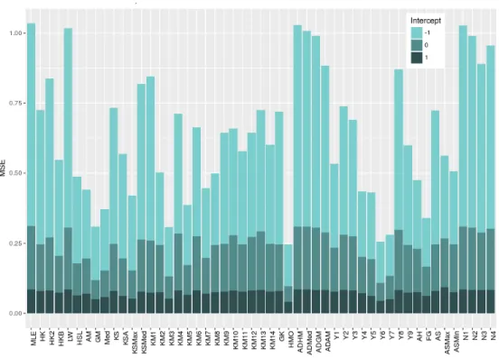
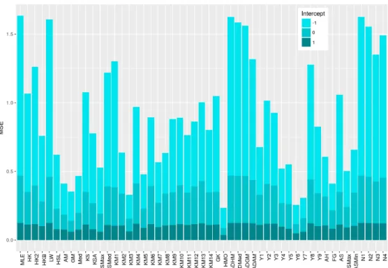
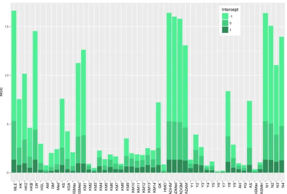
Figure 3.1 shows the MSE of each k estimator at each intercept, for

ρ

=

.

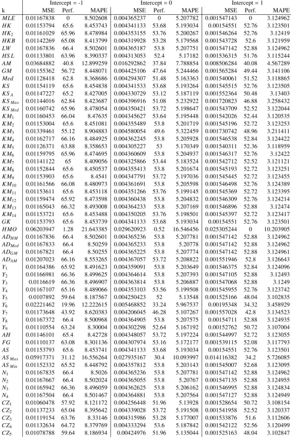
85. Tables for

other correlation values can be found in the Appendix. The tables 3.1 through 3.3 show

some of the simulation results. Full simulation results are available in the appendix.

(25)

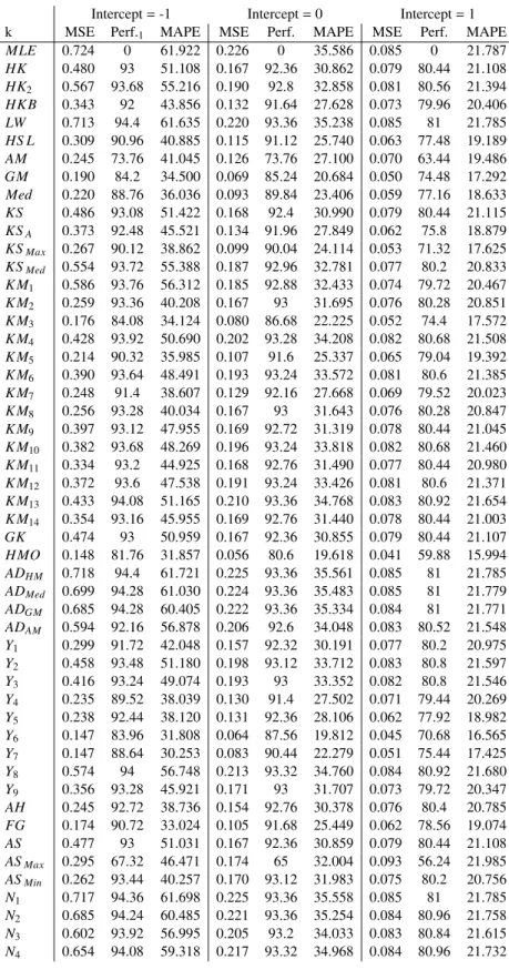
Table 3.1:

=

4, n

=

35, Correlation(

ρ

)

=

.

85

1. Performance

=

Percentage of times PRR outperforms MLE

Intercept=-1 Intercept=0 Intercept=1

k MSE Perf.1 MAPE MSE Perf. MAPE MSE Perf. MAPE

MLE 0.724 0 61.922 0.226 0 35.586 0.085 0 21.787 HK 0.480 93 51.108 0.167 92.36 30.862 0.079 80.44 21.108 HK2 0.567 93.68 55.216 0.190 92.8 32.858 0.081 80.56 21.394 HK B 0.343 92 43.856 0.132 91.64 27.628 0.073 79.96 20.406 LW 0.713 94.4 61.635 0.220 93.36 35.238 0.085 81 21.785 HS L 0.309 90.96 40.885 0.115 91.12 25.740 0.063 77.48 19.189 AM 0.245 73.76 41.045 0.126 73.76 27.100 0.070 63.44 19.486 GM 0.190 84.2 34.500 0.069 85.24 20.684 0.050 74.48 17.292 Med 0.220 88.76 36.036 0.093 89.84 23.406 0.059 77.16 18.633 KS 0.486 93.08 51.422 0.168 92.4 30.990 0.079 80.44 21.115 KSA 0.373 92.48 45.521 0.134 91.96 27.849 0.062 75.8 18.879 KSMax 0.267 90.12 38.862 0.099 90.04 24.114 0.053 71.32 17.625 KSMed 0.554 93.72 55.388 0.187 92.96 32.781 0.077 80.2 20.833 K M1 0.586 93.76 56.312 0.185 92.88 32.433 0.074 79.72 20.467 K M₂ 0.259 93.36 40.208 0.167 93 31.695 0.076 80.28 20.851 K M3 0.176 84.08 34.124 0.080 86.68 22.225 0.052 74.4 17.572 K M4 0.428 93.92 50.690 0.202 93.28 34.208 0.082 80.68 21.508 K M5 0.214 90.32 35.985 0.107 91.6 25.337 0.065 79.04 19.392 K M₆ 0.390 93.64 48.491 0.193 93.24 33.572 0.081 80.6 21.385 K M7 0.248 91.4 38.607 0.129 92.16 27.668 0.069 79.52 20.023 K M8 0.256 93.28 40.034 0.167 93 31.643 0.076 80.28 20.847 K M9 0.397 93.12 47.955 0.169 92.72 31.319 0.078 80.44 21.045 K M₁₀ 0.382 93.68 48.269 0.196 93.24 33.818 0.082 80.68 21.460 K M11 0.334 93.2 44.925 0.168 92.76 31.490 0.077 80.44 20.980 K M12 0.372 93.6 47.538 0.191 93.24 33.426 0.081 80.6 21.371 K M13 0.433 94.08 51.165 0.210 93.36 34.768 0.083 80.92 21.654 K M₁₄ 0.354 93.16 45.955 0.169 92.76 31.440 0.078 80.44 21.003 GK 0.474 93 50.959 0.167 92.36 30.855 0.079 80.44 21.107 H MO 0.148 81.76 31.857 0.056 80.6 19.618 0.041 59.88 15.994 ADH M 0.718 94.4 61.721 0.225 93.36 35.561 0.085 81 21.785 ADMed 0.699 94.28 61.030 0.224 93.36 35.483 0.085 81 21.779 ADGM 0.685 94.28 60.405 0.222 93.36 35.334 0.084 81 21.771 ADAM 0.594 92.16 56.878 0.206 92.6 34.048 0.083 80.52 21.548 Y1 0.299 91.72 42.048 0.157 92.32 30.191 0.077 80.2 20.975 Y₂ 0.458 93.48 51.180 0.198 93.12 33.712 0.083 80.8 21.597 Y3 0.416 93.24 49.074 0.193 93 33.352 0.082 80.8 21.546 Y4 0.235 89.52 38.039 0.130 91.4 27.502 0.071 79.44 20.269 Y5 0.238 92.44 38.120 0.131 92.36 28.106 0.062 77.92 18.982 Y₆ 0.147 83.96 31.808 0.064 87.56 19.812 0.045 70.68 16.565 Y7 0.147 88.64 30.253 0.083 90.44 22.279 0.051 75.44 17.425 Y8 0.574 94 56.748 0.213 93.32 34.760 0.084 80.92 21.680 Y₉ 0.356 93.28 45.921 0.171 93 31.707 0.073 79.72 20.347 AH 0.245 92.72 38.736 0.154 92.76 30.378 0.076 80.4 20.785 FG 0.174 90.72 33.024 0.105 91.68 25.449 0.062 78.56 19.074 AS 0.477 93 51.031 0.167 92.36 30.859 0.079 80.44 21.108 ASMax 0.295 67.32 46.471 0.174 65 32.004 0.093 56.24 21.985 ASMin 0.262 93.44 40.257 0.170 93.12 31.983 0.075 80.2 20.756 N1 0.717 94.36 61.698 0.225 93.36 35.558 0.085 81 21.785 N2 0.685 94.24 60.485 0.221 93.36 35.254 0.084 80.96 21.758 N₃ 0.602 93.92 56.995 0.205 93.2 34.033 0.083 80.84 21.615 N4 0.654 94.08 59.318 0.217 93.32 34.968 0.084 80.96 21.732

(26)

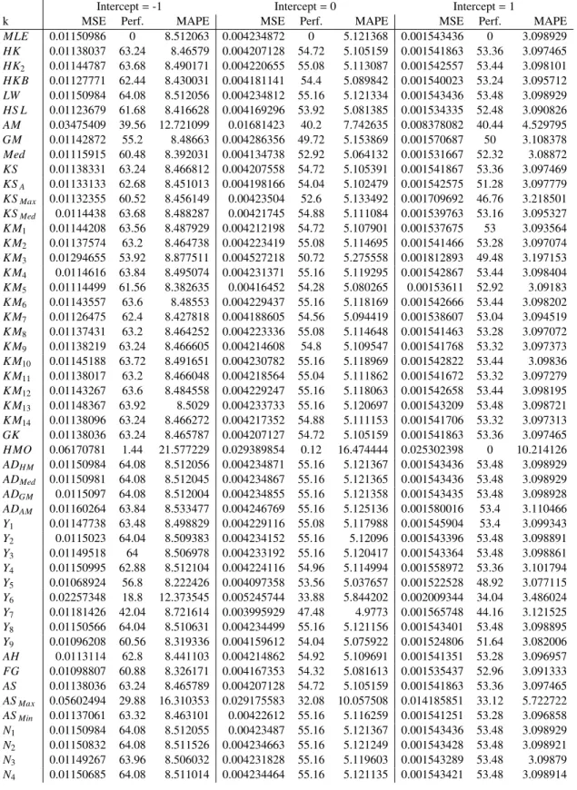
Table 3.2:

=

4, n

=

600,

ρ

=

.

85

k MSE Perf. MAPE MSE Perf. MAPE MSE Perf. MAPE

MLE 0.01150986 0 8.512063 0.004234872 0 5.121368 0.001543436 0 3.098929 HK 0.01138037 63.24 8.46579 0.004207128 54.72 5.105159 0.001541863 53.36 3.097465 HK2 0.01144787 63.68 8.490171 0.004220655 55.08 5.113087 0.001542557 53.44 3.098101 HK B 0.01127771 62.44 8.430031 0.004181141 54.4 5.089842 0.001540023 53.24 3.095712 LW 0.01150984 64.08 8.512056 0.004234812 55.16 5.121334 0.001543436 53.48 3.098929 HS L 0.01123679 61.68 8.416628 0.004169296 53.92 5.081385 0.001534335 52.48 3.090826 AM 0.03475409 39.56 12.721099 0.01681423 40.2 7.742635 0.008378082 40.44 4.529795 GM 0.01142872 55.2 8.48663 0.004286356 49.72 5.153869 0.001570687 50 3.108378 Med 0.01115915 60.48 8.392031 0.004134738 52.92 5.064132 0.001531667 52.32 3.08872 KS 0.01138331 63.24 8.466812 0.004207558 54.72 5.105391 0.001541867 53.36 3.097469 KSA 0.01133133 62.68 8.451013 0.004198166 54.04 5.102479 0.001542575 51.28 3.097779 KSMax 0.01132355 60.52 8.456149 0.00423504 52.6 5.133492 0.001709692 46.76 3.218501 KSMed 0.0114438 63.68 8.488287 0.00421745 54.88 5.111084 0.001539763 53.16 3.095327 K M1 0.01144208 63.56 8.487929 0.004212198 54.72 5.107901 0.001537675 53 3.093564 K M2 0.01137574 63.2 8.464738 0.004223419 55.08 5.114695 0.001541466 53.28 3.097074 K M3 0.01294655 53.92 8.877511 0.004527218 50.72 5.275558 0.001812893 49.48 3.197153 K M₄ 0.0114616 63.84 8.495074 0.004231371 55.16 5.119295 0.001542867 53.44 3.098404 K M5 0.01114499 61.56 8.382635 0.00416452 54.28 5.080265 0.00153611 52.92 3.09183 K M6 0.01143557 63.6 8.48553 0.004229437 55.16 5.118169 0.001542666 53.44 3.098202 K M₇ 0.01126475 62.4 8.427818 0.004188605 54.56 5.094419 0.001538607 53.04 3.094519 K M8 0.01137431 63.2 8.464252 0.004223336 55.08 5.114648 0.001541463 53.28 3.097072 K M9 0.01138219 63.24 8.466605 0.004214608 54.8 5.109547 0.001541768 53.32 3.097373 K M10 0.01145188 63.72 8.491651 0.004230782 55.16 5.118969 0.001542822 53.44 3.09836 K M₁₁ 0.01138017 63.2 8.466048 0.004218564 55.04 5.111862 0.001541672 53.32 3.097279 K M12 0.01143267 63.6 8.484558 0.004229247 55.16 5.118063 0.001542658 53.44 3.098195 K M13 0.01148367 63.92 8.5029 0.004233733 55.16 5.120697 0.001543209 53.48 3.098721 K M14 0.01138096 63.24 8.466272 0.004217352 54.88 5.111153 0.001541706 53.32 3.097313 GK 0.01138036 63.24 8.465787 0.004207127 54.72 5.105159 0.001541863 53.36 3.097465 H MO 0.06170781 1.44 21.577229 0.029389854 0.12 16.474444 0.025302398 0 10.214126 ADH M 0.01150984 64.08 8.512056 0.004234871 55.16 5.121367 0.001543436 53.48 3.098929 ADMed 0.01150981 64.08 8.512045 0.004234867 55.16 5.121365 0.001543436 53.48 3.098929 ADGM 0.0115097 64.08 8.512004 0.004234855 55.16 5.121358 0.001543435 53.48 3.098928 ADAM 0.01160264 63.84 8.533477 0.004246769 55.16 5.125136 0.001580016 53.4 3.110466 Y1 0.01147738 63.48 8.498829 0.004229116 55.08 5.117988 0.001545904 53.4 3.099343 Y2 0.0115023 64.04 8.509383 0.004234152 55.16 5.12096 0.001543396 53.48 3.098891 Y₃ 0.01149518 64 8.506978 0.004233192 55.16 5.120417 0.001543364 53.48 3.098861 Y4 0.01150995 62.88 8.512104 0.004224116 54.96 5.114994 0.001558972 53.36 3.101794 Y5 0.01068924 56.8 8.222426 0.004097358 53.56 5.037657 0.001522528 48.92 3.077115 Y6 0.02257348 18.8 12.373545 0.005245744 33.88 5.844202 0.002009344 34.04 3.486024 Y₇ 0.01181426 42.04 8.721614 0.003995929 47.48 4.9773 0.001565748 44.16 3.121525 Y8 0.01150566 64.04 8.510631 0.004234499 55.16 5.121156 0.001543401 53.48 3.098895 Y9 0.01096208 60.56 8.319336 0.004159612 54.04 5.075922 0.001524806 51.64 3.082006 AH 0.0113114 62.8 8.441103 0.004214862 54.92 5.109691 0.001541351 53.28 3.096957 FG 0.01098807 60.88 8.326171 0.004167353 54.32 5.081613 0.001535437 52.96 3.091333 AS 0.01138036 63.24 8.465789 0.004207128 54.72 5.105159 0.001541863 53.36 3.097465 ASMax 0.05602494 29.88 16.310353 0.029175583 32.08 10.057508 0.014185851 33.12 5.722722 ASMin 0.01137061 63.32 8.463101 0.00422612 55.16 5.116259 0.001541251 53.28 3.096858 N1 0.01150984 64.08 8.512055 0.00423487 55.16 5.121367 0.001543436 53.48 3.098929 N2 0.01150832 64.08 8.511526 0.004234663 55.16 5.121249 0.001543428 53.48 3.098921 N3 0.01149267 63.96 8.506032 0.004231828 55.16 5.119603 0.001543289 53.48 3.09879 N₄ 0.01150685 64.08 8.511014 0.004234464 55.16 5.121135 0.001543421 53.48 3.098914

(27)

Table 3.3:

MSE Ratios (10% Outliers), P

=

4, n

=

35

ρ

=

.

85

ρ

=

.

90

ρ

=

.

95

ρ

=

.

99

k

-1

0

1

-1

0

1

-1

0

1

-1

0

1

MLE

0.548

0.236

0.094

0.524

0.228

0.091

0.505

0.223

0.086

0.518

0.218

0.086

HK

0.469

0.192

0.089

0.427

0.176

0.084

0.384

0.155

0.074

0.338

0.122

0.053

HK

2

0.497

0.21

0.091

0.46

0.196

0.087

0.421

0.179

0.079

0.392

0.151

0.064

HK B

0.407

0.166

0.085

0.358

0.146

0.078

0.306

0.12

0.064

0.258

0.086

0.038

LW

0.547

0.232

0.094

0.521

0.221

0.091

0.5

0.209

0.086

0.49

0.179

0.086

HS L

0.424

0.17

0.079

0.359

0.142

0.069

0.316

0.113

0.047

0.258

0.075

0.022

AM

0.628

0.296

0.138

0.52

0.207

0.097

0.353

0.121

0.053

0.144

0.039

0.016

GM

0.38

0.13

0.071

0.303

0.098

0.056

0.219

0.061

0.037

0.194

0.044

0.017

Med

0.366

0.142

0.077

0.304

0.12

0.065

0.24

0.088

0.048

0.2

0.057

0.025

KS

0.471

0.193

0.089

0.43

0.177

0.084

0.386

0.156

0.074

0.339

0.122

0.053

KS

A

0.465

0.193

0.082

0.418

0.176

0.072

0.383

0.148

0.054

0.307

0.104

0.035

KS

Max

0.441

0.182

0.082

0.385

0.154

0.066

0.336

0.121

0.044

0.234

0.074

0.022

KS

Med

0.509

0.216

0.09

0.481

0.208

0.085

0.462

0.197

0.078

0.461

0.182

0.069

K M

1

0.522

0.216

0.087

0.495

0.207

0.083

0.476

0.198

0.074

0.479

0.184

0.066

K M

2

0.398

0.217

0.093

0.365

0.215

0.088

0.335

0.21

0.085

0.294

0.201

0.098

K M

3

0.449

0.167

0.082

0.375

0.139

0.068

0.277

0.097

0.048

0.136

0.044

0.022

K M

4

0.465

0.229

0.094

0.434

0.229

0.091

0.413

0.226

0.089

0.381

0.242

0.111

K M

5

0.356

0.157

0.081

0.298

0.139

0.072

0.238

0.106

0.056

0.152

0.057

0.028

K M

6

0.447

0.225

0.094

0.418

0.223

0.09

0.395

0.218

0.087

0.346

0.218

0.101

K M

7

0.37

0.173

0.085

0.316

0.157

0.076

0.258

0.126

0.062

0.169

0.069

0.035

K M

8

0.397

0.216

0.093

0.363

0.215

0.088

0.334

0.209

0.085

0.293

0.2

0.097

K M

9

0.436

0.198

0.09

0.389

0.184

0.085

0.337

0.159

0.074

0.236

0.101

0.049

K M

10

0.438

0.225

0.094

0.406

0.224

0.09

0.383

0.219

0.088

0.341

0.228

0.108

K M

11

0.412

0.203

0.09

0.367

0.193

0.085

0.317

0.169

0.076

0.212

0.109

0.054

K M

12

0.438

0.224

0.094

0.406

0.221

0.09

0.383

0.215

0.087

0.333

0.214

0.1

K M

13

0.462

0.234

0.095

0.44

0.237

0.092

0.441

0.246

0.094

0.494

0.356

0.164

K M

14

0.419

0.201

0.09

0.373

0.189

0.085

0.321

0.165

0.075

0.214

0.103

0.051

GK

0.467

0.192

0.089

0.424

0.176

0.084

0.381

0.155

0.074

0.322

0.121

0.053

H MO

0.583

0.293

0.158

0.475

0.191

0.105

0.295

0.091

0.05

0.17

0.042

0.016

AD

H M

0.546

0.235

0.094

0.522

0.227

0.091

0.501

0.223

0.086

0.512

0.217

0.086

AD

Med

0.541

0.235

0.094

0.513

0.226

0.091

0.493

0.221

0.086

0.501

0.215

0.085

AD

GM

0.534

0.233

0.094

0.505

0.225

0.091

0.488

0.219

0.086

0.497

0.213

0.085

AD

AM

0.495

0.221

0.093

0.466

0.215

0.089

0.446

0.208

0.083

0.449

0.196

0.081

Y

1

0.374

0.189

0.09

0.315

0.173

0.084

0.245

0.138

0.072

0.117

0.063

0.041

Y

2

0.44

0.214

0.093

0.382

0.201

0.089

0.316

0.177

0.081

0.184

0.106

0.06

Y

3

0.425

0.212

0.092

0.371

0.198

0.088

0.296

0.172

0.08

0.153

0.087

0.055

Y

4

0.365

0.174

0.087

0.308

0.155

0.078

0.229

0.116

0.064

0.106

0.048

0.031

Y

5

0.441

0.225

0.096

0.412

0.223

0.091

0.421

0.227

0.089

0.427

0.259

0.114

Y

6

0.722

0.283

0.133

0.718

0.279

0.135

0.748

0.276

0.143

0.993

0.365

0.218

Y

7

0.513

0.232

0.109

0.495

0.234

0.108

0.494

0.241

0.115

0.629

0.299

0.181

Y

8

0.495

0.226

0.093

0.453

0.216

0.09

0.411

0.201

0.083

0.328

0.163

0.073

Y

9

0.477

0.232

0.094

0.465

0.233

0.092

0.459

0.237

0.092

0.439

0.242

0.111

AH

0.399

0.206

0.093

0.365

0.204

0.088

0.331

0.194

0.085

0.292

0.182

0.1

FG

0.38

0.179

0.085

0.337

0.169

0.078

0.299

0.148

0.066

0.23

0.109

0.051

AS

0.468

0.192

0.089

0.426

0.176

0.084

0.382

0.155

0.074

0.329

0.122

0.053

AS

Max

0.82

0.495

0.224

0.757

0.356

0.155

0.562

0.226

0.08

0.414

0.07

0.022

AS

Min

0.429

0.233

0.097

0.414

0.238

0.093

0.415

0.255

0.097

0.471

0.335

0.162

N

1

0.546

0.235

0.094

0.521

0.227

0.091

0.501

0.223

0.086

0.512

0.217

0.086

N

2

0.535

0.232

0.094

0.508

0.223

0.091

0.483

0.216

0.086

0.482

0.206

0.084

N

3

0.507

0.22

0.093

0.47

0.208

0.089

0.431

0.193

0.082

0.397

0.166

0.072

N

4

0.525

0.229

0.094

0.495

0.219

0.09

0.467

0.211

0.085

0.456

0.198

0.082

(28)

3.3

β

0

Simulations were varied by intercept value. The intercept values included were

β

0

=

−

1

,

0

,

1. Performance, defined as the percentage of times that the estimator had a smaller

MSE than the maximum likelihood model, decreased with an increase in intercept value.

Both MAPE and MSE decreased with an increase in intercept value, which implies higher

accuracy. The intercept value of

β

0

=

1 produced the lowest MSE values.

3.4

Performance as a Function of

ρ

Simulations were varied by correlation. The coe

ffi

cient of correlation values used were

ρ

=

.

85

, .

90

, .

95

, .

99. Larger correlation values increased performance percentage, but also

increased MSE and MAPE values, with the largest values at

ρ

=

.

99.

3.5

n

Simulations were varied by sample size (

n

). Simulations were run using the sample size

n

=

35 and

n

=

600. Generally, the larger sample size produced much smaller MSE

values. It is also notable that the larger sample size a

ff

ected the performance of individual

k estimators. With

n

=

35, the k estimators with the lowest MSE values were

Y

6

,

Y

7

,

H MO

,

FG

,

K M

2

,

K M

3

,

AM

,

AH

,

K M

2

,

K M

8

,

AS

Min

, and

AS

Max

. With

n

=

600, the k

estimators with the lowest MSE values were

FG

,

Y

9

,

GM

,

HS L

,

Med

, and

Y

5

.

3.6

Best Performing Estimators

Estimators were judged by their MSE value at both sample sizes, and performance with

outliers. The k estimators that produced the lowest MSE values were selected.

Perfor-mance with outliers was considered secondarily. The k estimators which produced the

smallest MSE values are as follows:

FG

,

Y

5

,

Y

9

,

AH

,

K M

2

, and

K M

8

.

(29)

3.7

Proposed New Estimators

The following new estimators are proposed based on the seven best performing k

estima-tors:

1.

CZ

1

=

HarmonicMean

{

FG

,

Y

5

,

Y

9

,

AH

,

K M

2

,

K M

8

}

2.

CZ

2

=

GeometricMean

{

FG

,

Y

5

,

Y

9

,

AH

,

K M

2

,

K M

8

}

3.

CZ

3

=

ArithmeticMean

{

FG

,

Y

5

,

Y

9

,

AH

,

K M

2

,

K M

8

}

4.

CZ

4

=

Median

{

FG

,

Y

5

,

Y

9

,

AH

,

K M

2

,

K M

8

}

5.

CZ

5

=

Maximum

{

FG

,

Y

5

,

Y

9

,

AH

,

K M

2

,

K M

8

}

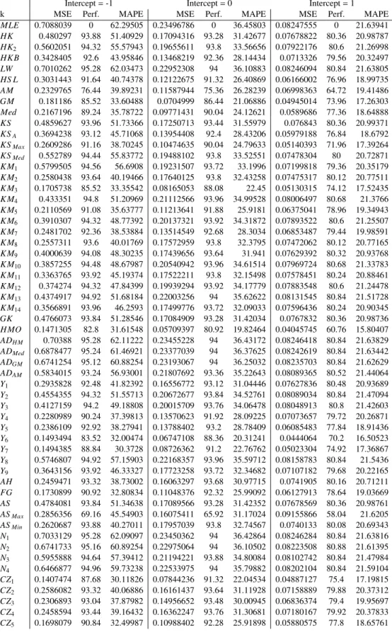
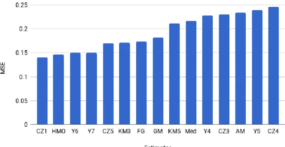
3.8

Performance of New Estimators

Simulations were then run again using these five new estimators. All five estimators

per-formed fairly well. The best performing estimators were

CZ

1

,

CZ

5

, and

CZ

3

.

CZ

1

fre-quently had a much smaller MSE than all other estimators. Figure 3.2 shows the MSE for

the 15 best performing estimators (n

=

35,

ρ

=

.

85,

β

0

=

−

1). See Tables 3.4 and 3.5 and

(30)

Table 3.4:

=

4, n

=

35,

ρ

=

.

85

MLE 0.7088039 0 62.29505 0.23496786 0 36.45803 0.08247555 0 21.63941 HK 0.480297 93.88 51.40929 0.17094316 93.28 31.42677 0.07678822 80.36 20.98787 HK2 0.5602051 94.32 55.57943 0.19655611 93.8 33.56656 0.07922176 80.6 21.26998 HK B 0.3428405 92.6 43.95846 0.13468219 92.36 28.14434 0.0713326 79.56 20.32497 LW 0.7010262 95.28 62.03473 0.22952308 94 36.10883 0.08246094 80.84 21.63805 HS L 0.3031443 91.64 40.74378 0.12122675 91.32 26.40869 0.06166002 76.96 18.99735 AM 0.2329765 76.44 39.89231 0.11587944 75.36 26.28239 0.06998363 64.72 19.41486 GM 0.181186 85.52 33.60488 0.0704999 86.44 21.06886 0.04945014 73.96 17.26303 Med 0.2167196 89.24 35.78722 0.09771431 90.04 24.12621 0.0589686 77.36 18.64888 KS 0.4859627 93.96 51.73366 0.17250713 93.44 31.55979 0.076843 80.36 20.99371 KSA 0.3694238 93.12 45.71068 0.13954408 92.4 28.43206 0.05979188 76.84 18.6792 KSMax 0.2609286 91.16 38.70245 0.10474635 90.04 24.79633 0.05140393 71.96 17.39264 KSMed 0.552789 94.44 55.83772 0.19488102 93.8 33.52551 0.07478304 80 20.72871 K M1 0.5799505 94.56 56.6908 0.19231507 93.72 33.1996 0.07199818 79.36 20.35179 K M2 0.2580438 93.64 40.19466 0.17640125 93.8 32.43258 0.07475317 80.12 20.77511 K M3 0.1705738 85.52 33.35542 0.08165053 88.08 22.45 0.05130315 74.12 17.52435 K M4 0.433351 94.8 51.20969 0.21112566 93.96 34.99528 0.08006497 80.68 21.3766 K M5 0.2110569 91.08 35.63777 0.11213641 91.88 25.9181 0.06375041 78.96 19.34943 K M6 0.3910307 94.32 48.77392 0.20137321 93.92 34.31872 0.07893522 80.6 21.25507 K M7 0.2481702 92.36 38.53884 0.13514549 92.68 28.3034 0.06853487 79.44 19.98591 K M8 0.2557311 93.6 40.01769 0.17572959 93.8 32.3795 0.07472062 80.12 20.77165 K M9 0.4000639 94.08 48.30235 0.17439656 93.64 31.941 0.07629392 80.32 20.93768 K M10 0.3857255 94.48 48.67987 0.20540942 93.96 34.61514 0.07969724 80.68 21.33783 K M11 0.3363765 93.92 45.19374 0.17522211 93.8 32.15498 0.07578451 80.24 20.88461 K M12 0.374274 94.32 47.84399 0.19939294 93.92 34.17779 0.07883548 80.6 21.24478 K M13 0.4374917 94.92 51.68184 0.22003256 94 35.62622 0.08131545 80.84 21.51728 K M14 0.3566891 93.96 46.2593 0.17499776 93.72 32.09033 0.07596436 80.24 20.90345 GK 0.4766073 93.84 51.28546 0.17084909 93.28 31.42034 0.0767832 80.36 20.98736 H MO 0.1471305 82.8 31.61548 0.05709397 80.92 19.82464 0.04045745 60.76 15.80407 ADH M 0.70388 95.28 62.11222 0.23455228 94 36.43172 0.08246418 80.84 21.63829 ADMed 0.6878477 95.24 61.46921 0.23377039 94 36.37625 0.08242619 80.84 21.63442 ADGM 0.6741254 95.12 60.88254 0.23193067 94 36.25032 0.08235703 80.84 21.62629 ADAM 0.5834015 93.24 56.93001 0.21807692 93.36 35.22643 0.08089365 80.52 21.44064 Y1 0.2935828 92.48 41.82392 0.16556772 93.12 31.04446 0.07627836 80.48 20.93689 Y2 0.4554355 94.32 51.55713 0.20672677 93.84 34.52761 0.08089034 80.84 21.47094 Y3 0.4127159 94.2 49.18808 0.20015709 93.76 34.06478 0.08048913 80.8 21.42603 Y4 0.2280989 90.24 37.39813 0.13570623 91.92 28.09225 0.07073657 79.72 20.26871 Y5 0.2386109 92.92 38.27941 0.13788402 93.2 28.78409 0.06085483 77.84 18.91436 Y6 0.1493494 83.52 32.00474 0.06747108 88.36 20.31241 0.0444064 70.2 16.50523 Y7 0.1494385 88.84 30.3728 0.08726362 91.2 22.76762 0.05023304 74.92 17.36867 Y8 0.5746807 94.92 57.15903 0.22168357 93.96 35.59712 0.08158783 80.84 21.5436 Y9 0.3643156 93.92 46.33327 0.17723258 93.72 32.34682 0.07107182 79.68 20.22165 AH 0.2459471 93.32 38.73002 0.16063297 93.68 30.97715 0.0741905 80.16 20.71211 FG 0.1730899 90.92 32.80834 0.11048376 92.32 25.99092 0.06127913 78.64 19.03669 AS 0.4784081 93.84 51.34638 0.17089566 93.28 31.42352 0.07678569 80.36 20.98761 ASMax 0.2856356 69.16 45.54903 0.16075411 65.92 31.17024 0.09155866 58.04 21.6205 ASMin 0.2620687 93.88 40.27011 0.17957039 93.8 32.74567 0.0740133 80.08 20.69343 N1 0.7033129 95.28 62.09097 0.23450362 94 36.42864 0.08246284 80.84 21.63816 N2 0.6741733 95.16 60.89254 0.22975064 94 36.10502 0.08223508 80.88 21.61395 N3 0.5955888 94.64 57.39412 0.21194221 93.88 34.80084 0.08102742 80.84 21.47984 N4 0.6466877 94.96 59.73238 0.22533975 94 35.79882 0.08202104 80.84 21.59104 CZ1 0.1407474 87.68 30.11826 0.07844236 91.32 22.04534 0.04887127 75.4 17.19815 CZ2 0.2586082 93.32 40.06886 0.16161437 93.64 31.11928 0.07158889 79.88 20.37312 CZ3 0.2306893 93.04 37.87982 0.14956652 93.48 30.00945 0.06836374 79.4 19.95697 CZ4 0.2458594 93.44 39.16432 0.16362247 93.76 31.30681 0.07180167 79.92 20.37833 CZ5 0.1698079 90.84 32.49987 0.10988402 92.28 25.91898 0.05880575 77.8 18.65761

(31)

Table 3.5: Poisson Regression Simulation Results (New Estimators), P

=

4, n

=

600,

ρ

=

.

85

MLE 0.01167838 0 8.502608 0.004365237 0 5.207782 0.001547143 0 3.124962 HK 0.01153794 65.6 8.453743 0.004341133 53.68 5.193034 0.00154551 52.76 3.123501 HK2 0.01161029 65.96 8.478984 0.004353155 53.76 5.200267 0.001546264 52.76 3.12419 HK B 0.01142269 65.08 8.413799 0.004319928 53.28 5.179568 0.001543728 52.6 3.121959 LW 0.01167836 66.4 8.502601 0.004365187 53.8 5.207751 0.001547142 52.88 3.124962 HS L 0.01133801 63.96 8.390337 0.004313053 52.4 5.17182 0.001536315 51.76 3.115244 AM 0.03684882 40.8 12.899259 0.016292862 37.84 7.788854 0.008506284 40.08 4.567289 GM 0.01155362 56.72 8.448071 0.004425106 47.64 5.244466 0.001565284 49.44 3.141106 Med 0.01128418 62.8 8.368686 0.004294307 51.48 5.163363 0.001540061 51.52 3.118865 KS 0.01154119 65.6 8.454838 0.004341533 53.68 5.193264 0.001545515 52.76 3.123505 KSA 0.01147227 65.2 8.427005 0.004330729 53.12 5.187119 0.001552364 50.48 3.13403 KSMax 0.01144016 62.84 8.423687 0.004396916 51.08 5.232922 0.001720823 46.88 3.258432 KSMed 0.01160742 65.96 8.478054 0.004350421 53.72 5.198647 0.001543709 52.52 3.122044 K M1 0.01160453 66.04 8.47635 0.004345627 53.64 5.195448 0.001542026 52.44 3.120535 K M2 0.01153004 65.6 8.451081 0.004355489 53.8 5.201719 0.001545196 52.72 3.123253 K M3 0.01339461 55.12 8.904883 0.004580054 49.6 5.322459 0.001730742 48.96 3.211411 K M4 0.01162717 66.16 8.484925 0.004362245 53.8 5.205928 0.001546538 52.84 3.124422 K M5 0.01126371 63.88 8.358653 0.004305227 53 5.170349 0.001540311 52.36 3.118959 K M6 0.01159795 65.96 8.474695 0.004360609 53.8 5.204937 0.001546317 52.76 3.12422 K M7 0.01141122 65 8.409056 0.004325866 53.44 5.183524 0.001542712 52.52 3.121121 K M8 0.01152844 65.6 8.450537 0.004355413 53.8 5.201674 0.001545193 52.72 3.123251 K M9 0.01153903 65.6 8.4541 0.004347791 53.72 5.197036 0.001545445 52.72 3.123455 K M10 0.01161566 66.08 8.480973 0.004361691 53.8 5.205598 0.001546498 52.76 3.124389 K M11 0.01153611 65.6 8.453118 0.004351266 53.76 5.199145 0.001545369 52.72 3.123395 K M12 0.01159474 65.92 8.473598 0.004360438 53.8 5.204832 0.001546309 52.76 3.124214 K M13 0.01165043 66.32 8.493008 0.004364233 53.8 5.207169 0.001546896 52.88 3.12474 K M14 0.01153721 65.6 8.453488 0.004350205 53.76 5.198501 0.001545397 52.72 3.123417 GK 0.01153793 65.6 8.453739 0.004341133 53.68 5.193034 0.00154551 52.76 3.123501 H MO 0.06203947 1.28 21.643385 0.029620923 0.52 16.546456 0.025305244 0 10.203905 ADH M 0.01167836 66.4 8.502601 0.004365236 53.8 5.207781 0.001547142 52.88 3.124962 ADMed 0.01167833 66.4 8.50259 0.004365233 53.8 5.20778 0.001547142 52.88 3.124962 ADGM 0.01167821 66.4 8.50255 0.004365225 53.8 5.207774 0.001547142 52.88 3.124961 ADAM 0.01207023 66.16 8.553265 0.004367057 53.72 5.208822 0.001551946 52.8 3.126643 Y1 0.01164386 65.92 8.491623 0.004359091 53.8 5.203649 0.001546375 52.84 3.124096 Y2 0.01166981 66.36 8.499625 0.004364614 53.8 5.207393 0.001547105 52.88 3.12493 Y3 0.0116619 66.36 8.496907 0.004363814 53.8 5.206887 0.001547068 52.88 3.1249 Y4 0.01167107 65.16 8.489066 0.004353103 53.56 5.199508 0.001545955 52.76 3.123742 Y5 0.0107892 59.64 8.187567 0.004250423 52 5.13548 0.001525166 48.04 3.102835 Y6 0.02221462 19.96 12.222615 0.005468852 33.24 5.967537 0.00195348 34.32 3.458929 Y7 0.01173648 43.92 8.620383 0.004206045 46.28 5.107267 0.001557028 42.8 3.134523 Y8 0.01167372 66.4 8.500968 0.004364905 53.8 5.207575 0.00154711 52.88 3.124935 Y9 0.01110554 63.24 8.30004 0.004302298 52.64 5.167192 0.00152762 50.72 3.107004 AH 0.01146101 65.4 8.42728 0.004348057 53.72 5.197224 0.001544997 52.72 3.123055 FG 0.01110137 63.08 8.301136 0.004307974 53.16 5.172177 0.001539115 52.08 3.117793 AS 0.01153793 65.6 8.453741 0.004341133 53.68 5.193034 0.00154551 52.76 3.123501 ASMax 0.05917371 31.12 16.556264 0.027935167 30.4 10.093997 0.014116382 34.2 5.726085 ASMin 0.01152332 65.52 8.448792 0.004357812 53.8 5.203143 0.001545007 52.68 3.123095 N1 0.01167835 66.4 8.5026 0.004365236 53.8 5.207781 0.001547142 52.88 3.124962 N2 0.01167667 66.4 8.502024 0.004365055 53.8 5.20767 0.001547135 52.88 3.124955 N3 0.01165942 66.36 8.496059 0.004362625 53.8 5.206162 0.001546995 52.88 3.124834 N4 0.01167504 66.4 8.501467 0.004364881 53.8 5.207564 0.001547127 52.88 3.124949 CZ1 0.01060478 57.92 8.121172 0.004256448 51.96 5.13928 0.001528654 50.72 3.108154 CZ2 0.01137233 65.04 8.395642 0.004339028 53.72 5.191508 0.001541958 52.52 3.120337 CZ3 0.01119154 63.76 8.33146 0.004315986 53.28 5.177007 0.001533876 51.6 3.112606 CZ4 0.01132634 64.72 8.379769 0.004333294 53.6 5.187842 0.001542122 52.56 3.120499 CZ5 0.01078788 59.64 8.186934 0.00424976 51.96 5.135044 0.001525163 48.04 3.102847

(32)

(33)

CHAPTER 4

APPLICATION

The ridge estimators are applied here using data from a study of 659 individuals by Sellar

et al. (1985), which estimated the value of recreational boating in East Texas. Four lakes

were studied: Lakes Conroe, Livingston, Somerville, and Houston. The study tracked

the number of visits an individual has made to the lakes (NTrip), as well as their income

level, quality rating scores for the lakes, whether the individual has engaged in

water-skiing at Lake Somerville (SKI), whether the individual has paid an annual fee at Lake

Somerville (FEE), and the travel costs to Lakes Conroe, Somerville, and Houston (LC,

LS, and LH). The three cost variables (LC, LS, and LH) are highly correlated. The level

of multicollinearity is measured here using the Variance Inflation Factor (VIF). VIF is the

ratio of variance in the full model, with all terms, divided by the variance of a reduced

model, with only one term. With high VIF values (VIF greater than 3), the variance of

the estimated coe

ffi

cient is increased. Table 4.1 shows the VIF for each regressor. It is

clear from this table that LC, LS, and LH are highly correlated. In the case of severe

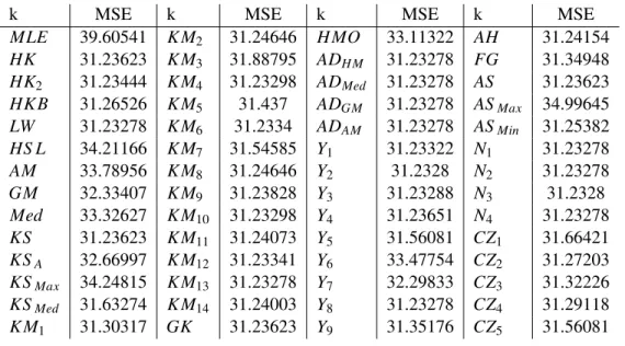
mul-ticollinearity, a ridge regression model is recommended. Table 4.2 shows the MSE values

of the MLE model and the 55 ridge regression models. All ridge estimators had a lower

MSE than the MLE model. The MLE model had an MSE of 39.61, while all of the ridge

models produced an MSE smaller than 35. Most k estimators performed fairly well, with

an MSE of about 31, including the five newly introduced estimators. Table 4.3 shows the

significance of the regression coe

ffi

cients of MLE and two of the best performing new

estimators,

CZ

1

and

CZ

3

. Table 4.4 shows the estimated regression coe

ffi

cients for each

model. All coe

ffi

cients had a positive slope, with the exception of LS, which consistently

had a negative coe

ffi

cient value. This means that the number of trips (NTrip) decreases as

(34)

LS, the travel cost to Lake Somerville, increases. The number of trips increases with an

increase in the other variables (FEE, LC, and LH).

Table 4.1: VIF for each regressor

SKI

FEE

LC

LS

LH

1.088497

1.024602

11.838841

3.188796

10.908486

Table 4.2:

MSE for Each k Estimator - Recreation Data

k

MSE

k

MSE

k

MSE

k

MSE

MLE

39.60541

K M

2

31.24646

H MO

33.11322

AH

31.24154

HK

31.23623

K M

₃

31.88795

AD

H M

31.23278

FG

31.34948