Beat-to-beat Variability of Repolarization Duration Measures for Automated Arrhythmia Prediction and their Relation to Cell Models

(1)

Automated Arrhythmia Prediction and their Relation to Cell Models

J. Heijman

June 15, 2006

Abstract

This article presents an overview of differ-ent measures for beat-to-beat variability of cardiac ventricular repolarization (BVR). Action potential duration (APD), variability of repolarization duration, Poincaré plot area, instability of repolarization and a combined measure are compared on their capabilities for the prediction of susceptibility to arrhythmias. This is done by both statistical comparison and k-fold crossvalidation on a set of action potential recordings from canine ventricular myocytes. The results: a low performance for APD and a better performance for measures based on Poincaré plots (short term variability, Poincaré plot area and combined variability), agree with findings by others. The Hund-Rudy dynamical cell model is analyzed for its BVR characteristics. However, it appears that there is too little coupling/connection between the variables in the model to realize this behaviour.

Keywords: action potentials, BVR, cell model

1

Introduction

Although cardiac electrophysiology has greatly advanced since the first graphic documentation of ventricular fib-rillation in 1884 [5], sudden cardiac death, mainly caused by ventricular fibrillation, still causes 450,000 deaths an-nually in the United States, making it the number one single cause of death [1, 18]. A first step in decreasing this number could be the identification and prediction of events in physiological signals that indicate upcom-ing ventricular tachy arrhythmias. These arrhythmias can degenerate into ventricular fibrillation, a condition that requires medical treatment by electrical cardiover-sion within a few minutes or else can result in sudden cardiac death [2]. A sufficiently early detection would therefore facilitate the medical treatment by giving the patient and medical staff a larger time-frame to respond.

A subset of these arrhythmic conditions occurs in the setting of repolarization prolongation. Prolongation of the QT interval in electrocardiograms and prolongation of action potential duration (APD) in single cell record-ings have long been associated with proarrhythmic ac-tivity [4]. However, in recent years it has become clear that fibrillation is a highly dynamical process, often with chaotic characteristics [17]. Combined with the observa-tion that QT interval and APD prolongaobserva-tion by them-selves are not necessarily proarrhytmic [7], this resulted in a new concept for identification and prediction incor-porating these dynamics: beat-to-beat variability of re-polarization duration (BVR). Thomsen et al. examined, among other things, the variability of the monophasic action potential duration of canine left ventricular en-docardium using Poincar´e plots [12]. They showed that this measure provided a better indication of susceptibil-ity for arrhythmia than QT interval prolongation.

The purpose of this research is the automation of the prediction of susceptibility for ventricular tachy arrhyth-mias using BVR measures as well as a further analysis on their predictive power from both a mathematical per-spective and their physiological application.

This paper is structured as follows: first an introduc-tion into the physiological background of acintroduc-tion poten-tials and ventricular repolarization is given. Then the automation of the prediction and the methods used to test this process are discussed. Afterwards, the test re-sults are given and the rere-sults are compared with the output of the Hund-Rudy dynamic cell model. Finally, the conclusions and recommendations are presented.

2

Physiological Background

2.1

Action Potential

The signals that are used in this research are transmem-brane action potential recordings of enzymatically iso-lated canine ventricular cells. These action potentials (APs) depict the membrane potential of a single cell versus time. At any point in time, this potential is the net result of ionic currents that are heterogeneously dis-tributed on the cellmembrane [6] and changes dynami-cally due to ion channel activity. These ion flows are,

(2)

in particular, sodium (N a+_{), potassium (}_K+_{), calcium}

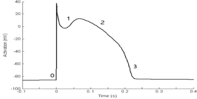
(Ca2+), chloride (Cl−) and hydrogen (H+). When an excitable cell receives a (electric) stimulus, it rapidly de-polarizes. Then, during approximately 200 ms, different ion channels open and close which results in a distinct action potential configuration [4] (Figure 1). An AP

con-Figure 1: Typical canine action potential sists of five phases. Phase 0 is the rapid depolarization as a result of the stimulus. Phase 1 is the early rapid repolarization phase, which can be followed by a notch. Phase 2 is the plateau phase and phase 3 is the final rapid repolarization phase. In the final phase, the mem-brane potential is again at resting level. However, the exact morphology of an AP can be different for cells from different regions of the heart.

The purpose of the AP is to co-ordinate the contrac-tion of the cell and, on a higher level, the contraccontrac-tion of the heart [13].

2.2

Action Potentials versus ECG

Another common recording in cardiology is the electro-cardiogram (ECG). The relation between APs and ECG signals is that they both represent electrical currents which are, more specifically, depolarization and repolar-ization currents in the heart. However, APs consist of the currents of a single cell or a few coupled cells. ECG signals on the other hand capture information from dif-ferent APs in various regions of the heart [13]. As a re-sult of this ionic currents, APs and ECG signals can be placed in an ordering of increasing complexity. In this research APs are used instead of ECG signals because the reduced complexity makes it possible to relate char-acteristics of the results to the major ionic charge car-riers. In particular, this can be done by comparing the results obtained from tests on recordings of real canine ventricular cells to those from a mathematical model.

2.3

BVR

As mentioned in the introduction, it has become appar-ent that repolarization interval prolongation is not a sen-sitive measure for arrhythmia prediction. Instead, it ap-peared that a strong variance in successive beats or APs

was a better measure to capture the dynamical nature of arrhythmias [7]. Beat-to-beat variability of repolar-ization (BVR) is, as its name suggests, a quantification of the variance between successive APs. In the single cell environments used in this research, there is only this temporal variability between successive APs. However, it must be emphasized that in multicellular environments and particularly in the heart, there is also spatial vari-ability between the repolarizations of different regions.

A series of APs, such as those illustrated in figure 2, can be described as a set of (time, value) pairs: SAP = {(t1, v1),(t2, v2), . . . ,(tn, vn)}. BVR is then defined as a

Figure 2: AP series

function:

BV R:SAP→_Rm ₍₁₎

whereBV R(SAP_{) increases as the variance between} con-secutive beats inSAP increases.

Thomsen et al. describe two different measures for BVR: Variability and Poincar´e plot area [12]. These measures, together with two other measures, are de-scribed below.

Variability

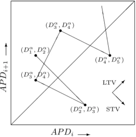
Short Term Variability (STV) is a BVR measure that uses Poincar´e plots to visualize the beat-to-beat vari-ability. In these Poincar´e plots the duration of an AP (APD) is plotted against the duration of the previous AP, as shown in Figure 3. This approach illustrates both the variability between consecutive beats as well as summary information. Moreover, these plots also cap-ture the non-linearity of the underlying processes [3]. In order to define STV, a function to extract AP durations has to be defined. Let

Tα(SAP) ={(s1, eα1),(s2, eα2), . . . ,(sp, eαp)} (2) be a function returning a set of start (s) and end (e) times for the APs in a seriesSAP_{. The parameter} _α_in equation 2 indicates the percentage of the baseline level that is considered to define the end of the AP, as shown in Figure 4. The AP durations are then given by:

(3)

r r r r r @ @ @ @ @ @ H H H H H H HH H H H HE E E E E E (Dα 1, D α 2) (Dα 2, D α 3) (Dα 3, D4α) (D₃α, Dα₄) (Dα 4, D α 5) @ @ R LTV STV 6 AP D i +1 AP Di

-Figure 3: Poincar´e plot with as inset arrows indicating the directions in which STV and LTV operate

Figure 4: Different repolarization levels

Dα(Tα(SAP)) ={eα1 −s1, eα2 −s2, . . . , eαp−sp}. (3) These durations can be displayed in a Poincar´e plot. Short term variability is defined as the average distance from the points in the plot to the line of identity (see Figure 3). This distance is given by:

ST V(Dα) = 1 p√2 p−1 X i=1 |D_iα₊₁−Dα_i |. (4)

Similarly long term variability (LTV) is defined as the average distance from the points to the mean of the pa-rameter orthogonal to the line of identity, or:

LT V(Dα) = 1 p√2 p−1 X i=1 |D_iα₊₁+D_iα−2D_meanα |. (5)

In this article, ST V(SAP_{) and} _{LT V}₍_SAP_{) are used} as a short hand notation for ST V(Dα₍_Tα₍_SAP_{))) and}

LT V(Dα₍_Tα₍_SAP_{))) for a given repolarization level}_α_.

Poincar´e plot area

The second BVR measure that uses AP durations in a Poincar´e plot is Poincar´e plot area (PCPA). Thomsen

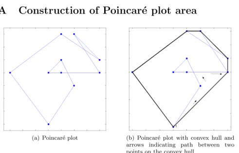
et al. argue that AP series exhibiting arrhythmogenic behaviour result in a Poincaré plot that has a larger area than plots from non-arrhythmogenic AP series [12]. The area of a Poincaré plot defined by points (D_iα, Dα_i₊₁) is calculated by following the outer-most lines between two adjacent points on the convex hull of the points. The area of the polygon bounded by these lines and the line connecting the two points on the convex hull is sub-tracted from the total area of the convex hull. If this pro-cedure is repeated for all points on the convex hull, the resulting area is the area of the polygon bounded by the outermost lines of the Poincaré plot, which is referred to as P CP A(SAP_{). This process is shown in Figure 12(a)} - 12(c) (appendix A). The advantage of PCPA with re-spect to STV and LTV is that it captures the total beat-to-beat variability. Further research has to be done in order to determine how STV and LTV can be combined in such a way that this single measure can adequately reflect arrhythmogenic behaviour. However, the main disadvantage of the Poincaré plot area is that there are infinitely many different Poincaré plots, with entirely dif-ferent arrhythmogenic outcomes that still have the same area.

Instability

An alternative BVR measure comparable to STV / LTV is described by Van der Linde et al. [14]. Their beat-to-beat instability has three components: short-term stability (STI), long-term instability (LTI) and total in-stability (TI). STI is, similar to STV, defined as the or-thogonal distance of AP durations in a Poincar´e plot to a 45◦ line. However, in STI this is not the line of iden-tity but the line y = x+b (parallel to the diagonal) that intersects the ’centre of gravity’ of the points. Let

rcgx and rcgy be the x and y co-ordinates of the cen-tre of gravity; rotated by−45◦ _{around the origin (using} cos(−1 4π) = 1 2 √ 2 and sin(−1 4π) =− 1 2 √ 2): cgx= 1 p p−1 X i=1 Dα_i (6) cgy= 1 p p X i=2 Dα_i (7) rcgx= 1 2 √ 2cgx+ 1 2 √ 2cgy (8) rcgy=− 1 2 √ 2cgx+ 1 2 √ 2cgy. (9) Then, STI is given by1:

ST I(Dα) =M|rcgy+ −√2Dα i+1+ √ 2Dα i 2 | . (10) 1_{Note that in the original paper [14] the first plus sign was}

(4)

Similarly, LTI is given by: LT I(Dα) =M|rcgx−( √ 2Dα_i₊₁ 2 + √ 2Dα_i 2 )| . (11) TI is defined as the median distance from the points to the center of gravity:

T I(Dα) =M q(cg(x)−Dα i)2+ (cg(y)−D α i+1)2 . (12) In equations 10, 11 and 12, Van der Linde et al. use median values (M) instead of mean values in order to reduce the effect of extreme values. Note that this is in contrast to the calculation of the variability measures and Poincar´e plot area, which are more sensitive to these values.

In this article, ST I(SAP_), _{LT I}₍_SAP_{) and} _{T I}₍_SAP₎ are used similar toST V(SAP).

Total combined variability

Total combined variability (TCV) is an attempt to com-bine the measures described by Thomsen et al. [12] in a single BVR measure. By combining STV, LTV and PCPA in a good way, differences between arrhythmo-genic and non-arrhythmoarrhythmo-genic signals can be enhanced, therefore allowing a better classification of new AP se-ries. TCV is defined as follows:

T CV(SAP) = (P CP A(SAP) +ST V(SAP)) ×

q

ST V(SAP₎2₊_{LT V}₍_SAP₎2_. ₍₁₃₎

The second part of equation 13 is chosen based on the definition of TI (equation 12) and the total equation has some desirable properties. First of all, TCV is an in-creasing function of all three components. Second, if an AP series exhibits only long term variability such as a steadily increasing APD, the TCV measure is equal to zero. This agrees with the results of Thomsen et al. that show that such behaviour is not necessarily arrhythmo-genic. Finally, if an AP series has only short term vari-ability then TCV reduces to a simple function of STV since the Poincar´e plot will be a line, which has an area of zero:

T CV(SAP) =ST V(SAP)2. (14) This behaviour is called beat-to-beat alternans since it results in APs that have alternating long and short du-rations.

The disadvantage of this BVR measure is that it is an empirically based combination of measures. As a result of this ’black-box’ approach, it is more difficult to relate the values and the performance of this measure to the physiological basis of an AP series. Moreover, it can not be guaranteed that this particular combination of BVR measures is the optimal combination. However, a measure such as TCV can be used to assess the utility of a second order (combined) BVR measure.

3

Test method

The quality of the different BVR measures discussed in section 2.3 is compared by applying the measures to a set of real canine ventricular AP series. This set is defined as follows:

S={(S1AP, λ1),(S2AP, λ2), . . . ,(SkAP, λk)}. (15) The label λi indicates whether or not the correspond-ing AP series SAP

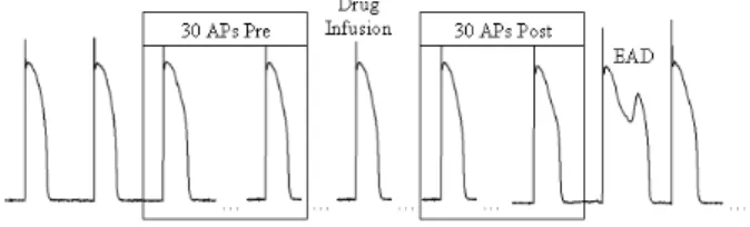
i exhibits arrhythmogenic behaviour. For this test set, all AP series consist of 2 times 30 APs from normal canine ventricular myocytes and are taken at a pacing length of 1000 ms. For a single cell, the first 30 APs are taken before the addition of a drug that is associated with proarrhythmic behaviour and these are hereby defined as non-arrhytmogenic (λi = 0). The se-ries that exhibit arrhythmogenic behaviour (λi= 1) are defined as the 30 beats after the addition of a class III drug, such as d-Sotalol, that is known for its proarrhyth-mic effects. If possible these APs were taken before the occurance of an early afterdepolarization (EAD). EADs are secondary depolarizations that occur before the end of the AP and are associated with arrhythmias in the complete heart [16]. Note that the two classes defined here reflect only cellular arrhythmogenisis. Figure 5 il-lustrates the selection process. A full overview of the test

Figure 5: Overview of the selection of two AP series from a cell

set and the respective BVR values is given in appendix B.

The quality of the BVR measures is compared by both statistical analysis and k-fold crossvalidation. These performance measures are described in the next two sections.

3.1

Statistical Comparison

Using the values from Tables 6 and 7 and assuming that these values arise from a normal distribution, the quality of a BVR measure can be determined by the area of the overlapping parts of the normal distribu-tions for the arrhythmogenic and non-arrhythmogenic signals. If the two distributions are completely separate, that is, have an overlapping area of approximately zero, they allow perfect classification of an AP series. If, on

(5)

the other hand, the two distributions completely coin-cide, no distinction between arrhythmogenic and non-arrhythmogenic behaviour can be made. This results in the following performance measure for a BVR measure

B. Let µN_B = 1 k1 k1 X i=1 B(S_iAP) (16) and σN_B = v u u t 1 k1−1 k1 X i=1 (B(SAP i )−µ N B)2 (17) be estimators for the mean and standard deviation of the BVR values for the non-arrhythmogenic AP se-ries. In equations 16 and 17 k1 is the number of

non-arrhythmogenic AP series in S (equation 15). Also, let

µA B andσ

A

B be defined similarly for the arrhythmogenic series. Then, the area of the overlapping region of the two normal distributions n(x;µN

B, σBN) andn(x;µAB, σBA) is given by: AB= Z ∞ −∞ min n(x;µN_B, σN_B), n(x;µA_B, σ_BA) dx (18) with n(x;µ, σ) = 1 σ√2πexp −(x−µ) 2 2σ2 . (19)

The performance of the BVR measure B is then:

PB = 1−AB (20)

which results in a value between zero (worst possible performance) and one (optimal performance).

3.2

K-fold crossvalidation

Since the number of samples is limited, it is difficult to assess if the normality assumption can be justified. Therefore, a second test is performed on the data from tables 6 and 7. In this k-fold crossvalidation test the entire setS (equation 15) is divided in a test setST est

and a training setST rain_{. The test set consists of} 100

k % of the items in the total set and the i-th part of the test set is chosen for fold i. For example, ifk= 4, in the first fold the first quarter is test set, in the second fold the second quarter, etc. The goal is then to classify the AP series in the test set as either exhibiting arrhythmogenic behaviour or not, based on information in the training set. This is done by comparing the BVR values of the current test AP series to the BVR values of the AP series in the training set. The classifications can be compared to the real labels λ to determine the performance of a BVR measure.

The functions used to classify an AP series based on information in the training set are described below.

Nearest neighbour classifier

The nearest neighbour classifier is based on the as-sumption that objects with the same characteristics (in this case: exhibiting arrhythmogenic behaviour or not) have similar representations (in this case: BVR values). Therefore, in order to classify an AP series, this classifier determines the distance between the test series and all series in the training set. The resulting classification is the label of the AP series that has the smallest distance to the test series. There are many variations on this clas-sifier: analyzing multiple neighbours, different distance metrics, etc. Here the most basic version is used: the 1-nearest neigbour with Euclidian distance. This classifier can be described by the following function:

C(S_testAP|ST rain) =λj (21) where j is the index of the AP series that has the smallest distance to the test series:

j= argmin_idB(SAP_test), B(S_iT rain), (22) d is the Euclidian distance metric

d(a, b) = v u u t m X j=1 (aj−bj)2 (23)

and B is a BVR measure. Note that, for the one-dimensional BVR measures discussed in section 2.3, equation 22 simplifies to:

j= argmini |B(StestAP)−B(SiT rain)|. (24) However, equation 1 does not restrict BVR values to be one-dimensional.

Statistical classifier

The statistical classifier is a classifier implementation of the statistical comparison process described in section 3.1. In order to classify a test AP series, the training set is first divided in two subsets: the AP series that exhibit arrhythmogenic behaviour and those that do not (as defined in the beginning of this chapter). Then the estimatorsµA_B, σ_BA, µN_B andσ_BN are calculated. Next, the probabilities that the test AP series arises from the two normal distributions are calculated

pA= Z ex+ e x− n(x;µA_B, σA_B)dx (25) pN = Z ex+ e x− n(x;µN_B, σ_BN)dx (26) where e x=B(S_testAP) (27)

(6)

andis a sufficiently small number. IfpA> pN, the test AP series is classified as arrhythmogenic. Otherwise it is classified as non arrhythmogenic. If the BVR measure B has more than one dimension, the probabilities for each dimension are averaged and the average values are compared.

4

Test results

4.1

Statistical comparison

Table 1 gives an overview of the estimators and the per-formance for the statistical comparison with a 90% re-polarization level (α= 0.9). This table shows that APD

µA B±σ A B µ N B±σ N B Performance APD 400±40.5 369±51.1 0.281 STV 20.9±05.2 09.9±04.3 0.758 LTV 31.1±14.9 11.9±05.3 0.718 PCPA 08.9±04.9 02.2±01.6 0.749 STI 13.3±06.1 07.3±03.2 0.527 LTI 21.0±05.8 18.0±03.1 0.369 TI 31.4±07.8 21.1±04.1 0.656 TCV 01.2±0.53 0.22±0.18 0.857

Table 1: Estimators and test results for statistical com-parison

is not a sensitive measure to detect arrhythmogenic be-haviour. It also shows that, from the three measures discussed by Thomsen et al. PCPA and STV have a similar performance and that this performance is signif-icantly better than that of APD. This agrees with their findings [12]. Moreover, it also illustrates that there is a significant difference between STV / LTV and STI / LTI although they are defined similarly (see section 2.3). The lower performance of the instability measures could be explained by the fact that the absolute location of the points in the Poincar´e plot is not taken into account. That is, if two Poincar´e plots have a similar form but occur at different locations (for example one on the line of identity and one far away), the instability measures still have very similar values. Besides, it is possible that the fact that instability uses median values instead of mean values, results in a situation where extreme APs (that might actually be the most important ones to in-vestigate) are not weighed as heavily as in STV or LTV. The final observation is that the new measure TCV, de-fined in section 2.3, has the best performance in this comparison. This is likely due to the fact that it com-bines three positively correlated measures. This results in a larger difference between the values of arrhythmo-genic and non-arrhythmoarrhythmo-genic series, which results in a higher performance.

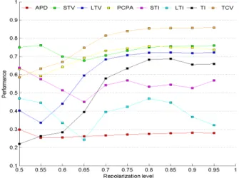
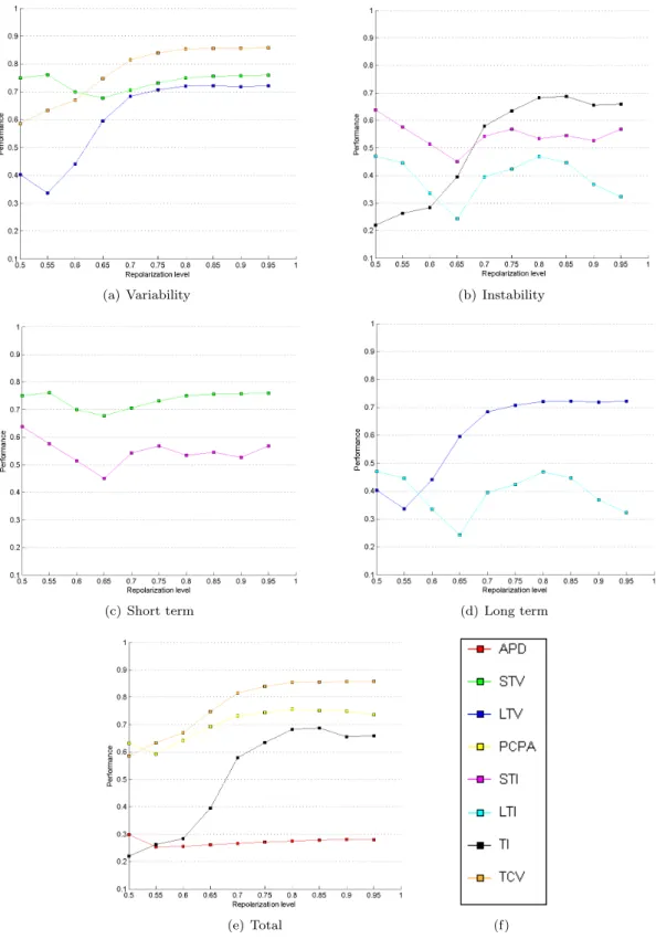
In order to get a better understanding of the influence of the repolarization level on the performance, Figure 6 shows the performance of the BVR measures for different repolarization levels. This figure clearly illustrates the

Figure 6: Performances

observations made above. Moreover, it also shows that STV, PCPA and TCV are reasonably robust measures. If the repolarization level decreases, less variability will be present in the APs. Therefore, the performance of almost all measures decreases for low repolarization lev-els. However the decrease of STV, PCPA and TCV is less significant than that of TI and LTV. The ’oscillat-ing’ behaviour of STI and LTI is probably due to the limited number of samples. Different elements of Figure 6 can be found in appendix C for easier comparison.

The measures described in section 2.3 all use action potential durations as their input data. In order to an-alyze if this is a good choice, the statistical comparison described in section 3.1 was applied to the same BVR measures with AP area as input data (the area under an AP in mV·s). The results in Table 2 show that action potential duration clearly outperforms area as input for the different BVR measures.

Performance APD 0.324 STV 0.516 LTV 0.517 PCPA 0.192 STI 0.549 LTI 0.171 TI 0.397 TCV 0.427

(7)

4.2

K-fold crossvalidation

The k-fold crossvalidation test is performed to verify the hypothesis in the statistical comparison that BVR values come from a normal distribution. The mean and stan-dard deviation of the performances after 10 runs of the k-fold crossvalidation procedure are shown in Table 3. Repeated execution of this procedure is necessary since the data set has to be randomized in order to divide the set in a test and training part. Although there is

NN µ±σ Statµ±σ APD 0.500±0.141 0.492±0.107 STV 0.767±0.035 0.475±0.176 LTV 0.625±0.090 0.608±0.056 PCPA 0.817±0.053 0.517±0.156 STI 0.433±0.086 0.475±0.112 LTI 0.450±0.098 0.433±0.117 TI 0.650±0.086 0.633±0.105 TCV 0.767±0.066 0.733±0.077

Table 3: Results for the nearest neighbour (NN) and statistical (Stat) classifiers

a significant standard deviation, the general scores are comparable to the statistical performances presented in Table 1. Moreover, the results of the two classifiers are comparable for most BVR measures. It is expected that, as the number of samples increases, these numbers will become increasingly similar and will converge to a value that is similar to the statistical performance.

4.3

Application of results

It must be emphasized that the values in Table 1 should not be used as hard thresholds to assess the level of ar-rhythmogenic behaviour. BVR values differ from in-dividual to inin-dividual and from cycle length to cycle length. Moreover, a BVR value that indicates arrhyth-mia in one individual can have a normal result in an-other. However, there are several possibilities to use the information in this table in such a way that one can gen-eralize beyond this set, although the results might not be applicable to all data.

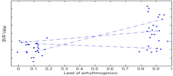
If arrhythmia is seen as a process with a continuous measure for intensity (with 0 being non-arrhythmogenic and 1 being extremely arrhythmogenic) it is possible to use the information in a set with known data, to-gether with information about the change of the BVR of a new sample, to give an indication about the level of arrhythmia. Figure 7 shows BVR versus the level of arrhythmia for a hypothetical data set. Each indi-vidual is represented by two points: a BVR value in the non-arrhythmogenic situation and a BVR value in the arrhythmogenic situation. Although in this research

only a pacing length of 1000 ms is used, it may be pos-sible to find a relation between cycle length and BVR. If such a relation is found, AP series from different cycle lengths can still be compared and the application be-comes more universal. The paths between arrhythmo-genic and non-arrhythmoarrhythmo-genic behaviour capture infor-mation about the development of the BVR with respect to the increasing level of arrhythmia. For a new

indi-Figure 7: Hypothetical data set (only 3 paths illustrated)

vidual, the BVR value and its development over time, can be compared to the paths in the data set to give an indication of the level of arrhythmia. In order to give a reliable indication, it is important that a good distinc-tion between the two sets can be made, in terms of BVR values. This is exactly what is expressed in the per-formance measure described in section 3.1. Also, note that it is not necessary to have an exact measure for the level of arrhythmia. In this research just two levels were used: non-arrhythmogenic and completely arrhythmo-genic. Finally, even the assumption that arrhythmia has a continuous measure for intensity is not essential for the process described above, since thresholding can be used to create different categories.

5

Mathematical cell model

A mathematical cell model can help to elucidate certain aspects of repolarization in general and BVR in partic-ular, by providing insight in the effects that changes in ionic currents have on repolarization. Knowledge about these mechanisms could result in additional control of BVR in experimental conditions, for example by phar-macological intervention. Since BVR is linked to ar-rhythmogenic behaviour (as described in section 4.3), this could be an alternative approach to prevent or treat arrhythmias [17]. Besides, mathematical models make it possible to analyze repolarization aspects that otherwise would require difficult or expensive experiments.

This section first gives an introduction to the mathe-matical cell model for canine ventricular myocytes devel-oped by Hund and Rudy and then describes its relation to the different BVR measures discussed in section 2.3.

(8)

5.1

Cell model

The Hund-Rudy dynamic cell model (HRd model) [8] is an extension of the Luo-Rudy model [9, 10] which was mainly based on guinea pig ventricular cell data. The model is based on an ordinary differential equation controlling the membrane potential:

dV

dt =−

1

Cm

(Ii+Ist) (28)

where d_dV_t is the derivative of the membrane potential,

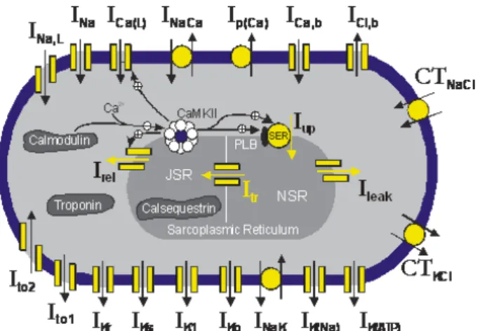
Cmis the membrane capacitance,Istis the stimulus cur-rent andIiis the sum of all currents caused by the flow of different ions. The flow of these ions depends on volt-age gated channels and other mechanisms such as ion exchangers. The gating variables can be determined by a system of coupled differential equations. Figure 8 gives a schematic overview of the model.

Figure 8: Hund-Rudy model schematic [8]

5.2

Adaptations

The physiological fundament of the HRd model is left untouched. However, the following adaptations are made to the original MATLABR _{implementation [11]:}

• The possibility to to block or stimulate certain ionic currents (IKr, IKs, etc.) by adjusting the conduc-tancy.

• The possibility to vary the cycle length and stimulus current after a specified number of APs, thereby facilitating research on pause dependent behaviour [15].

• Variable extracellular conditions ([K+_]

o,[N a+]o and [Ca2+_]

o) to match the experimental conditions. With these adaptations, it is possible to compare the data generated by the HRd model to the experimental data presented in section ’Test method’.

5.3

BVR in the HRd model

The data described in section 3 represent empirical sin-gle cell recordings of canine sinus rhythm cells treated with anIKr blocker. The standard buffer solution con-sisted of 145 mM NaCl, 5.4 mM KCl and 1.8 mM CaCl2.

Recordings were taken using a pacing length of 1000 ms. The HRd model was set up with these parameters (ta-ble 4). The simulation generated 100 APs with these

[K+_] o = 5.4 [N a+_] o = 145 [Ca2+_] o = 1.8 Cycle length = 1000 ms Is = -80 mV Table 4: HRd simulation settings

settings under normal conditions (no blockers active). The last 30 of these 100 APs were used to measure the values of the different BVR measures. This was done in order to avoid possible start-up artifacts. The val-ues are shown in Table 5. It is clear from this table

HRd Value APD 0.2168 STV 0.0002 LTV 0.0003 PCPA 0.0000 STI 0.0002 LTI 0.0102 TI 0.0102 TCV 0.0002

Table 5: HRd results under normal conditions

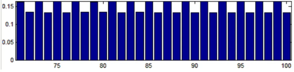
that the HRd model does not contain any form of BVR. The small values in the table result from round off er-rors due to the resolution of the time calculations. This observation is further illustrated in appendix D where sample output of the model is shown. The only indica-tion of BVR under normal condiindica-tions can be found by adjusting the cycle length to 250 ms. Under these condi-tions the APs generated by the model show alternating behaviour (successive short and long action potentials), thereby resulting in a significant value for some BVR measures. This alternation can be seen in figure 16. Al-though in this model it is too regular to be a realistic form of BVR, alternation can be perceived at short cy-cle lengths in empirical data. To further illustrate the dependence on cycle length, figure 9 shows the values of two BVR measures for different cycle lengths. Although it is not apparent from these BVR values, there is cou-pling between successive APs in the HRd model. This can be seen if, similar to the empirical data, the rapid

(9)

Figure 9: STV and LTV at different cycle lengths

activating potassium current (IKr) is blocked. Figure 10 shows the intracellular potassium concentration ([K+_]

i) for different levels ofIKrblock. As expected when

block-Figure 10: [K+_]

i under different levels ofIKr block

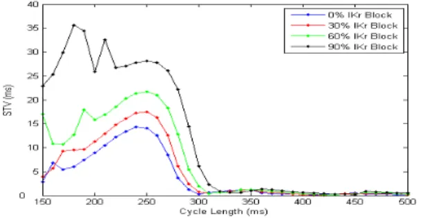
ing an outgoing current, the intracellular potassium con-centration increases over time ifIKris blocked. This has some effect on the alternation that occurs at the short cycle lengths, as can be seen in figure 11. However, this

Figure 11: STV versus cycle length for different levels of

IKr block

figure also illustrates that there is still no form of BVR at the longer cycle lengths, for any level ofIKr block.

With these limitations in the HRd model, it is cur-rently impossible to relate the BVR values of the empir-ical data found in section ’Test results’ to the different ionic parameters that make up the APs.

6

Conclusions &

Recommendations

BVR is a relatively new approach to arrhythmia predica-tion that appears to have a lot of potential. Especially in combination with mathematical cell models it may provide new insights in the different ionic processes that influence BVR in single cell environments. Once more knowledge about this environment is obtained, it may be possible to use this knowledge in new anti arrhyth-mic drug treatments as well as help to better analyze the complexity in multi cell environments. This can be seen a the process of explaining macroscopic properties through the understanding of microscopic behaviour.

6.1

Conclusions

Based on results in this research, which agree with find-ings by others, it can be said that BVR appears to be an accurate approach to predict the incidence of arrhythmo-genic behaviour. However, due to the general definition of BVR presented here (equation 1), it must be empha-sized that not all BVR measures are equally successful. Thomsen et al. [13], among others, observed that action potential duration is not a successful indicator. This is supported by the comparison in this research, although only a limited number of samples are used. However, with the general framework designed here it is relatively easy to extend this data set. In general, it appears that Poincar´e plots adequately capture both short and long term information from the AP series. Of the measures based on this technique, STV, PCPA and TCV can make the best distinction between the two classes. The high performance of TCV can be explained by the fact that it is a combination of three positively correlated measures. This results in a larger difference between the classes.

Attention must be paid to the application of the re-sults presented here. BVR values cannot easily be sepa-rated from the individual cells they belong to. However, by comparing the development of BVR over time to a suitable information set, valuable information about the level of arrhythmogenic behaviour can be obtained.

With respect to the Hund-Rudy dynamic cell model, the main conclusion is that this model is currently not ca-pable of simulating realistic BVR properties. A stronger coupling/relation between the different ionic currents and between consecutive APs appears to be necessary in order to get this behaviour.

6.2

Recommendations

Although some questions are answered in this research, many more have arisen. Some of these questions are stated below and can serve as starting points for further research:

(10)

• Is the current comparison of BVR measures com-plete and how can combined measures such as TCV be used in arrhythmia prediction?

• How can the performance of measures based on Poincar´e plots be explained and are there additional techniques that can be used?

• What adaptations have to be made to the HRd model to incorporate realistic BVR properties? • How can experimental BVR properties and

mor-phologies of APs be related to the ionic mecha-nisms?

• Is it possible to relate BVR values to the cycle length of the recording?

These questions can provide further insight to the gen-eral question of ”What causes BVR and how can BVR be controlled?”

References

[1] American Cancer Society, Inc. (2001). Cancer facts and figures. Surveillance Research.

[2] American Heart Association, Inc. (2000). Guide-lines 2000 for cardiovascular resuscitation and emergency cardiovascular care. Circulation, Vol. 102(8), pp. 11–384.

[3] Brennan, M, Palaniswami, M, and Kamen, PW (2001). Do existing measures of Poincar´e plot geometry reflect nonlinear features of heart rate variability? IEEE Transactions on Biomedical Engineering, Vol. 48(11), pp. 1342–1347.

[4] Can, I, Aytemir, K, Kose, S, and Oto, A (2002). Physiological mechanisms influencing cardiac re-polarization and QT interval. Cardiac Electro-physiology Review, Vol. 6(3), pp. 278–281. [5] Cohen, TJ (2005). Practical Electrophysiology,

Chapter 1. HMP Communications.

[6] Delmar, M (2006). Cell to bedside: Bioelectricity.

Heart Rythm, Vol. 3(1), pp. 114–119.

[7] Hondeghem, LM, Carlsson, L, and Duker, G (2001). Instability and triangulation of the ac-tion potential predict serious proarrhythmia, but action potential duration prolongation is antiar-rhythmic. Circulation, Vol. 103, pp. 2004–2013. [8] Hund, TJ and Rudy, Y (2004). Rate

depen-dence and regulation of action potential and cal-cium transient in a canine cardiac ventricular cell model. Circulation, Vol. 110, pp. 3168–3174. [9] Luo, CH and Rudy, Y (1994a). A dynamic

model of the cardiac ventricular action potential, i. simulations of ionic currents and concentration

changes. Circulation Research, Vol. 74(6), pp. 1071–1096.

[10] Luo, CH and Rudy, Y (1994b). A dynamic model of the cardiac ventricular action potential, ii. afterdepolarizations, triggered activity, and po-tentation. Circulation Research, Vol. 74(6), pp. 1097–1113.

[11] RudyLab, (Washington University St Louis) (2005). The hund-rudy dynamic (hrd) model of the canine ventricular myocyte. http://rudylab.wustl.edu/research/cell/ methodology/cellmodels/HRd/HRD%20on%20 the%20web/HRD%20Introduction.html.

[12] Thomsen, MB, Verduyn, SC, Stengl, M, Beek-man, JDM, Pater, G de, Opstal, J van, Volders, PGA, and Vos, MA (2004). Increased short-term variability of repolarization predicts d-sotalol-induced torsades de pointes in dogs. Circulation, Vol. 110, pp. 2453–2459.

[13] Thomsen, MB (2005). Beat-To-Beat Variability of Repolarisation and Drug-Induced Torsades de Pointes in the Canine Heart. Ph.D. thesis, Uni-versiteit Maastricht.

[14] Linde, H van der, Water, A van de, Loots, W, Deuren, B van, Lu, HR, Ammel, K van, Peeters, M, and Gallacher, DJ (2005). A new method to calculate the beat-to-beat instability of QT du-ration in drug-induced long QT in anesthetized dogs. Journal of Pharmacological and Toxicolog-ical Methods, Vol. 52, pp. 168–177.

[15] Viswanathan, PC and Rudy, Y (1999). Pause induced early afterdepolarizations in the long qt syndrome: a simulation study. Cardiovascular Research, Vol. 42, pp. 530–542.

[16] Volders, PGA, Vos, MA, Szabo, B, Sipido, KR, Groot, SHM de, Gorgels, APM, Wellens, HJJ, and Lazzara, R (2000). Progress in the under-standing of cardiac early afterdepolarizations and torsades de pointes: time to revise current con-cepts. Cardiovascular Research, Vol. 46, pp. 376– 392.

[17] Weiss, JN, Garfinkel, A, Karagueuzian, HS, Qu, Z, and Chen, PS (1999). Chaos and the transi-tion to ventricular fibrillatransi-tion : A new approach to antiarrhythmic drug evaluation. Circulation, Vol. 99, pp. 2819–2826.

[18] Zheng, Z, Croft, J, Giles, W, and Mensah, G. (2001). Sudden cardiac death in the United States, 1989-1998. Circulation, Vol. 104, pp. 2158–2163.

(11)

A

Construction of Poincar´

e plot area

(a) Poincar´e plot (b) Poincar´e plot with convex hull and arrows indicating path between two points on the convex hull

(c) All areas that are substracted from the area of the convex hull

Figure 12: Three phases in the calculation of the Poincar´e plot area

B

Data set

The BVR values for the AP series that are used in this research are presented below:

i APD(ms) STV(ms) LTV(ms) PCPA(s2₎ _STI _(ms) _LTI_(ms) _TI_(ms) _TCV

1 398 25.4 16.8 4.8·10−3 _22.6 _15.7 _36.8 ₉_._2·10−4 2 460 20.5 53.2 9.5·10−3 _06.0 _13.5 _17.9 ₁_._7·10−3 3 374 11.8 15.4 1.7·10−3 _09.3 _18.9 _28.8 ₂_._6·10−4 4 355 19.0 43.6 1.5·10−2 _10.4 _26.6 _36.4 ₁_._6·10−3 5 379 23.2 30.0 1.3·10−2 _13.4 _26.9 _34.0 ₁_._4·10−3 6 438 25.6 27.5 9.7·10−3 _18.0 _24.5 _34.3 ₁_._3·10−3

Table 6: Arrhythmogenic test set

i APD(ms) STV(ms) LTV(ms) PCPA(s2₎ _STI _(ms) _LTI_(ms) _TI_(ms) _TCV

1 409 17.6 16.1 4.0·10−3 _12.5 _22.7 _26.1 ₄_._9·10−4 2 403 06.9 06.1 7.3·10−4 _06.7 _18.9 _21.2 ₇_._1·10−5 3 353 08.3 08.5 1.0·10−3 _05.8 _16.2 _18.3 ₁_._1·10−4 4 328 09.4 15.0 3.0·10−3 _04.6 _20.2 _26.1 ₂_._1·10−4 5 298 05.2 07.0 4.6·10−4 _04.6 _15.0 _17.0 ₄_._9·10−5 6 426 12.5 18.6 4.0·10−3 _09.7 _15.0 _17.8 ₃_._7·10−4

(12)