Do Energy Prices Influence Investment in Energy Efficiency?
Evidence from Energy Star Appliances
Grant D. Jacobsen
∗University of Oregon
September 2015
Published:
Journal of Environmental Economics and Management, 74 (2015) 94-106
Abstract
I examine whether electricity prices influence the likelihood that consumers purchase high efficiency appliances by using state-year panel data on electricity prices and the proportion of sales of new appliances that involve high efficiency “Energy Star” models. I find no evidence that electricity prices affect the propensity for consumers to choose high efficiency appliances. Point estimates are extremely small and precisely estimated. The findings suggest that price-based energy policies may be limited in the extent to which they increase investment in residential energy efficiency, which has been considered one of the lowest cost opportunities for reducing carbon emissions.
JEL Codes: Q3, Q4, D1
Keywords: energy efficiency; Energy Star; appliances; electricity prices; energy efficiency gap; energy efficiency paradox
∗Post: 1209 University of Oregon, 119 Hendricks Hall, Eugene, OR, 97403-1209, Tel: (541) 346-3419,
Fax: (541) 346-2040, Email: gdjaco@uoregon.edu. I am thankful for helpful comments received at the Oregon Resource and Environmental Economics Workshop and from two anonymous referees. This research was supported by the University of Oregon’s Summer Research Grants Program.
1
Introduction
The negative externalities that are associated with energy consumption, often in the form of emissions of greenhouse gases and other pollutants, provide the basis of numerous poli-cies aimed at reducing energy consumption. Price-based polipoli-cies, such as an emissions tax or cap-and-trade program, provide an appealing avenue by which to induce conservation because the increase in energy prices provides incentives for a broad set of economic actors to find ways to reduce their consumption. For example, a substantial literature on the price elasticity of demand for electricity has found that households reduce consumption in the face of elevated prices.1
The way in which households reduce consumption is likely to have important im-plications for the welfare effects of price-based policies. A large body of literature on the “energy efficiency gap” (sometimes called “energy efficiency paradox”) has presented evidence that consumers substantially under-invest in energy efficiency and that many in-vestment opportunities exist that offer high rates of return in the form of reduced energy bills.2 In the presence of unexploited opportunities for high-return investments in energy
efficiency, the loss in consumer surplus from a price-based policy may be very low or even negative if consumers respond to policy-induced increases in prices by purchasing high efficiency appliances and equipment. In contrast, if consumers respond by changing their consumption of energy services, for example by adjusting the thermostat, then consumers are likely to experience a more significant loss in surplus (albeit one that may be justified based on the simultaneous reduction in social damages).
While the relationship between energy prices and investment in energy-using durables has important implications for policy, research in this area is surprisingly sparse, especially within the context of electricity consumption. Of the studies that exist, most have been
1See Espey and Espey (2004) for a meta-analysis of the price elasticity of demand for residential
elec-tricity. Kahn et al. (2014) present related evidence on the importance of energy costs in the commercial sector.
2Gillingham and Palmer (2014) and Allcott and Greenstone (2012) provide recent surveys on the
energy efficiency gap. Both papers suggest that the energy efficiency gap has likely been overstated in many studies (especially in consulting reports from McKinsey and Co.), but that the gap is also not zero.
based on cross-sectional datasets. The earliest notable studies followed the energy crises of the 1970s and early 1980s. Hausman (1979) provides a discrete-model of consumer choice across types of air-conditioners based on 65 observations and Dubin and McFadden (1984) provides a similar analysis of consumer choice of heating systems. Both studies, as well as Gately (1980), find that households value but substantially discount future energy costs when purchasing appliances.
Perhaps prompted by heightened concerns related to climate change, there has been renewed interest among researchers regarding consumer adoption of electricity-using durables in recent years.3 Rapson (2014) develops a structural model of demand for air-conditioners and finds evidence that consumers value the stream of future savings provided by high efficiency units. Houde (2014) develops a structural model of the U.S. refrigerator market and finds that consumers respond to both energy costs and efficiency labels, though substantial heterogeneity in the nature of the response exists across house-holds. The key distinction of the present study is that it is based on panel data, whereas the earlier studies are both based primarily on cross-sectional variation in prices. Rapson (2014) analyzes cross-sectional variation in the prices faced by households observed in the Residential Energy Consumption survey, where average prices are computed based on a household’s total electricity consumption and expenditures. Houde (2014) links sales data from a major retailer to average electricity price data (at both the state and county level) based on the zip code of the store where the purchase was made.
In this paper, I employ an advantageous yet underexploited dataset to provide new evidence on the relationship between energy prices and investment in energy efficiency. In particular, I evaluate the relationship between state electricity prices and the percentage of sales of new appliances that involve high efficiency “Energy Star” models using state-year level panel data on electricity prices and appliance sales patterns for the period from
3There has also been renewed interest in the effectiveness of policies designed to promote efficiency.
For example, Jacobsen and Kotchen (2012) show that energy efficiency standards for new buildings (“energy codes”) are effective at reducing energy consumption and Jacobsen (in press) shows how energy codes could be designed to prioritize reduced consumption of energy types with large social damages.
2000 to 2009. The advantage of exploiting panel variation is that I can control for time-invariant differences across regions, such as differences in demographics, economics, and consumer preferences, which are difficult to fully control for in a cross-sectional setting. I find little evidence of a relationship between electricity prices and the market share of Energy Star appliances. The point-estimates are very small in magnitude and are precisely estimated. The finding is consistent across different types of appliances and robust to both fixed effects and first-difference specifications, as well as specifications that allow for lagged instead of contemporaneous price effects and specifications that instrument for electricity price changes using variation in natural gas prices.
While the finding that consumers do not respond to energy prices when choosing appliances seems inconsistent with simple models of utility maximization, other studies have documented results in various settings that foreshadow such a finding. Allcott and Taubinsky (2013) implement a field experiment to study the effect of presenting retail shoppers with information about the energy costs associated with different types of light bulbs.4 They find that the availability of information on energy costs does not have
a statistically significant effect on purchase patterns. Kahn and Kok (2014) conduct a hedonic study of the price premium for green homes, which typically have high levels of energy efficiency. They find little evidence that the price premium for a green home increases when there are elevated energy prices.5
In addition to being hinted at by earlier empirical studies, the lack of a response is also consistent with more nuanced theoretical models of consumer behavior in the
4Note that Allcott and Taubinsky (2013) differs from the present study because their focus is primarily
on information. In particular, they examine how information on the expected energy costs of each model (which varies by model due to the differing levels of energy efficiency) has an effect on consumer decision-making, as opposed to how changes in energy prices affect consumer decisions.
5More generally, there are numerous examples of unconventional consumer behavior within the
resi-dential electricity setting. Jessoe et al. (2014) find that households decreased their energy consumption
in response to a shift to time-of-use pricing that represented a pricedecrease. Jessoe and Rapson (2014)
present strong evidence of habit formation in residential energy consumption. Jacobsen et al. (2012) find evidence of moral licensing in the context of residential electricity consumption and green electricity programs. Gromet et al. (2013) presents laboratory-based evidence that prominent energy labels can lead to perverse outcomes for consumers with conservative ideologies. Fowlie et al. (2015) present ex-perimental evidence that households have very low take-up rates of “weatherization” retrofits even when the expected benefits are sizable and the monetary benefits are zero.
context of energy efficiency. Using theory and evidence, Sallee (in press) shows that it is rational for consumers to ignore energy efficiency in many settings because assessing the value of energy efficiency often requires time and effort and because energy efficiency is unlikely to be a pivotal feature when consumers have strong preferences about other product attributes. Similar arguments can be applied in the context of this study. Given the complexities of electricity usage and billing, most consumers are likely to find it difficult to evaluate how energy prices influence the returns to energy efficiency and such knowledge, even if acquired, may be unlikely to influence their choice of product given the many different features of appliances.
Finally, while the finding that appliance sales patterns do not respond to state en-ergy prices deviates from previous studies on enen-ergy prices and appliance choice, it is perhaps what one might predict in light of the labeling scheme used for appliances. In particular, yellow “EnergyGuide” labels are federally required for major appliances in the United States and provide information to consumers on the estimated yearly energy costs associated with different models of appliances. The energy costs displayed on the label are based on national energy prices. EnergyGuide labels disclose that the costs that are displayed are based on national prices, so consumers could potentially recognize that the information presented needs to be adjusted for regional prices, but such a calculation is likely to take time and effort and consumers may instead simply make decisions based on national average costs, or ignore the labels and energy costs altogether.6
This paper primarily contributes to an understanding of consumer behavior within the residential electricity setting. However, the general topic of the relationship between energy prices and consumer choice applies to other settings, most notably that of au-tomobile choice. Several papers have examined how demand for vehicle fuel efficiency depends on gas prices.7 Busse et al. (in press) find that consumers take full account of
6Because there is no spatial variation in the energy costs displayed on EnergyGuide labels, I cannot
test whether consumers are responding to the labels in my empirical setting. I discuss the interplay between labels and prices further in the conclusion, including some recent work in this area by Davis and Metcalf (2014).
future energy costs where making automobile purchases. In contrast, Alcott and Wozny (in press) find evidence that consumers somewhat undervalue future energy savings; ap-proximately trading off $1 in discounted future energy costs for only $0.76 in upfront savings. This paper is similar to these recent studies in that is uses panel data and re-duced form techniques to evaluate the relationship between energy prices and investment in energy efficiency. The novelty of the present paper is that I study the phenomenon in the setting of electricity consumption, a setting that has been more overlooked in the recent literature despite being of equal policy importance.8,9 The collective implication
from these studies and the present one is that consumer investments in efficiency are sensitive to prices when purchasing cars, but not household appliances. Two potential explanations for the contrast in findings are that gasoline prices are more salient than electricity prices and that the purchase of an automobile has a larger impact on current and future expenditures than the purchase of any one appliance, which leads consumers to approach the purchase more carefully.
This paper also contributes to the literature on consumer behavior and eco-labels, which are typically third-party certifications that indicate that a product has been pro-duced or operates in an environmentally-friendly manner. The majority of this litera-ture has focused on consumer willingness to pay for eco-labels.10 Newell and Siikamaki
(2013), Walls, Palmer, and Gerarden (2013) and Houde (2014) each present evidence that consumers have a high willingness to pay for Energy Star certification, and that this willingness-to-pay seems to exceed what can be justified strictly by energy savings. The present study complements these previous studies by implicitly testing whether willingness-to-pay for products with the Energy Star label changes substantially when energy prices change. The fact that Energy Star market share does not respond to price taxes.
8Electricity generation currently produces more greenhouse gas emissions than the transportation
sector in the U.S. (EPA, 2014a).
9There are also relatively few recent studies on how energy prices influence efficiency in the industrial
sector. Linn (2008) provides one of the few available studies, showing that manufacturing plants appear to be built with lower energy intensities during periods when energy prices are elevated.
10Examples, other than those mentioned directly in the text, include Brouenen and Kok (2011), Ward
changes suggests that consumers value Energy Star products for reasons other than simple financial incentives.
The remainder of the paper proceeds as follows. In section 2, I describe the data sources. Section 3 outlines the methodology. Section 4 presents the results. In section 5, I discuss the implications of the findings for policy, describe some of the limitations of the analysis (especially with respect to the coarseness of the dependent variable) and conclude the paper.
2
Data
The outcome of interest in this paper is the propensity for consumers to purchase high efficiency goods as measured by the percentage of sales of new appliances that involve high efficiency “Energy Star” models. Energy Star is a labeling program provided by the U.S. Environmental Protection Agency (EPA) that helps consumers easily identify high efficiency appliances. In order for a product to be designated as an Energy Star appliance, it must meet a number of requirements set forth by the EPA, the most important of which is that it must meet a certain standard for energy efficiency, which is often based on improvements over the minimum efficiency level required by federal regulations. For example, Energy Star refrigerators must be 20 percent more efficient than the minimum federal standard. In addition to being used for appliances, Energy Star labels are also used for electronics, new homes, commercial buildings, and industrial plants.
It should be noted that federal efficiency standards and Energy Star certification standards are based on product attributes.11 Maximum allowable levels of energy
con-sumption for a product under either type of standard vary by size categories and other design features (e.g., whether a refrigerator-freezer is a side-by-side vs bottom freezer unit). Because Energy Star certification standards vary by attribute, Energy Star cer-tification does not perfectly correlate with a product’s overall energy consumption. For
11See Houde and Aldy (2014) for an examination of how attribute-based policies influence consumer
example, a large Energy Star labeled refrigerator may use more energy than a small non-labeled unit. Due to the nature in which Energy Star certifications made, this paper cannot provide a complete evaluation of how appliance purchase patterns with respect to energy respond to price changes. Nonetheless, Energy Star products still provide an interesting example in which to evaluate whether consumers respond to prices change by seeking out higher-efficiency products because Energy Star provides one of the most salient signals of high-efficiency available to consumers.
Annual data on the Energy Star share of new sales in different appliance markets for each state were obtained from the EPA’s Energy Star web page (EPA, 2014b). The data cover the period from 2000 to 2009 and include information on the share of sales that were Energy Star products for each of four major appliances: air-conditioners, clothes washers, dishwashers, and refrigerators. Data are aggregated based on proprietary sales records from Energy Star national retail partners, which are retailers that agree to carry and market Energy Star products, and represent approximately 60 percent of the total retail market for appliances. The dataset effectively represents a balanced panel with 200 cross-sectional identifiers (one each for each combination of state and appliance type), ten time-series units (one for each year in the sample), and 2000 total observations.12
The sales data were matched to annual data on average state residential electricity prices from the Energy Information Administration (EIA, 2014a). Analysis of price effects is complicated in the electricity setting because marginal prices and average prices often differ for electricity due to increasing block rate pricing. I employ average prices because recent research indicates that consumers are primarily responsive to average electricity price in the residential sector (Ito, 2014). Measurement error is a related concern because the average price that is experienced by a household depends on its level of consumption under block rate pricing. This feature can lead to substantial measurement error if there
12Data from other appliance types or for more recent years are not available. While there is some
measurement error in the aggregated market share variable recorded in the data because some retailers may not report in certain time periods, this measurement error should not lead to bias in the analysis because market share is the dependent variable in the regression models.
is a difference in the unit of analysis and the level at which price is measured (e.g., when a household is linked to state average electricity prices). All variables in the data used for the analysis are measured at the state level, which partially mitigates concerns about measurement error.13 I discuss the issue of measurement error further in Sections 3 and
4.
For use as control variables in certain specifications, I obtained and merged annual state-level data on average residential natural gas price, income per capita, and rebate incentives offered by utilities from the State Energy Data System (EIA, 2014b), the Bureau of Economic Analysis (BEA, 2014), and Datta and Gulati (2014), respectively. For use in instrumental variable models, I also obtained and merged data on the average price of natural gas sold to electricity providers in each state’s primary North American Electric Reliability (NERC) region and data on the share of electricity generated through natural gas in 2000 in each state’s primary NERC region from the EIA (2014b) and the EPA (2002), respectively.14 Electricity price, residential natural gas price, income
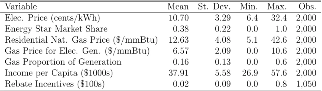
per capita, average rebate incentives, and natural gas price for electric generation were adjusted for inflation using the national consumer price index and 2009 as the index year. Summary statistics for key variables are presented in Table 1. The average electricity price over the sample is about 10 cents/kWh. Energy Star appliances comprise about 40 percent of the market. There is substantial variation in both variables as indicated by the standard deviations and ranges for each variable. The average residential natural gas price during the sample is about $13 per mmBtu and the mean income per capita is close to $38,000. The average natural gas price for electric power is about $7 per mmBtu. The typical state is located in a NERC region where about 16 percent of electric power is generated through natural gas.
13Measurement error is not fully addressed by using state-level data. For example, if the pool of
individuals purchasing appliances are located in areas of a state that do not reflect average state electricity prices, and consumers respond to local as opposed to state prices (as indicated in Ito (2014) and Busse et al. (in press)), then measurement error will remain a problem.
14As I describe further when presenting the instrumental variable results, states were linked to NERC
regions because of the interconnectivity of wholesale electricity markets across state borders. For states that overlay multiple NERC regions, each state was matched to the NERC region that contained the largest share of the state’s generation (as reported in EPA (2002)).
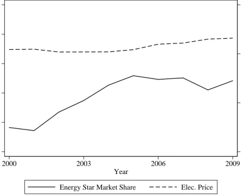
Figure 1 displays trends in national averages for electricity prices and Energy Star market share (henceforth “ES Market Share”). Mean electricity price levels are relatively stable across the years in the sample. In contrast, ES market share is generally increasing. Increasing ES market share is reflective of the increasing levels of efficiency throughout the U.S. economy as energy use per capita and energy use per dollar of GDP have both declined substantially in the past decade (EIA, 2014c).
3
Methodology
Figure 1 is useful for initially characterizing the data, but it is not especially helpful for evaluating the effect of electricity prices on ES market share because other factors related to the development or adoption energy efficient technologies that influence national trends in Energy Star appliances could falsely suggest or mask a relationship between electricity prices and ES market share. A better approach for evaluating the effect of electricity prices on the purchase of high efficiency appliances is to compare different patterns across states. A state-level analysis has the benefit of being able to control for nation-wide trends in ES market share that could be driven by decisions made by appliance retailers or producers related to product inventory, pricing, or development.
An additional benefit of comparing state trends is that while there is only minimal variation in the average national price across the sample years, there is substantial within state price variation. I present information on electricity price variation by state in Table 2. Forty-four of the 50 states experienced at least a 10 percent difference between their minimum and maximum price observed in the sample. There is also substantial differences in the scope of price variation across states. For example, the 10 states with the smallest difference between their minimum and maximum observed prices had a mean price difference of .76 cents/kWh, whereas the 10 states with the largest difference had a 5.6 cent/kWh price difference.15 These differences are non-trivial, as each 1 cent/kWh
15Measured as a percentage, these price differences correspond to a 5.6 percent difference and a 45.8
change in prices corresponds to over $100 in extra annual energy costs based on average residential consumption levels in the U.S.16
One concern with exploiting state-specific variation in prices is that state-specific price changes may only represent temporary deviations from national patterns. In such a case, a rational consumer might disregard regional price changes and instead focus on national prices when investing in energy efficiency. However, the factors that influence electricity prices are likely to generate distinct non-transient changes in regional prices. Most notably, there is substantial variation in the sources of generation used across regions and these differences influence how electricity prices change in response to recent changes in fuel costs.17 The more electricity that a region consumes from a certain source, the more that region will be affected when the price of that fuel changes. For example, changes in natural gas price are unlikely to have as large of an affect in the mid-west, a region which relies heavily on coal and uses very little gas, than in the west and northeast, where generation from natural gas comprises about a quarter or more of total generation. Because the price of the different fuels used for electric generation are not synchronized, these changes in fuel prices should create non-transient changes in electricity prices across regions.18
Empirically, I investigate whether state-specific prices changes (i.e. state price changes relative to changes in national prices) are transient in two ways. First, I examine whether
16Based on the Energy Star savings calculators, which assume a 4 percent discount rate, the average
change in state prices over the sample period (2.3 cents/kWh) corresponds to an additional lifecycle electicity savings from Energy Star units of $244, $14, and $10 for central air-conditioners, dishwashers, and refrigerators, respectively. As a point of comparison, the average price premiums for Energy Star central air-conditioners, dishwashers, and refrigerators are $556, $10, and $20, respectively. Energy Star does not presently provide a calculator for clotheswashers but the savings would likely be similar to those for dishwashers based on the similarities in usage levels.
17While electricity price changes can be driven by several factors, including changes in fuel costs,
required investments in additional generating capacity and transmission, new environmental regulations, and changes in consumption levels, the most significant source of price changes are those from changes in fuel costs, such as changes in natural gas prices. A consulting report from 2001-2006 reported that 95 percent of the changes in costs experienced by utilities was driven by increases in fuel prices and associated increases in the cost of purchased power (Brattle Group, 2006).
18There are no fuel prices for renewables, such as hydropower and wind power, or for nuclear power.
According to data from the EIA from 2003 to 2013, the correlation between the annual average cost of coal and natural gas sold to the power industry (both measured in dollars per mmBtu) are insignificantly
within state price deviations, as measured by the residuals from a regression of state and year fixed effects on electricity price, influence price deviations in the following year. A regression of residual on lagged residual produces a positive and significant coefficient of .61, indicating price changes in one period influence prices in the following period.19
Secondly, I examine whether there is a systematic trend in these residuals across years for each state. If state prices mimic national prices, then there should be no trend in the residuals across years. I find that 64 percent of states have a significant trend in their residuals (42 percent positive, 22 percent negative).20 In sum, the price patterns
observed across states suggest that a rational consumer should be attentive to regional price changes. I further discuss the issue of variation in price patterns later in this section within the context of an estimation procedure designed to explicitly isolate changes in electricity prices tied to recent changes in the price of natural gas.
I estimate the relationship between electricity prices and ES market share using first-difference and fixed effects regression models. The first-first-difference (FD) regression is based on a specification of the form,
∆ ES Market Shareszt =β∆ Elec. Pricest+θ0∆Xst +γzt+szt (1)
where s indexes states, z indexes appliance type, t indexes years, ∆ ES Market Shareszt
represents the change in ES market share in given state for a given appliance type relative to the previous year, ∆ Elec. Pricest represents the change in electricity prices in a given
state relative to the previous year, ∆Xst represents a first-differenced covariate vector
that includes residential natural gas prices and ln(income per capita), γzt is a vector
of appliance-year dummies variables, and szt is an error term. The fixed effects (FE)
regression is based on a specification of the following form,
19The persistence of price changes is likely stronger than indicated by this exercise because the
co-efficient is negatively biased for reasons similar to the dynamic panel data bias described in Nickell (1981).
20These figures are calculated by separately regressing year (measured continuously) on residual for
ES Market Shareszt =αsz+β Elec. Pricest+θ0Xst +γzt+szt (2)
whereαsz represents a vector of state-appliance fixed effects that control for time-invariant
factors within each state’s appliance markets.21 Standard errors are calculated by
clus-tering on state-type in both the FE and FD specifications.
A key feature of both regressions is that they include a vector of appliance-year dum-mies variables, which control for appliance-specific annual time shocks that are expe-rienced uniformly across all states. Key examples of such shocks include changes in appliance prices, inventory, or marketing implemented nationally by retailers, changes in the Energy Star requirements administered by the EPA, and changes in federal rebates or tax incentives. Both specifications also control for time-invariant differences across states, either through fixed effects or first-differencing. Over the sample period, which is only a decade, factors that can be considered as approximately time-invariant include most demographic variables and environmental ideology.
While both the FD and FE models are valuable, the FD specification has the relative advantage of being less sensitive to spurious correlation than the fixed effects regression when the number of cross-sectional units is not large relative to the number of temporal units. Part of the reason that the FD specification is less sensitive to spurious correlation is that any unobservable shock that persistently changed ES market share within a state would be removed by the first-difference from all but one observation in the FD model, but not in the FE model. Regardless, as described in the next section, both models produce similar results.
Factors that vary temporally across states could lead to biased estimates if these factors are correlated with both electricity prices and ES market share because first-differencing and fixed effects only control for time-invariant differences between states. To limit the potential for bias, I control explicitly for two different time-varying factors:
21State-type fixed effects are not included in equation 1 because they are eliminated by
residential natural gas prices and income per capita. The energy variable of primary interest in the regressions is electricity price because the appliances considered in the data are all powered by electricity, however residential natural gas prices could be important if consumers are responding to their total overall utility bill as opposed to just their electric bill. Income per capita is an appropriate control variable given its significance in household budgets.22
One potential time-varying variable of interest that is not included in the analysis is an appliance price variable that represents how appliance prices differ between Energy Star and non-Energy Star models in a given state and year. Detailed data on appliance prices are not available, but the absence of this variable from the analysis will only influence the primary estimates if changes in appliance prices are systematically correlated with changes in electricity prices. Given the national retailers involved in the appliance market and the reputation and branding concerns that many companies have, some form of strategic response by producers or retailers that would drive such a relationship seems unlikely. For example, Sallee (2011) shows that auto manufacturers do not change their prices for efficient vehicles once subsidies are introduced, despite likely being able to appropriate many of the gains. However, even if appliance prices do respond to electricity prices and this response eliminates any increase in the propensity for consumers to choose more efficient appliances, the primary policy implications of this paper are unchanged. While the mechanism may be either consumer inattention or an induced change in appliance prices—and again I think the latter mechanism is unlikely—the end result is the same: prices changes appear to be an ineffective way of increasing uptake of high efficiency appliances.
In specifications that are similar to those described above, I allow for a time-lag with respect to energy prices. If it takes time for consumers to recognize that prices have
22Conte and Jacobsen (2014) provide evidence that demand for “green goods” is influenced by income,
college graduation rates, and liberalism. Over the relatively short period of the sample, it is unlikely that rates of college graduation and liberalism would fluctuate substantially within a state, especially among the adult population.
changed, or if consumer beliefs about future prices depend on historical, as opposed to contemporaneous prices, then lagged effects may be important. I examine specifications that model electricity prices as influencing market share exclusively through a price lag, as well as through both a price lag and a contemporaneous price effect. It is also possible that consumer preferences depend on expectations of future prices. Anderson et al. (2013) present evidence that consumer beliefs about future energy prices are determined by current prices, indicating that this case would be captured by the specifications based on contemporaneous prices.
In addition to the FE and FD models and the three different price specifications, I investigate a variety of additional robustness checks, including the following.
Separate Models for Each Type of Appliance. In order to examine whether the primary
results hold across each type of appliance, I estimate a separate set of results based on samples that are limited to the observations from each type of appliance. These models are identical to those described in the earlier specifications, with the exception that there is no need to index appliance types, so the z index could be dropped from the notation. I also examine separate models for each type of appliance for the robustness checks described below.
Controlling for Rebate Incentives Offered by Utilities. I control for utility rebate
incentives in a set of results using data from Datta and Gulati (2014).23 The main
reason for not controlling for rebate incentives in the primary regressions is that the data on rebate incentives only encompasses the period from 2001 to 2006 and are not available for air-conditioners. In order to most cleanly investigate the extent to which not controlling for rebate incentives potentially biases the estimates, I also present, for purposes of comparison, the results of models that do not control for rebate incentives but that are limited to the observations for which data on rebate incentives are available.
23Following Datta and Gulati (2014), I do not control for state incentives, primarily because state level
incentives typically only last for a few days of the year, especially during the sample period, which pre-dates the introduction of the State Energy Efficient Appliance Rebate Program (implemented through the American Recovery and Reinvestment Act of 2009, which effectively came into force in 2010).
Instrumenting for Electricity Price using Variation in Natural Gas Price and the Share
of Electricity Generated through Natural Gas. I also examine models that instrument for
state electricity price changes using an interaction of the share of electricity in a state’s NERC region that was generated through natural gas in 2000 and the annual price of natural gas sold to power generators in the state’s NERC region.24 These results are
helpful for two reasons. First, the estimates are based explicitly on variation in electricity prices induced by changes in fuel prices, and this sort of price variation may be viewed by consumers as more likely to be indicative of lasting changes in electricity prices than other sources of price variation. Secondly, instrumental variables estimates are helpful in correcting bias from measurement error, which as mentioned previously, can occur due to the block rate pricing schedules used by most electric utilities. In the instrumental variables (IV) models, the first-stage regression takes the following general form,
∆ Elec Price.szt= β∆ Gas Prop. of Gen.s,2000× Gas Price for Elec. Gen.s,t−1
+ θ0∆Xst+γzt+szt, (3)
and the second stage regression is based on the following specification,
∆ ES Market Shareszt =β∆ Elec. Priceˆ st+θ0∆Xst+γzt+szt (4)
where ∆ Elec. Priceˆ stis the predicted value from the first-stage. I also estimate analogous
IV results based on a fixed effects model. Note that in the first stage natural gas price for electric generation is lagged by one year. This lag reflects the delay that utilities face in going through the ratemaking process.25 As mentioned previously, Gas Proportion of
Generation and Gas Price for Electricity Generation are measured at the NERC-level
due to the interconnectivity of the wholesale electricity market. Each state is matched to one of twelve NERC regions. Using NERC-level variation is common in analyses of
24I use data on the generation mix from 2000 (i.e. the beginning of the sample) so that the results are
strictly based on temporal variation over the sample period in natural gas prices, as opposed to temporal variation in both natural gas prices and investments in generating capacity.
25Results are qualitatively similar if natural gas price for electric power is modeled as having a
electricity markets (e.g., Jacobsen, 2014, Paul and Burtraw, 2002) because substantial trading of power occurs across state borders.
Before moving to the results, it should be noted that there are often concerns about price endogeneity in studies of the price elasticity of demand for electricity. The primary concern is that prices and consumption are systematically linked due to block rate pricing. In this paper, the outcome of interest is not electricity consumption, so concerns about endogeneity are minimal. In theory, efficiency investments could reduce demand for a portion of the year in which they are purchased. However, it is likely that any impact on average state electricity prices from efficiency improvements would be near zero because of the low rate of replacement for the appliances under study (due to their long life-spans), the modest improvements in efficiency offered by ES products, and the large number of other components and behaviors that contribute to residential demand.
4
Results
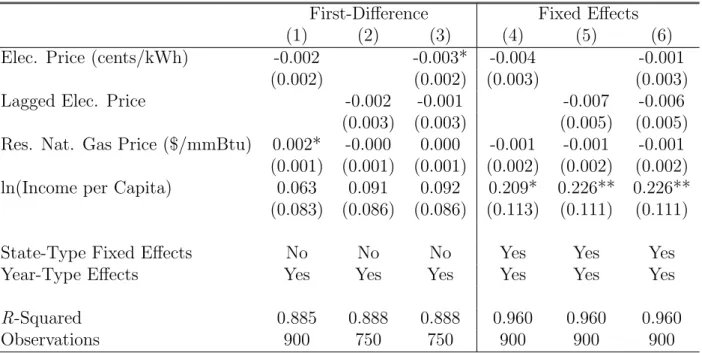
Results for the full sample are reported in Table 3. The first three columns present estimates from FD specifications. The first column allows only for a contemporaneous price effect, the second column allows only for a lagged price effect, and the third allows for both contemporaneous and lagged price effects. Across models, there is very little evidence of a relationship between electricity prices and ES market share. Point estimates are small in magnitude–equal to or less than three-tenths of a percentage point in absolute value in all cases–and the estimates are precisely estimated with standard errors under three-tenths of a percentage point. An analogous set of estimates is presented for the FE specification in the fourth through sixth columns.26 The coefficients on electricity
price are extremely similar to those in the FD specifications. Examining the covariates, there is some modest evidence that natural gas has a positive impact on ES market share
26The number of observations varies across models because observations from 2000 are excluded from
the FD specifications and observations from the first observation in each time-series (after dropping 2000 in the FD specifications) are excluded from the models that include a lagged price variable.
in the FD specifications, but the result does not hold in the FE specification. There is also some evidence that income has a positive impact on ES market share, though the evidence is inconsistent here as well. Overall, it is not surprising to find mixed evidence with respect to the coefficients on the control variables because there are not strong theoretical predictions regarding the direction of the relationship between these variables and ES market share.27 In sum, Table 3 provides evidence across specifications that
electricity prices do not influence consumer adoption of Energy Star appliances.
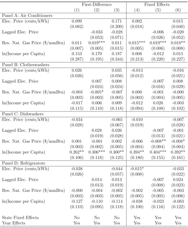
In Table 4, I present results similar to those presented in Table 3 except each model is estimated separately for each type of appliance. Across types of appliances and models there is little evidence of a relationship between electricity prices and ES market share. The coefficients that are reported in column 1, which presents results for perhaps the most preferred specification, are all small in magnitude and two of the four coefficients are exactly estimated at zero after rounding to the tenth of a percentage point. The only coefficient that is consistently significant is the coefficient on the lagged price variable for refrigerators. However, the point estimate takes the opposite sign that would be expected if consumers were rationally responding to increased energy prices. Given the large number of coefficients being tested across Tables 3 and 4, it is not surprising to have one relationship return as statistically significant even in the presence of a null relationship within the population. With respect to the covariates, there is also some evidence that natural gas prices and income per capita are positively associated with ES market share, but the evidence is inconsistent across samples. On net, Table 4 reinforces the findings presented in Table 3; there is little evidence of a relationship between electricity prices and ES market share.
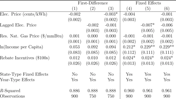
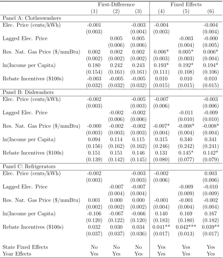
In Table 5, I present results based on the limited sample from 2001 to 2006, excluding air-conditioners, that include rebate incentives as a control variable. Similar to Datta and Gulati (2014), I find evidence that rebate incentives for Energy Star appliances
27The results are qualitatively unchanged if the time-varying control variables are omitted from the
are effective at increasing ES market share in the FE specifications.28 A $100 increase
in average rebate incentives is associated with a 2.4 percentage point increase in ES market share. More importantly, the results in Table 5 also provide little evidence of a relationship between electricity prices and ES market share.29 To shed light on whether
the omission of rebate incentives from other models is likely to lead to bias, I also provide results based on models that exclude rebate incentives using the sample of observations for which rebate incentives are not missing. The results, which are reported in Table 9 (provided in the Online Appendix) are nearly identical to the results in Tale 5, suggesting that the omission of rebate incentives from other models does not produce bias in the primary coefficients.
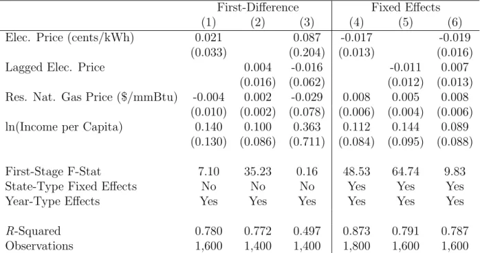
In Table 6, I present instrumental variables estimates based on variation in natural gas prices and the regional power mix (first stage estimates can be found in Table 7 in the Appendix).30 As indicated by the F-statistics, only the results reported in columns 2, 4, and 5 clearly pass weak instrument tests and the other results should be appropriately discounted. While the estimates lose efficiency due to the two-stage procedure, they also fail to show a positive relationship between electricity prices and ES market share. In all the specifications that pass the weak instrument tests, the coefficients are insignificant and the point estimates either small or negative. See Table 10 (provided in the Online Appendix) for IV estimates by appliance types. Results are substantially noisier, but also indicate an insignificant relationship between electricity price and ES market share.
The collective set of results indicates that changes in electricity prices are not posi-tively associated with changes in the market share of Energy Star appliances. The most
28My results are not directly comparable to Datta and Gulati (2014) because Datta and Gulati use
quarterly data and exploit within-year-state variation in the offering of rebates. Quarterly data are not appropriate for the present paper because quarterly variation in electricity prices within a state is generally driven by seasonal fluctuations in consumption levels.
29Table 8 (provided in the Online Appendix) provides results for each type of appliance that control
for rebate incentives. These results also fail to detect a relationship between electricity price and ES market share.
30In specifications based on contemporaneous electricity prices, the lag of the price of natural gas sold
to power providers is used as instrument. In specifications based on lagged electricity price, the twice-lagged price of natural gas sold to power providers is used as instrument. There is a clear and strong relationship between the price of natural gas sold to power providers and residential electricity prices.
straightforward explanation for the observed results is that consumers do not carefully consider electricity costs when purchasing appliances. One alternative explanation is that the results are biased due to measurement error related to block-rate pricing. In particular, if the average electricity price facing purchasers of new appliances differs from the average overall residential electricity price, then the estimates would be subject to a degree of attenuation bias. Two parts of the results run counter to this explanation. First, the IV models, which are not biased by measurement error, also failed to detect a relationship. Second, the near-zero and often negative coefficients that are present across the primary specifications is most consistent with the total lack of a relationship between electricity prices and ES market share, rather than with a relationship attenuated by measurement error, in which case non-zero point estimates would still be expected, as well as ones of a positive sign.
5
Conclusion
This paper provides the first study that I am aware of that has used panel data techniques to examine how electricity prices influence investment in energy-using durables. I find no evidence that increases in electricity prices make consumers more likely to purchase high efficiency Energy Star appliances. The findings suggest there are limitations in the extent when energy prices influence investment in residential energy efficiency.
There are several reasons why the results should not be interpreted as evidence that consumer decisions related to residential energy efficiency are completely non-responsive to energy prices. For one, the outcome variable, ES market share, does not fully character-ize consumer choices related to appliances and energy. As such, I am unable to comment on whether consumers respond to changing electricity prices by purchasing smaller appli-ances, changing the rate at which they upgrade their appliappli-ances, or buying more efficient appliances within the pool of ES-labeled and non-ES-labeled products. I am also unable to comment on how energy prices affect investment in other types of household products
other than those considered in the analysis, such as light bulbs, furnaces, and insula-tion. Additionally, the market data that the outcome is based on represents only about 60 percent of the appliance market, and the results could potentially differ if complete market data were available and employed. Finally, the results in this paper are based on variation in state prices and it is possible that a nation-wide shift in prices induced by a national carbon policy would send a more salient price signal to which consumers might more readily respond.
Fully characterizing how consumers respond to energy prices in an important area for policy design. The extent to which investment in energy efficiency responds to changes in electricity prices has implications for the expected costs of carbon mitigation, especially for price-based policies, and for which types of policies are most cost-effective. If the energy efficiency gap is substantial and consumers fail to respond to price-based incen-tives when investing in energy efficiency, then standards or subsidies may represent the least cost way of reducing energy-related externalities, at least for low levels of emissions reductions. Additionally, if prices are ineffective at promoting investment in energy ef-ficiency, then supply-based policies, such as R&D subsidies, may be necessary to drive meaningful advances in technological innovation.31 R&D subsidies, especially when
ad-ministered upstream, have become increasingly favored in recent years by economists as a means of addressing climate change because they experience fewer problems related to emissions leakage and are often more politically feasible (Fischer et al. 2014).
Given its policy importance, researchers should continue to investigate the relation-ship between energy efficiency and energy prices. It would be particularly helpful to identify how the relationship varies across settings. For example, it would be interesting to evaluate whether household investments in energy efficiency are more responsive to energy prices when households have precise information on energy prices and usage. Re-cent research by Jessoe and Rapson (2014) and Davis and Metcalf (2014) has indicated
31Newell et al. (1999) directly evaluate whether energy prices induce innovation in the context of
energy efficiency and find mixed evidence. Energy prices do not appear to influence the rate of overall innovation. The direction of innovation responds to energy prices for some products but not for all.
that information plays an important role in how prices influence consumer behavior in the energy sector.32 It would also be interesting to examine how consumers respond to
changes in energy prices that are larger than those considered in this study.33 I leave
these and other questions to future researchers.
32Jessoe and Rapson (2014) document that residential energy consumption is more responsive to
short-term changes in energy prices when residences are equipped with in-home displays that provide households with detailed information on usage and expenditures. Davis and Metcalf (2014) present experimental evidence based on hypothetical purchase decisions that designing EnergyGuide labels so that they present information based on state energy prices, as opposed to national prices, would alter consumption patterns for appliances in the United States.
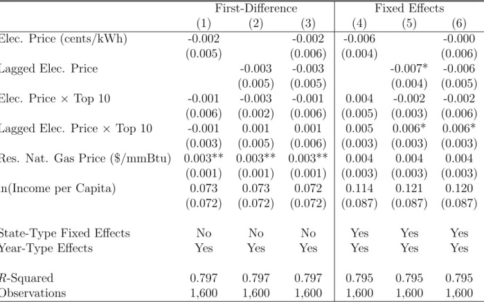
33I provide some evidence on whether larger price changes are more influential by estimating models
that allow for a heterogeneous price effect depending on whether a state was one of the 10 states in the sample that experienced the most variation in electricity prices over the sample period. Even for the states with the most price variation, there was little evidence that prices influenced ES market share (see Table 11 in the Online Appendix).
References
Allcott, H. and M. Greenstone. 2012. “Is There an Energy Efficiency Gap?,” Journal
of Economics Perspectives 26 (1), 3-28.
Allcott, H. and D. Taubinskly. 2013. “The Lightbulb Paradox: Evidence from Two Randomized Experiments,” Harvard University Working Paper.
Allcott, H. and N. Wozny. In press. “Gasoline Price, Fuel Economy, and the Energy Paradox,” Review of Economics & Statistics, in press.
Anderson, S. T., R. Kellogg, and J. M. Sallee. 2013. “What Do Consumer Believe About Future Gasoline Prices?,” Journal of Environmental Economics and Management
66 (3), 383-403.
Brattle Group. 2006. “Why Are Electricity Prices Increasing?,” The Edison Foundation: Washington, DC.
Brounen, D. and N. Kok. 2011. “On the Economics of Energy Labels in the Housing Market,” Journal of Environmental Economics and Management 62 (2), 166-179 Burtraw, D., R. Sweeney, and M. Wells. 2009. “The Incidence of U.S. Climate
Pol-icy: Alternative Uses of Revenues from a Cap-and-Trade Auction,” National Tax
Journal 629 (3), 497-518.
Bureau of Economic Analysis (BEA). 2014. BEA Regional Economic Accounts. Online at www.bea.gov/regional/.
Busse, M. R., C. R. Knittel, and F. Zettelmeyer. In press. “Are Consumers Myopic? Evidence from New and Used Car Purchases,”American Economic Review, in press. Conte, M. N. and G. D. Jacobsen. 2014. “When Do Voluntary Environmental Programs Succeed? Evidence from Green Electricity and All U.S. Utilities,” Working Paper, University of Oregon.
Datta, S. and S. Gulati. 2014. “Utility Rebates for ENERGY STAR Appliances: Are They Effective?,” Journal of Environmental Economics and Management 68 (3), 480-506.
Davis, L. and L. Kilian. 2010. “Estimating the Effect of a Gasoline Tax on Carbon Emissions,” Journal of Applied Econometrics 26 (7), 1187-1214.
Davis, L. and G. Metcalf. 2014. “Does Better Information Lead to Better Choices? Evidence from Energy-Efficiency Labels,” E2e Working Paper No. 015.
Dubin, J. A. and D. L. McFadden. 1984. “An Econometric Analysis of Residential Electric Appliance Holdings and Consumption,” Econometrica 52 (2), 345-362. Energy Information Administration (EIA). 2014a. Form EIA-826 Detailed Data. Online
at www.eia.gov/electricity/data/eia826.
Energy Information Administration (EIA). 2014b. State Energy Data System. Online at www.eia.gov/state/seds.
Energy Information Administration (EIA). 2014c. Annual Energy Outlook. DOE/EIA-0383, United State Energy Information Administration: Washington, DC.
Energy Information Administration (EIA). 2015. Receipts, Average Cost, and
Quality of Fossil Fuels for the Electric Power Industry. Online at
http://www.eia.gov/electricity/data.cfm#avgcost.
Environmental Protection Agency (EPA). 2002. Emissions & Generation Resource Integrated Database (eGRID) 2000. Online at www.epa.gov/cleanenergy/energy-resources/egrid.
Environmental Protection Agency (EPA). 2014a. Inventory of U.S. Greenhouse Gas Emissions and Sinks: 1990-2012. EPA 430-R-14-003, United States Environmental Protection Agency: Washington, DC.
Environmental Protection Agency (EPA). 2014b. Resources
for Appliance Manufacturers and Retailers. Online at
www.energystar.gov/index.cfm?c=manuf res.pt appliances.
Espey, J.A. and M. Espey. 2004. “Turning on the Lights: A Meta-Analysis of Residential Electricity Demand Elasticities,”Journal of Agricultural and Applied Economics 36 (1), 65-81.
Fischer, C., M. Greaker, and K. E. Rosendahl. 2014. “Robust Policies against Emissions Leakage: The Case for Upstream Subsidies,” CESifo Working Paper No. 4742. Gately, D. 1980. “Individual Discount Rates and the Purchase and Utilization of
Energy-Using Durables: Comment,” The Bell Journal of Economics, 11 (1), 373-374. Gillingham, K. and K. Palmer. 2014. “Bridging the Energy Efficiency Gap: Policy
Insights from Economic Theory and Empirical Evidence,”Review of Environmental
Economics and Policy 8 (2), 18-38.
Gromet, D. M., H. Kunteuther, and R. P. Larrick. 2013. “Political ideology affects energy efficiency attitudes and choices,” Proceedings of the National Academy of
Sciences 110, 9314-9319.
Fowlie, M. M. Greenstone, and C. Wolfram. 2015. “Are the Non-Monetary Costs of Energy Efficiency Investments Large? Understanding Low Take-up of a Free Energy Efficiency Program,” E2e Working Paper 016.
Hausman, J. A. 1979. “Discount Rates and the Purchase and Utilization of Energy-Using Durables,” The Bell Journal of Economics 10 (1), 33-54.
Houde, S. 2014. “How Consumers Respond to Environmental Certification and the Value of Energy Information,” Working Paper, University of Maryland.
Houde, S. and J. E. Aldy. 2014. “Belt and Suspenders and More: The Incremental Im-pact of Energy Efficiency Subsidies in the Presence of Existing Policy Instruments,” NBER Working Paper No. 20541.
Ito, K. 2014. “Do Consumers Respond to Marginal or Average Price? Evidence from Nonlinear Electricity Pricing,” American Economic Review 104 (2), 537-563. Jacobsen, G. D. In press. “Improving Energy Codes,” Energy Journal, in press.
Jacobsen G. D. 2014. “Estimating End-Use Emissions Factors for Policy Analysis: The Case of Space Cooling and Heating,”Environmental Science & Technology 48 (12) 6544-6552.
Jacobsen, G. D. and M. J. Kotchen. 2013. “Are Building Codes Effective at Saving Energy? Evidence from Residential Billing Data in Florida,”Review of Economics
and Statistics 95 (1), 34-49.
Jacobsen, G. D., M. J. Kotchen, and M. P. Vandenbergh. 2012. “The Behavioral Response to Voluntary Provision of an Environmental Public Good: Evidence from Residential Electricity Demand,” European Economic Review 56 (5), 946-960. Jessoe, K. and D. Rapson. 2014. “Knowledge is (Less) Power: Experimental Evidence
from Residential Energy Use,” American Economic Review 104 (4), 1417-1438. Jessoe, K., D. Rapson, and J. B. Smith. 2014. “Towards understanding the role of price
in residential electricity choices: Evidence from a natural experiment”, Journal of
Economic Behavior and Organization 107 (A), 191-208.
Kahn, M. E. and N. Kok. 2014. “The Capitalization of Green Labels in the California Housing Market,”Regional Science and Urban Economics 47, 25-34.
Kahn, M. E., N. Kok, and J. M. Quigley. 2014. “Carbon Emissions from the Commercial Building Sector: The Role of Climate, Quality, and Incentives,” Journal of Public
Economics 113 (3), 1-12.
Li, S., J. Linn and E. Muehlegger. In press. “Gasoline Taxes and Consumer Behavior,”
American Economic Journal: Economic Policy, in press.
Linn, J. 2008. “Energy Prices and the Adoption of Energy-Saving Technology,”
Eco-nomic Journal 118, 1986-2012.
Mills, B. and J. Schleich. “What’s Driving Energy Efficient Appliance Label Awareness and Purchase Propensity?,” Energy Policy 38 (2), 814-825.
Newell, R. G., A. B. Jaffe, and R. N. Stavins. 1999. “The Induced Innovation Hypothesis and Energy-Saving Technological Change,” Quarterly Journal of Economics 114 (3), 941-975.
Newell, R. G. and J. Siikamaki. 2013. “Nudging Energy Efficiency Behavior: The Role of Information Labels,” Resources for the Future Discussion Paper No. 13-17.
Nickell, S. 1981. “Biases in Dynamic Models with Fixed Effects,”Econometrica 49 (6), 1417-1426.
Paul, A. and D. Burtraw. 2002. “The RFF Haiku Electricity Market” Working Paper, Resources for the Future, Washington, DC.
Rapson, D. 2014. “Durable Goods and Long-run Electricity Demand: Evidence from Air Conditioner Purchase Behavior,” Journal of Environmental Economics and
Man-agement 68 (1), 141-160.
Sallee, J. M. 2011. “The Surprising Incidence of Tax Credits for the Toyota Prius,”
American Economic Journal: Economic Policy 3, 189-219.
Sallee, J. M. In press. “Rational Inattention and Energy Efficiency,” Journal of Law
and Economics, forthcoming.
Walls, M., K. Palmer, and T. Gerarden. 2013. “Is Energy Efficiency Capitalized into Home Prices? Evidence from Three U.S. Cities,” Resources for the Future Discus-sion Paper No. 13-18.
Ward, D. O., C. D. Clark, K. L. Jensen, S. T. Yen, C. S. Russell. 2011. “Factors influencing willingness-to-pay for the Energy Star label,” Energy Policy 39 (3), 1450-1458.
Figures and Tables
0
5
10
15
Elec. Price (cents/kWh)
0.00 0.20 0.40 0.60 0.80 1.00
Energy Star Market Share
2000 2003 2006 2009
Year
Energy Star Market Share Elec. Price
Table 1: Summary Statistics
Variable Mean St. Dev. Min. Max. Obs.
Elec. Price (cents/kWh) 10.70 3.29 6.4 32.4 2,000
Energy Star Market Share 0.38 0.22 0.0 1.0 2,000
Residential Nat. Gas Price ($/mmBtu) 12.63 4.08 5.1 42.6 2,000
Gas Price for Elec. Gen. ($/mmBtu) 6.57 2.09 0.0 10.6 2,000
Gas Proportion of Generation 0.16 0.13 0.0 0.6 2,000
Income per Capita ($1000s) 37.91 5.58 26.9 57.6 2,000
Rebate Incentives ($100s) 0.02 0.09 0.0 0.8 1,050
Notes: Data sources are the EPA (2002, 2014b), EIA (2014a, 2014b, 2014c), BEA (2014), and Datta and Gulati (2014). The summary statistics are based on a balanced panel dataset that includes 2000 observations. The cross-sectional unit of analysis is a state and a type of appliance and the temporal unit of analysis is a year. There are 50 states, 4 types of appli-ances (air conditioner, clothes washer, dishwasher, refrigerator), and 10 years (2000 to 2009) represented in the data. Energy Start Market Share and Gas Proportion of Fuel Mix are both measured through decimals rather than percentages, such that the minimum and maximum values are 0 and 1 for both variables.
T able 2: Electricit y Price V ariat ion b y State State Mean St. Dev. Min. Max. Max.- Min. Max.-Min.(%) State Mean St. Dev. Min. Max. Max.- Min. Max.-Min.(%) AL 9.18 0.79 8.49 10. 66 2.17 25.5 MT 8.76 0. 33 8.09 9.10 1.01 12.5 AK 15.11 1.10 13.97 17.14 3.17 22.7 NE 7.99 0. 21 7.84 8.52 0.68 8.6 AZ 10.05 0.36 9.61 10.73 1.12 11.7 NV 11.28 1.04 9.07 12. 86 3.79 41.8 AR 8.97 0.38 8.36 9. 42 1.06 12.7 NH 15.17 0.88 13.97 16. 39 2.42 17.3 CA 14.38 0.62 13.57 15.25 1.69 12.4 NJ 13.59 1.44 12.37 16. 31 3.94 31.9 CO 9.52 0.43 8.79 10. 09 1.30 14.8 NM 10.02 0.34 9.44 10. 59 1.15 12.2 CT 15.87 3.12 13.07 20.33 7.26 55.6 NY 17.25 0.66 16.16 18. 24 2.09 12.9 DE 11.55 1.77 9.90 14.07 4.17 42.1 NC 9.72 0. 17 9.49 9.99 0.50 5.3 FL 10.82 1.00 9.68 12.39 2.71 27.9 ND 7.67 0. 16 7.48 8.02 0.53 7.1 GA 9.42 0.38 8.92 10. 13 1.21 13.5 OH 9.98 0. 44 9.34 10.73 1.38 14.8 HI 22.80 4.09 18.65 32.38 13.74 73.7 OK 8.73 0. 30 8.02 9.10 1.07 13.4 ID 7.09 0.46 6.58 7. 86 1.28 19.4 OR 8.13 0. 43 7.33 8.68 1.35 18.5 IL 10.18 0.81 8.96 11.27 2.31 25.7 P A 11.34 0.37 10.83 11. 88 1.05 9.7 IN 8.56 0.40 8.20 9. 50 1.30 15.8 RI 14.62 1.45 12.17 17. 39 5.22 42.9 IA 10.04 0.28 9.46 10.43 0.98 10.3 SC 9.55 0. 37 9.21 10.44 1.23 13.3 KS 9.01 0.36 8.48 9. 53 1.06 12.5 SD 8.64 0. 31 8.24 9.24 1.00 12.2 KY 7.26 0.57 6.73 8. 37 1.64 24.3 TN 8.09 0. 58 7.63 9.32 1.69 22.1 LA 9.34 0.64 8.10 10. 24 2.14 26.5 TX 11.58 1.38 9.60 13. 68 4.08 42.5 ME 15.30 0.97 13.81 17.10 3.29 23.8 UT 8.18 0. 19 7.83 8.48 0.65 8.2 MD 10.70 2.20 8.86 14.98 6.12 69.1 VT 14.80 0.42 14.24 15. 35 1.11 7.8 MA 15.17 1.89 13.03 17.66 4.63 35.5 V A 9.35 0. 49 8.97 10.61 1.64 18.3 MI 10.22 0.70 9.23 11.60 2.37 25.7 W A 7.25 0. 37 6.39 7.67 1.28 20.0 MN 9.30 0.36 8.92 10. 04 1.12 12.5 WV 7.27 0. 40 6.76 7.90 1.14 16.9 MS 9.45 0.67 8.63 10. 35 1.72 19.9 WI 10.56 0.87 9.39 11. 94 2.55 27.2 MO 8.19 0.34 7.78 8. 78 1.00 12.8 WY 8.22 0. 15 8.02 8.58 0.56 7.0 Notes: All statistics are based on the 10 ann ual observ ations for the corresp onding state. “Max. -Min . (%)” rep orts the difference b et w een the maxim um an d minim um price divided b y the minim um price.
Table 3: Estimates of the Effect of Electricity Prices on Energy Star Market Share
First-Difference Fixed Effects
(1) (2) (3) (4) (5) (6)
Elec. Price (cents/kWh) -0.002 -0.003 -0.003 -0.002
(0.002) (0.002) (0.002) (0.002)
Lagged Elec. Price -0.001 -0.002 -0.003 -0.002
(0.003) (0.003) (0.003) (0.004)
Res. Nat. Gas Price ($/mmBtu) 0.002** 0.002 0.003** 0.003 0.003 0.003
(0.001) (0.001) (0.001) (0.002) (0.002) (0.002)
ln(Income per Capita) 0.076 0.080 0.073 0.134* 0.138 0.133
(0.068) (0.072) (0.072) (0.074) (0.086) (0.086)
State-Type Fixed Effects No No No Yes Yes Yes
Year-Type Effects Yes Yes Yes Yes Yes Yes
R-Squared 0.797 0.797 0.797 0.908 0.878 0.878
Observations 1,800 1,600 1,600 2,000 1,800 1,800
Notes: The dependent variable is the market share of Energy Star appliances. The unit of observation is a state-type and a year, where type refers to type of appliance. Results based on specification 1 are reported in columns 1-3. Results based on specification 2 are reported in columns 4-6. Standard errors are reported in brackets and clustered by state-type. One, two, and three stars indicate 10 percent, 5 percent, and 1 percent significance, respectively.
Table 4: Estimates of the Effect of Electricity Prices on Energy Star Market Share Based on Subsamples of Each Type of Appliance
First-Difference Fixed Effects
(1) (2) (3) (4) (5) (6)
Panel A: Air Conditioners
Elec. Price (cents/kWh) -0.006 -0.008 -0.004 -0.006
(0.008) (0.007) (0.004) (0.009)
Lagged Elec. Price 0.001 -0.002 -0.001 0.002
(0.011) (0.009) (0.010) (0.012)
Res. Nat. Gas Price ($/mmBtu) 0.011*** 0.011*** 0.013*** 0.017*** 0.017*** 0.018***
(0.003) (0.004) (0.003) (0.004) (0.004) (0.005)
ln(Income per Capita) 0.237 0.198 0.178 0.132 0.038 0.025
(0.189) (0.205) (0.200) (0.166) (0.209) (0.208)
Panel B: Clotheswashers
Elec. Price (cents/kWh) -0.002 -0.002 -0.003 -0.004
(0.002) (0.002) (0.003) (0.003)
Lagged Elec. Price 0.002 0.002 -0.002 0.000
(0.003) (0.004) (0.003) (0.003)
Res. Nat. Gas Price ($/mmBtu) -0.001 -0.001 -0.001 -0.001 -0.001 -0.000
(0.002) (0.002) (0.002) (0.003) (0.002) (0.003)
ln(Income per Capita) -0.043 -0.025 -0.030 0.004 0.029 0.022
(0.101) (0.109) (0.111) (0.057) (0.081) (0.080)
Panel C: Dishwashers
Elec. Price (cents/kWh) -0.000 -0.000 -0.002 -0.001
(0.003) (0.003) (0.005) (0.004)
Lagged Elec. Price 0.001 0.000 -0.003 -0.002
(0.003) (0.003) (0.004) (0.003)
Res. Nat. Gas Price ($/mmBtu) 0.002 0.001 0.001 -0.002 -0.003 -0.002
(0.002) (0.002) (0.002) (0.004) (0.004) (0.004)
ln(Income per Capita) 0.239** 0.256** 0.255** 0.414** 0.461** 0.459**
(0.100) (0.108) (0.108) (0.172) (0.183) (0.183)
Panel D: Refrigerators
Elec. Price (cents/kWh) -0.000 -0.002 -0.003 0.002
(0.002) (0.002) (0.002) (0.002)
Lagged Elec. Price -0.006*** -0.007*** -0.008*** -0.009***
(0.002) (0.002) (0.002) (0.002)
Res. Nat. Gas Price ($/mmBtu) -0.002 -0.003 -0.003 -0.003 -0.002 -0.003
(0.002) (0.002) (0.002) (0.003) (0.003) (0.003)
ln(Income per Capita) -0.128 -0.107 -0.112 -0.015 0.023 0.028
(0.086) (0.093) (0.094) (0.078) (0.096) (0.096)
State Fixed Effects No No No Yes Yes Yes
Year Effects Yes Yes Yes Yes Yes Yes
Notes: Each panel reports results from a sample that has been limited to observations for the corresponding type of appliance. The dependent variable is the market share of Energy Star appliances. The unit of observation is a state and a year. Specifications are described in equations 1 and 2. Standard errors are reported in brackets and clustered by state. One, two, and three stars indicate 10 percent, 5 percent, and 1 percent significance, respectively.
Table 5: Estimates of the Effect of Electricity Prices on Energy Star Market Share Controlling for Rebate Incentives
First-Difference Fixed Effects
(1) (2) (3) (4) (5) (6)
Elec. Price (cents/kWh) -0.002 -0.003* -0.004 -0.001
(0.002) (0.002) (0.003) (0.003)
Lagged Elec. Price -0.002 -0.001 -0.007* -0.006
(0.003) (0.003) (0.005) (0.005)
Res. Nat. Gas Price ($/mmBtu) 0.001 0.000 0.000 -0.001 -0.001 -0.001
(0.001) (0.001) (0.001) (0.002) (0.002) (0.002)
ln(Income per Capita) 0.053 0.092 0.094 0.212* 0.229** 0.229**
(0.083) (0.085) (0.085) (0.112) (0.111) (0.111)
Rebate Incentives ($100s) 0.012 0.010 0.012 0.024* 0.024* 0.024*
(0.026) (0.026) (0.026) (0.013) (0.013) (0.013)
State-Type Fixed Effects No No No Yes Yes Yes
Year-Type Effects Yes Yes Yes Yes Yes Yes
R-Squared 0.886 0.888 0.888 0.960 0.961 0.961
Observations 900 750 750 900 900 900
Notes: The dependent variable is the market share of Energy Star appliances. The unit of observation is a state-type and a year, where type refers to type of appliance. Results based on specification 1 are reported in columns 1-3. Results based on specification 2 are reported in columns 4-6. Standard errors are reported in brackets and clustered by state-type. One, two, and three stars indicate 10 percent, 5 percent, and 1 percent significance, respectively.
Table 6: Instrumental Variable Estimates of the Effect of Electricity Prices on Energy Star Market Share - Second Stage
First-Difference Fixed Effects
(1) (2) (3) (4) (5) (6)
Elec. Price (cents/kWh) 0.021 0.087 -0.017 -0.019
(0.033) (0.204) (0.013) (0.016)
Lagged Elec. Price 0.004 -0.016 -0.011 0.007
(0.016) (0.062) (0.012) (0.013)
Res. Nat. Gas Price ($/mmBtu) -0.004 0.002 -0.029 0.008 0.005 0.008
(0.010) (0.002) (0.078) (0.006) (0.004) (0.006)
ln(Income per Capita) 0.140 0.100 0.363 0.112 0.144 0.089
(0.130) (0.086) (0.711) (0.084) (0.095) (0.088)
First-Stage F-Stat 7.10 35.23 0.16 48.53 64.74 9.83
State-Type Fixed Effects No No No Yes Yes Yes
Year-Type Effects Yes Yes Yes Yes Yes Yes
R-Squared 0.780 0.772 0.497 0.873 0.791 0.787
Observations 1,600 1,400 1,400 1,800 1,600 1,600
Notes: The dependent variable is the market share of Energy Star appliances. The unit of observation is a state-type and a year, where type refers to type of appliance. A description of the IV specification can be found in equation 3 and the first-stage results can be found in Table 7. Standard errors are reported in brackets and clustered by state-type. One, two, and three stars indicate 10 percent, 5 percent, and 1 percent significance, respectively.