Refractoriness and Neural Precision
Michael J. Berry II and Markus Meister
Department of Molecular and Cellular Biology, Harvard University, Cambridge, Massachusetts 02138
The response of a spiking neuron to a stimulus is often char-acterized by its time-varying firing rate, estimated from a his-togram of spike times. If the cell’s firing probability in each small time interval depends only on this firing rate, one predicts a highly variable response to repeated trials, whereas many neu-rons show much greater fidelity. Furthermore, the neuronal membrane is refractory immediately after a spike, so that the firing probability depends not only on the stimulus but also on the preceding spike train. To connect these observations, we investigated the relationship between the refractory period of a neuron and its firing precision. The light response of retinal ganglion cells was modeled as probabilistic firing combined with a refractory period: the instantaneous firing rate is the product of a “free firing rate,” which depends only on the stimulus, and a “recovery function,” which depends only on the
time since the last spike. This recovery function vanishes for an absolute refractory period and then gradually increases to unity. In simulations, longer refractory periods were found to make the response more reproducible, eventually matching the pre-cision of measured spike trains. Refractoriness, although often thought to limit the performance of neurons, may in fact benefit neuronal reliability. The underlying free firing rate derived by allowing for the refractory period often exceeded the observed firing rate by an order of magnitude and was found to convey information about the stimulus over a much wider dynamic range. Thus, the free firing rate may be the preferred variable for describing the response of a spiking neuron.
Key words: neural coding; retinal ganglion cell; spike gener-ator; refractory period; reproducibility; Poisson process
There has been considerable speculation about the code used by spiking neurons to transmit information (Ferster and Spruston, 1995; Sejnowski, 1995; Stevens and Zador, 1995). The spectrum of proposed theories ranges from the “rate code,” in which the firing rates of many neurons are averaged to obtain a reliable signal (Shadlen and Newsome, 1994), to “time codes,” in which the precise time relations of spikes from many neurons are meaningful (Abeles, 1991; Singer and Gray, 1995; Softky, 1995; Meister, 1996). A key factor in distinguishing among these theories is the temporal precision of individual action potentials. Thus, it is important both to measure this precision experimentally and to describe neuronal spike trains by a formalism consistent with such measurements.
The response of neurons to repeated identical stimuli is gen-erally variable. To account for this trial-to-trial variability, such spike trains are often characterized by the instantaneous proba-bility for generating an action potential. In this model of spike generation, termed the “inhomogeneous Poisson process” (for review, see Rieke et al., 1997), the firing probability at any instant depends only on the stimulus, not on the history of the spike train itself. Thus the variability of the response is determined by Poisson counting statistics; in particular, the variance in the spike count over any time interval is equal to the mean spike count (Rieke et al., 1997).
In recent work, we investigated the reliability of visual re-sponses from retinal ganglion cells (Berry et al., 1997) and found far greater precision: the variance of the spike count in short time
windows was much smaller than the mean. A study of the H1 interneuron in the fly visual system (de Ruyter van Steveninck et al., 1997) reached similar conclusions. In both cases, a rapidly varying stimulus caused the neurons to make sharp transitions between silence and nearly maximal firing. In addition, the spik-ing probability depended strongly on the history of spike times, as seen by the complete absence of spike intervals shorter than an absolute refractory period. When a neuron is firing near its maximum rate, this refractoriness causes the spike train to be-come more regular than a Poisson process with the same firing rate. Thus, we asked whether the refractory period plays an important role in setting the response precision of retinal gan-glion cells.
Here, we compare experimental results with two different mod-els of spike generation that modify the Poisson process in a simple way to include refractoriness. All the effects of spiking history are summarized by a recovery function, which describes how the neu-ron recovers its ability to fire after generating an action potential (Gray, 1967; Gaumond et al., 1982). Given a choice of recovery function, the measured spike train can be used to estimate a free firing rate, namely the firing rate of the neuron when it is not under the influence of refractoriness (Johnson and Swami, 1983; Miller, 1985). We studied stochastic models of spike generation using different forms of this recovery function and compared their pre-dictions with experimentally measured light responses. This two-component formalism of the spiking process was highly successful at matching the observed response precision.
MATERIALS AND METHODS
Recording and stimulation.Experiments were performed on the isolated retina of the larval tiger salamander, superfused with oxygenated Ring-er’s solution. Action potentials from retinal ganglion cells were recorded extracellularly with a multi-electrode array, and their spike times were measured relative to the beginning of each stimulus repeat (Meister et
Received Sept. 19, 1997; revised Dec. 17 , 1997; accepted Dec. 22, 1997. This work was supported by a National Research Service Award to M.J.B., and a Presidential Faculty Fellowship and Pew Scholar Award to M.M. We thank Mike DeWeese for many useful conversations.
Correspondence should be addressed to Michael J. Berry II, Department of Molecular and Cellular Biology, Biological Laboratories, 16 Divinity Avenue, Cam-bridge, MA 02138.
al., 1994; Smirnakis et al., 1997). We denote the spike train by {tij} where tijis the time of theithspike on thejthstimulus trial. Spatially uniform white light was projected from a computer monitor onto the photorecep-tor layer. The intensityI(t) was flickered by choosing a new value at random from a Gaussian distribution (meanI#, SDdI) every 30 msec. The mean light level (#I54z1023W/m2) corresponded to photopic vision, because the spectral sensitivity of ganglion cells equalled that of the red cone photoreceptor (Meister et al., 1994). ContrastCis defined here as the SD of the light intensity divided by the mean, C 5 dI/#I. Most recordings used a contrast of C 535% and extended over either 60 repeats of a 60 sec segment of random flicker or 100 repeats of a 20 sec segment.
The observed firing rate.For each ganglion cell, a peristimulus time histogram (PSTH) was obtained by histogramming the spike timestij from all trials. Spike counts in the PSTH were divided by the observation time in each bin to yield the observed firing rate, namely the number of spikes produced per unit of time. Formally, the observed firing rate over the time interval [tA,tB] is:
r@tA,tB#5
*tA tBr~t!dt
M~tB2tA! (1)
where M 5 number of stimulus repeats, r(t) 5 (ijd(t 2 tij), and
d(t)5Dirac delta function.
The observed firing rate was calculated using time bins of 2 msec or 0.25 msec, depending on the application. For notational simplicity, we will denote it asr(t), keeping in mind that it is not a continuous function of time but is evaluated at a discrete set of time points. The same applies to all other quantities evaluated at discrete times.
Firing events. Clear firing events could be recognized in r(t) as a contiguous period of firing bounded by periods of complete silence (see Fig. 1). However, strong peaks inr(t) were not always separated by zero firing. To provide a consistent demarcation of firing events, we drew the boundaries of a firing event at minimavinr(t) that were significantly lower than neighboring maximap1andp2, such that
Î
p1p2/v$1.5 with 95% confidence. This method for identifying firing events has proven robust to changes in the parameters of the algorithm (Berry et al., 1997). With these boundaries defined, each spike in each trial was assigned to exactly one firing event.After firing events were demarcated in this way, we characterized each event by two numbers: the time of the first spike and the number of spikes in the event. The distribution across trials of these two numbers reveals the reproducibility of event timing and spike count. For each firing event k, we computed the average time Tkof the first spike and its SDdTk across trials, which measures the temporal jitter of the first spike. Simi-larly, we computed the average numberNkof spikes in the event and its variancedNk2across trials, which measures the precision of spike number. In trials that contained zero spikes for eventk, no contribution was made toTkor, while a value of zero was included in the calculation of anddNk2.
RESULTS
The spike trains of retinal ganglion cells contain all the informa-tion the brain receives about the visual scene. The natural envi-ronment presents the retina with a rich variety of dynamic pat-terns of light. Because the response precision of a ganglion cell may not be the same for all stimulus patterns, it is important to select an experimental stimulus ensemble that provides a broad range of different stimuli. On the other hand, each particular stimulus must be repeated many times to measure the precision of the response. With these constraints in mind, we chose the stim-ulus ensemble provided by spatially uniform random flicker, which contains a wide variety of temporal intensity patterns (see Materials and Methods).
Previous work (Berry et al., 1997) has shown that under con-ditions of random flicker stimulation, retinal ganglion cells re-spond with discrete periods of firing separated by intervals of complete silence. These firing “events” are tightly locked to the stimulus. The time of the first spike in an event jitters very little from trial to trial; the number of spikes in the event is also very reproducible across trials. Such firing events can be identified
clearly in several different ganglion cell types. They are promi-nent also under stimulation with spatially modulated “checker-board” flicker. Similar results were found in the rabbit retina. In the present work, we build on the previous study by connecting the observed precision of firing events to the refractory properties of ganglion cells.
Firing events
Figure 1 shows firing events in the response of a salamander ganglion cell to random flicker stimulation. There were extensive periods in which no spikes were seen in 60 repeated trials, serving to clearly separate neighboring firing events. During such periods of firing, the firing rater(t) rose sharply from zero to a maximum value (;200 Hz) and then fell sharply back to zero. In general, the firing events were brief bursts and could contain more than one spike (Fig. 1B).
To assess the timing precision of such a firing event, we mea-sured the trial-to-trial jitterdTof the time of the first spike. This temporal jitter was small, typically ranging from;1 to 10 msec (Fig. 2A). For a given cell,dTvaried somewhat among different firing events, and firing events containing more spikes generally showed greater timing precision (Fig. 2A). To characterize the timing precision of a cell with a single number, we computed the median temporal jittertover all events, which was 3.0 msec for the cell in Figure 2A.
The spike count in a firing event was also remarkably repro-ducible. Its trial-to-trial variancedN2was generally less than 1
and often approached the arithmetic lower bound imposed by the fact that individual trials necessarily produce integer spike counts (Fig. 2B). The ratio of the variancedN2 to the mean
spike countNhas a value ofdN2/N51 for a Poisson process.
By contrast, the observed variance-to-mean ratio fell below 1 for almost all the firing events and dropped below 0.1 for the largest events (Fig. 2B). The fact thatdN2,,Nindicates that
ganglion cell spike trains cannot be characterized completely by an instantaneous firing rate (Berry et al., 1997). To assess the spike count precision of a cell with a single number, we Figure 1. Firing events in the response of a salamander retinal ganglion cell to random flicker stimulation at 35% contrast. A, The stimulus intensity in units of the mean during a 0.6 sec interval of the 60 sec stimulus repeat.B, Spike raster for 60 repeated trials of the stimulus.C, The observed firing rater(t), computed by histogramming spike times in 2 msec bins.
computed the average variance over events and divided by the average spike count: F 5 ^dN2&/^N&. This quantity, also
known as the Fano factor, wasF50.25 for the ganglion cell in Figure 2B.
Stochastic models of the spike train
We seek an improved quantitative description of the statistics of neural firing. Toward this end, we will consider three stochastic models of the ganglion cell spike train: (1) an inhomogeneous Poisson process; (2) an inhomogeneous Poisson process with
dead time; and (3) an inhomogeneous Poisson process with a renewal function. The first model is a popular approximation of spike statistics, whereas the other two models improve on the first by incorporating a refractory period. By comparing different forms of refractoriness, one can understand more readily how it affects neural precision. For each model, we show how the pa-rameters are estimated to reproduce correctly the observed firing rater(t) (see Materials and Methods). Then we discuss how the model is used to generate simulated spike trains, the statistics of which can be compared with the measured responses.
The inhomogeneous Poisson process
We start by reviewing a very simple stochastic model of the spike train: the inhomogeneous Poisson process. Here, the probability of finding a spike in a small interval around time t is simply proportional to the instantaneous firing ratel(t) at that time:
p~spike in@t,t1dt#!5l~t!dt (2) In general, this firing rate varies in time, under control of the external stimulus.
Because earlier spikes do not affect the firing probability, all spikes are produced independently. Thus the probability of ob-taining a particular spike train {t1,t2,. . . ,tn} is proportional to the
product of the individual firing probabilities:
p~$t1, t2, . . . ,tn%! }l~t1!l~t2!· · ·l~tn! (3)
Under these conditions, it can be shown (for review, see Rieke et al., 1997) that the number of spikesnobserved in a time interval [tA,tB] is distributed according to the Poisson distribution:
P~n!5e2NNn n! (4) where: N5
E
tB tA l~t!dt (5)is the average spike count. In particular, one finds from Equation 4 that the trial-to-trial variance in the spike count over any given time interval is equal to the mean:dN25N.
For this model to match the observed firing rate r(t), one should choosel(t) such that the expected number of spikes in each time bin matches the observed number of spikes. It follows from Equations 1 and 5 that this choice is simply:
l~t!5r~t! (6)
Given the firing ratel(t), one can use this model to generate a sequence of spikes. If there is a spike at timeti, then the
proba-bility of observing no spikes until timeti11is:
exp
S
2E
ti11 ti
l(t)dt
D
as can be derived from Equation 2. Thus, the next spike time
ti11 is found by selecting a random numberai11uniformly
dis-Figure 2. The precision of timing and spike number in firing events from a single ganglion cell. During an 800 sec flicker segment repeated 30 times, 1663 firing events were identified. A, The temporal jitter
dTof a firing event as a function of its mean spike count N(dots). The median temporal jitter t is shown by the dashed line. B, The variance-to-mean ratiodN2/Nof the spike count in a firing event as a function of its mean spike count N (dots), along with the value expected from Poisson statistics (thick line), and the Fano factor F (dashed line). Thethin lineshows the lower bound imposed by the spike count being an integer on individual trials. Note that the data points trace out a series of arches on and above the lower bound that are, successively, the next lowest possible variance-to-mean ratios.
tributed between 0 and 1, and numerically solving forti11 the equation: 2lnai115
E
ti11 ti l~t!dt (7)To provide a small integration time step in Equation 7, the firing rate was sampled every 0.25 msec.
Including an absolute refractory period
It is well known that the firing probability of a neuron does depend on the history of previous spikes. In particular, there is little firing during a short period immediately after an action potential. This refractoriness results from the intrinsic dynamics of the active membrane conductances that are responsible for spike generation (Hodgkin and Huxley, 1952).
The simplest method of incorporating a refractory period into a stochastic model of spike generation (Gray, 1967; Gaumond et al., 1982; Johnson and Swami, 1983) assumes that the firing rate
l(t,{tij}) of a neuron is the product of a free firing rateq(t) and a
recovery functionw(t2tlast) that reduces the firing rate imme-diately after a spike:
l~t,$tij%!5q~t!w~t2tlast! (8)
The free firing rateq(t) is a function of the stimulus, whereas the recovery functionw(t2tlast) depends only on the time since the last action potential attlast. It varies from 0 at short times to 1 at long times.
We begin by considering an absolute refractory period: a neuron that has fired an action potential is unable to produce another for a period of timem, regardless of the strength of the stimulus. After this dead time, its firing rate returns immedi-ately to the value in absence of refractoriness. Formally, the recovery function is:
wm~t!5
H
0, if 01, otherwise#t#m (9)512Q~t!Q~m 2t! where
Q~t!5
H
0, if1, otherwiset,0is the Heaviside step function.
Given a choice of dead time, we would like to estimateq(t) from the spike trains so that this spiking mechanism repro-duces the observed firing rater(t). At time tduring the stim-ulus repeat, the model cell fires at the instantaneous rateq(t), but only ift does not fall into the dead time of the previous spike. The probability that this happens can be estimated directly from the measured spike trains, as illustrated in Figure 3. On a single trialj, define:
Wj~t!5
H
0, iftfalls within a refractory period of the previous spike
1, otherwise (10)
which can be expressed formally as:
Wj~t!5
O
i w~t2ti,j!Q~t2ti,j!Q~ti11,j2t! (11)
Then the probability that timetis available for free firing is given by the average ofWj(t) over all trials:
W~t!5M1
O
j Wj~t! (12)
The observed firing rate of the model cell equals the free firing rate q(t) multiplied by the probability W(t) that free firing is possible at timet. Equating this with the observed firing rater(t) leads to:
q~t!5Wr~~tt!! (13) The general form of Equation 13 was introduced by Johnson and Swami (1983), and was later shown by Miller (1985) to be the maximum likelihood estimate for q(t). An alternative method estimates the free firing rate directly from the PSTH using an iterative procedure (Jones et al., 1985; Bi, 1989).
The fractionW(t) depends on the choice of refractory period, as seen in Figure 3. Thus, the estimate of the free firing rate will be different for each choice of m. To make this dependence explicit, we denote the free firing rate byqm(t). In particular, when there is no refractory period, thenW(t)51. Thus the nonrefrac-tory model defined by Equation 6 is seen as a special case of Equation 13:l(t)5qm50(t). For a non-zero dead timem,W(t)#1,
and the free firing rate obeys the inequalityq(t) $ r(t). If the refractory periodmis chosen too large, it may exceed some of the interspike intervals in the data. This can lead to a complication in estimatingqm(t): if a spike was observed at timet, but this time lies withinmof the preceding spike on every trial, thenW(t)50 andqm(t)5 `. To avoid the divergence, we imposed a maximum bound on the free firing rateqmmax(t) 51000 r(t). As described below, models in which the chosen refractory periodmis too large eventually fail to account for the observed firing rater(t).
Given the free firing rateq(t) and the recovery functionw(t), Figure 3. Schematic illustration of the derivation ofW(t), the probability of free firing. On each trialj,Wj(t) (solid gray) has a value of zero during the refractory period following a spike (vertical lines) and one elsewhere. This function is averaged over all trials (bottom), to yield W(t), the fraction of trials during which free firing was possible at timet.
one can again generate simulated spike trains from a set of random numbers {ai}, uniformly distributed between 0 and 1. If
there is a spike at timeti, then the next spike timeti11is found by
numerically integrating: 2lnai115
E
ti11 ti
q~t!w~t2ti!dt (14)
which follows by substituting the firing ratel(t,{tij})from
Equa-tion 8 into the spike-generating rule of EquaEqua-tion 7. Again, for bothq(t) andw(t) we used an integration time step of 0.25 msec. For an absolute refractory period, Equation 14 simplifies to:
2lnai115
E
ti11 ti1mqm~t!dt (15)
Including a relative refractory period
In practice, the firing probability of a neuron does not recover instantaneously after the dead time has expired. In a more realistic model of spike generation, each action potential is followed by a recovery period, during which the firing rate is gradually restored to its free value (Kuffler et al., 1957). This amounts to choosing a recovery functionw(t) that approaches 1 gradually, rather than in the step-like manner considered above. A good choice forw(t) can be derived directly from the observed spike trains, as follows.
Assume that the neuron behaves according to Equation 8 and that its free firing rate is constant,q(t)5q. Then the time interval Dbetween successive spikes is distributed according to:
p~D!5exp
S
2E
0
D
qw~D9!dD9
D
qw~D! (16) For long interspike intervals, wherew(D)' 1, one predicts an exponential dependence p(D) } exp(2qD), whereas the fre-quency of short intervals, wherew(D),1, should fall below this exponential curve. The first term in Equation 16 is the probability that there is no spike in a time interval D, equal to: 12*
0Dp(D9)dD9. Thus, one can express the recovery function interms of the interspike-interval distribution:
w~D!51q12*p~D! 0
Dp~D9!dD9 (17)
Figure 4Ashows the distributionp(D) of interspike intervals for a ganglion cell under random flicker. For long intervals between 5 and 10 msec, the distribution drops exponentially, as expected for a Poisson process with a constant firing rate. The complete absence of very short intervals indicates that absolute refractori-ness lasts for 2 msec. The relative paucity of intervals between 2 and 5 msec results from a relative refractory period, during which the ganglion cell is able to fire an action potential, but does so with reduced likelihood. To determine the recovery functionw(t) that governs this period, we first estimatedq as the rate of the exponential decay at long times (Fig. 4A) and then calculatedw(t) for intermediate times from Equation 17. This function is shown in Figure 4B. Note thatw(t) is negligible out to 2.5 msec and then rises monotonically between 2.5 and 5 msec.
The derivation of Equation 17 assumed a constant free firing rate, whereas the observed firing rate was clearly not constant, instead showing rapid modulations (Fig. 1). However, the shape
of the interspike-interval distribution at short times is dominated by the rapid firing during firing events. The peak firing rates observed did not vary much from event to event, typically within a factor of 2 for events having at least one spike per trial. Consequently, deriving the recovery function in this way may still provide a good estimate of how spiking recovers. This was con-firmed by the practical success of this model, as described below. Given this choice ofw(t), we derived the free firing rate by the general procedure described above. First, the effective probability of free firingW(t) was computed from w(t) and the spike trains (Eq. 11 and 12). Then the observed firing rate was divided by the probability of free firing to yield the free firing rateq(t) (Eq. 13). Becausew(t) is derived directly from the interspike-interval dis-tribution, its absolute refractory period extends only over a du-ration for which there are no interspike intervals in the observed spike trains; thus these calculations were never hampered by the divergence of q(t) discussed earlier. To identify the recovery function and free firing rate associated with this stochastic model incorporating the most realistic refractory period, we will denote them aswm(t) andqm(t), respectively. This model again produces
simulated spike trains from random numbers by the general procedure of Equation 14.
Performance of the models
In the following section, we will test the predictions of the models developed above against the observed light response of retinal ganglion cells. Simulated spike trains were produced with the Figure 4. Illustration of the method for determining the recovery functionwm(t) from the spike train of a ganglion cell.A, The histogram of interspike intervalsD(diamonds) is fit over the rangeD 55–10 msec with an exponential curveP(D)}e2qD(solid line), yielding a decay rate
ofq5780 Hz.B, This value ofqserves to compute the recovery function wm(t) using Equation 17. For intervals.10 msec,P(D) was approximated by the exponential extrapolation shown inA.
same number of repeated stimulus trials as during experiments and analyzed in the same manner (see Materials and Methods). The firing rater(t) was computed from the PSTH, firing events were identified, and both the temporal jitter of the first spike of an eventdTand the variance in the spike count during the eventdN2
were calculated. To further test the models, four other statistics of the simulated spike trains, described below, were compared with the corresponding values for the observed spike trains. Quantities derived from simulations will be denoted by subscripts, for exam-plerm(t) for the firing rate of the model with absolute refractory period of length m, and rm(t) for the model with a relative
refractory period.
Spike train statistics
Two statistics were used to assess the accuracy of the firing rate produced by the modelrm(t). The simulated firing rate averaged over the entire stimulus segment r#m was compared with the observed mean firing rater#. To test how well the model captured the fast modulations in the observed rate, we calculated the mean-squared error of the predicted rate normalized to the total variance in the observed rate:
Em5*@
rm~t!2r~t!#2dt
*@r~t!2r#2dt (18)
For this purpose,r(t) was evaluated with a bin size of 2 msec, less than the temporal jittertfor a typical ganglion cell, and thus fine enough to capture the steep rising and falling edges of firing events. Because the responser(t) varies somewhat from trial to trial, it is of interest to see how the quality of the model’s fit compares with this intrinsic variability. The corresponding bench-mark of the response variability is given by:
E05~1/M!*dr2~t!dt
*@r~t!2r#2dt (19)
wheredr(t)/
Î
M5standard error ofr(t) across trials.Similarly, the random error associated with the model’s predic-tion is measured asEm0, obtained by replacingrmforrin Equation 19. In particular, whenEm5Em0, then the model agrees with the observed firing rate to within the uncertainty in the model’s firing rate, which is limited by the finite number of trials.
The event statisticsdTanddN2both measure the trial-to-trial
reproducibility of spike trains, but only in very specific aspects. Thus, we also computed a much more general measure of vari-ability, the so-called “noise entropy” of the spike trains (de Ruyter van Steveninck et al., 1997; Strong et al., 1997). In brief, the spike train was evaluated in 2 msec bins, and thus converted into a string of ones and zeroes marking the presence or absence of a spike. This string was evaluated one “word” at a time, with word lengths ranging up to 25 bins. At a given timetduring the stimulus segment, theMtrials yieldedMwords, each providing the local spike pattern during one trial. The variability of these spike patterns was measured by the entropy of the set of words (Shannon and Weaver, 1963). By averaging this measure over all timest, and dividing by the duration of a word, one obtains the rate of noise entropy per unit time,Snoise. Using 60 or 100 trials
(see Materials and Methods), the variety of words could be sampled well for words up to 50 msec long. As a result, this measure captures the variety of spike patterns within a firing event.
The noise entropy measures how much the local spike pattern varies from trial to trial. It is important to compare this variability
introduced by neural noise to the overall variation in spiking patterns elicited by the stimulus. Therefore, we also computed the total entropy of the spike train,Stotal. This is derived in a similar manner
from the set of all words encountered across times throughout the stimulus segment. Finally, the difference between the total entropy and the noise entropy,I5Stotal2Snoise, represents the information
conveyed by the spike train about the visual stimulus (Strong et al., 1997). This can be seen as follows: without knowledge of the stim-ulus, the uncertainty about what spike pattern the cell might produce in the next 50 msec is equal to the total entropyStotal. If the stimulus
is known, this uncertainty is reduced to the noise entropySnoise. The
difference is equal to the information gained about the spike train given the stimulus, which by symmetry is equal to the information about the stimulus gained from the spike train.
Predictions from an absolute refractory period
To gain a basic understanding of how refractoriness affects re-sponse precision, we first analyzed the effects of an absolute refractory period. We varied the absolute refractory period m
from 0 to 6 ms, and analyzed how the simulated spike trains produced by the model changed. Figure 5 shows the results for a single representative retinal ganglion cell. The simulated average firing rater#mmatched the actual firing rate of the neuron very well up to refractory periods ofm'4 msec (Fig. 5A). For larger values of the absolute refractory period, many interspike intervals in the responses of the cell are shorter thanm. In those cases, the model cannot match the firing rate of the cell, and thus the predicted rate drops, although the discrepancy atm5 6 msec is still only 10%. Figure 5B compares the mean-squared error Em of the model with the uncertainty Em0 in its predicted firing rate. For refractory periods in the range to msec, the mean-squared error
Emcomes very close toEm0 and also to the uncertaintyE0in the observed firing rate of the neuron. This suggests that the model matches the time course ofr(t) about as well as can be expected from the finite number of stimulus trials; no systematic deviations from the measured firing rate can be resolved in this regime. Abovem 5 4 msec, the mean-squared error rises, because the predicted firing rate is systematically too low, as discussed above. Below m 5 1 msec, the mean-squared error Em also rises, al-though it still agrees with the valueEm0 expected from the trial-to-trial variation. This occurs because the variability of a nonre-fractory spike train (m50) is greater than that of the real neuron. Although the mean firing rate was approximately constant for refractory periods up to 4 msec, the precision changed dramati-cally. Figure 5Cshows that the Fano factor Fmvaries from the expected value of 1 for no refractory period to below 0.2 for the largest refractory period. This happens because refractoriness leads to a regular spacing of spikes during periods of rapid firing, and this reduces the variability in the number of spikes generated during an event. The spike number precision of the model matched the observed value ofF50.25 at a refractory period of
m54.5 msec. The temporal jittertmalso decreased as refracto-riness was added (Fig. 5D), although the effect was somewhat smaller. This sharpening of temporal precision occurs because the free firing rateqm(t) rises more steeply thanr(t) (see Fig. 8), so that the first spike of an event occurs over a narrower range of times. The model’s timing precision matched that of the neuron atm52.5 msec and showed a 10% discrepancy atm54 msec. The improved response precision from an absolute refractory period resulted in higher information transmission rates. The noise entropySnoiseremained constant untilm52 msec, but then
reduced the variety of different spike patterns produced during a given firing event. The total entropyStotalalso decreased, but by
a smaller amount, because most of the variety of spiking patterns across events is related, in fact, to variety in the stimulus. Con-sequently, the visual information rate per spike (Smtotal2Smnoise)/r#m increased by;30% asmranged from 0 to 6 msec (Fig. 5F). Both the noise entropy and the information rate of the model matched the real values for refractory periods ofm54 msec, and the same held to good approximation for the other comparisons tested here. Therefore, a probabilistic spike generator with an absolute refractory period can reproduce many statistics of these ganglion cell spike trains.
Predictions from a relative refractory period
The most evolved model that incorporates a relative refractory period with a smooth recovery function wm(t) was tested in a
similar manner, but the results will be elaborated in greater detail. For each cell, wm(t) and qm(t) were determined from the
re-sponses as described above; recall that this entails no free param-eters. Then the statistics of simulated spike trains were compared with those of the actual response.
Figure 6 compares the precision of firing events simulated by the model with those in the real responses of a single ganglion cell. The temporal jitter dTm matches the real dT rather well.
There may be a barely detectable downward bias for the simu-lated jitter dTm. Similarly, the variancedN2 in the spike count
during events is matched by the model’s predictiondNm2 over a
wide range of values.
To better assess the validity of this model, we studied its performance on a population of 42 salamander ganglion cells in three retinae. The average firing rate produced by the model was very close to the observed value: the discrepancy between pre-dicted and real firing rates Pr#m2 r#P/r# was 1.6% on average
over the population of cells. The mean-squared errorEmof the
predicted firing rate modulation again came very close to the intrinsic uncertaintyE0in the response of the cell: the average
ratio wasEm/E051.1. Thus, the model captures the time course
of the firing rate as well as possible, given the finite number of trials.
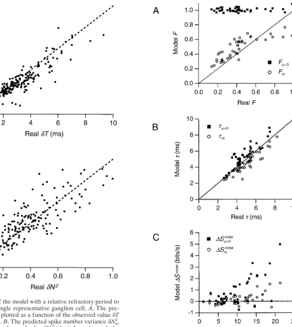
For each cell, the precision of firing events was again measured by the Fano factorFand the temporal jittert. Figure 7A dem-onstrates that the Fano factor Fm predicted from the model
agrees very well with the observed number precisionFfor almost all cells. By contrast, the nonrefractory spike generator always produces a Fano factorFm50near unity, as expected, and in stark
disagreement with the real neurons. Figure 7B shows a similar comparison for the temporal jitter of firing events. Here, one finds that both a relative refractory period and the simple non-refractory model show close agreement with the measured tem-poral jitter, with a slight negative bias using the relative refractory period and a slight positive bias for the nonrefractory model. This Figure 5. Comparison of the model with an absolute refractory period to observed results from a single representative ganglion cell. Six statistics of the spike trains produced by the model are plotted as a function of the absolute refractory periodm. The value of each statistic was averaged over 10 sets of simulated spike trains, and error bars denote61 SD. In each panel, the real value from the neuron is shown by adashed line.A, The average firing rater#m;B, the mean-squared errorEm(solid symbols) and the uncertaintyEm0(open symbols) in the simulated firing rate, with the corresponding
uncertaintyE0in the measured rate (dashed line);C, the Fano factorF
m;D, the temporal jittertm;E, the noise entropy per unit timeSmnoise;F, the
similarity is expected, because the timing precision is derived from the first spike of an event, which is least affected by refractoriness.
The model with a relative refractory period also matched the variety of spiking patterns as measured by the spike train entropy. The total entropy Smtotal predicted using a relative refractory
period was similar to the real valueStotal: the discrepancy was
PSmtotal2 StotalP/Stotal52.9% averaged over the population.
Similarly, the noise entropy was predicted very well with a relative refractory period (Fig. 7C). By contrast, the nonrefractory model produced a large discrepancy between predicted and observed noise entropy, ranging up to 5 bits/sec. In conclusion, a spike generator that incorporates a relative refractory period can very closely reproduce many statistics of real spike trains, whereas a nonrefractory model clearly fails.
The free firing rate
In this model of the spike train, the free firing rate depends only on the external stimulus, whereas the observed firing rate is separated
from the stimulus by an additional, history-dependent nonlinearity. As a result, the free firing rate may be a more fundamental response measure than the observed firing rate. In addition, a refractory period causes the observed rate to saturate whereas the free rate is not so constrained. It is therefore conceivable that the free firing rate can distinguish gradations in the visual stimulus that are lost in the observed rate. Motivated by these ideas, we studied the behavior of the free firing rate of retinal ganglion cells under random flicker stimulation. The free firing rate was estimated using the model with a relative refractory period, which emerged from Figure 6. Comparison of the model with a relative refractory period to
observed results from a single representative ganglion cell.A, The pre-dicted temporal jitterdTmplotted as a function of the observed valuedT for 213 firing events (dots).B, The predicted spike number variancedNm2 plotted as a function of the observed valuedN2(dots). In each panel, the identity relation is shown as adashed line.
Figure 7. Performance of the model with a relative refractory period and the nonrefractory model for a population of 42 ganglion cells from three retinae. In each panel, a statistic derived from simulated spike trains is plotted against the observed value from the same cell; the identity relation is shown as adashed line.A, The Fano factorFm(open circles) and Fm50(solid squares) as a function ofF.B, The temporal jittertm(open circles) andtm50(solid squares) as a function oft.C, The discrepancy in the noise entropyDSmnoise5Smnoise2Snoise(open circles) andDSmnoise50 5 Smnoise50 2Snoise(solid squares) as a function ofSnoise.
the analysis presented above as the most realistic implementation of the refractory properties of a ganglion cell.
Comparison with the observed firing rate
Figure 8 compares the free firing rateqm(t) with the observed
firing rater(t) for a typical firing event. The observed rate rises sharply from zero to its maximum of;300 Hz and then exhibits several peaks (Fig. 8A). The simulated firing rate rm(t) closely
follows these peaks. Figure 8Billustrates the free firing rateqm(t)
on the same scale. At the beginning of a firing event, when refractoriness is negligible,qm(t) is equal tor(t), but it becomes
much larger after several spikes have occurred (Gaumond et al., 1983), ranging up to ;3000 Hz in this case. As a result, the waveform of is even narrower than that ofr(t). Furthermore,qm(t)
is smoother thanr(t), because the ripples introduced by refracto-riness are largely removed. Again, this suggests thatqm(t) is more
closely related to the excitatory input that this neuron receives.
Figure 8C is a scatter plot of the values ofr(t) against values ofqm(t) at the corresponding time throughout the entire
stimu-lus period. Notice that they are roughly equal at low firing rates (q ; 10 Hz), but that r saturates at its maximum of;300 Hz whereasqstill increases. The general shape of this relationship can be understood as a simple consequence of refractoriness: if
q(t) were constant and there were an absolute refractory period of
m, thenrwould reach a steady-state value ofr5q/(11qm). This function provides an upper envelope to the scatter plot in Figure 8C with mchosen as 1.5 msec, close to the absolute refractory period of the real data. Matching the middle of the data cloud is a similar curve usingm53.5 msec, roughly the value that best reproduced the spike train statistics.
The free firing rateqm(t) still varies by more than an order of
magnitude under conditions where the observed rate r(t) has already saturated (Fig. 8C). However, one may ask whether this variation is systematic or is instead introduced by noise in the algorithm that estimates qm(t). After all, the free firing rate is
given by an expression (Eq. 13) with a denominator that is close to zero for large values ofq. To examine this concern, we tested whether these variations in the free firing rate are driven system-atically by the light stimulus.
The light response of the free firing rate
For concreteness, we will assume that the ganglion cell firing rate
r(t) depends on the stimulus intensity with what is called a “Wiener cascade” or “LN model” (Hunter and Korenberg, 1986):
r~t!5f~Z~t!! (20) where
Z~t!5
E
~I~t1t9!2I!L~t9!dt9 (21) Here, the stimulusI(t) is first convolved with a linear filterL(t), and the result Z(t) is transformed at each point in time by a nonlinear functionf(Z). This simple LN model has been used with some success in previous analyses of visual responses (Korenberg et al., 1989; Mancini et al., 1990; Sakai et al., 1995). For a mechanistic picture, one could interpretL(t) as a temporal filter implemented by retinal circuitry. The filtered stimulusZ(t) can be thought of as the effective input to the ganglion cell, and the function f(Z) transforms this input into a firing rate. Of course, the following analysis does not depend on this interpre-tation, nor does it claim that the LN description is a complete account of the light response of the ganglion cells.The parameters of the LN model were deduced from the ganglion cell spike train as follows. First, the linear filterL(t) was obtained by reverse correlation ofr(t) to the Gaussian stimulus
I(t) (Hunter and Korenberg, 1986):
L~t!5*~I~t91*rt~!t29!dtI!9r~t9!dt9 (22) Then, the effective input function Z(t) was computed from Equation 21. Finally, the transformf(Z) was found by plotting the measured firing rate r(t) against the effective input Z(t). The same analysis was applied to derive the LN relationship that links the free firing rateqm(t) to the stimulus. Obviously,
this yielded different parameters, which will be denoted as
Lm(t) andfm(Z).
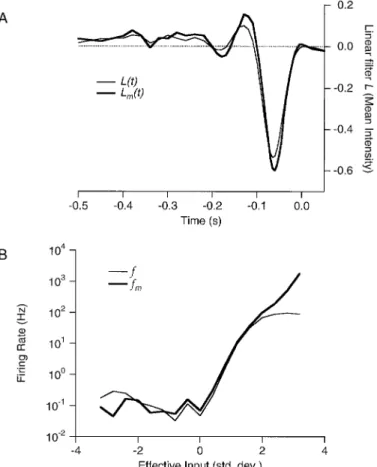
Figure 9Ashows an example of the two linear filters derived Figure 8. A, The observed firing rater(t) (solid line) and the simulated
firing raterm(t) (dashed line) generated by the model with relative refrac-tory period for a single firing event.B, The observed firing rater(t) (thin line) and the free firing rateqm(t) (thick line) for the same firing event. Each curve was computed with 0.25 msec bins, for greater time resolution, and then boxcar-smoothed over nine bins to roughly correspond to the 2 msec bins used elsewhere.C, The observed firing rater(t) computed in 2 msec bins plotted against the corresponding values of the free firing rate qm(t) (dots). Also shown is the steady-state relationr5q/(11qm) for absolute refractory periods of m 5 1.5 msec (dashed line) and m 5
from the observed firing rate and the free rate. The large downward component preceding the action potential indicates that this cell was OFF-type. Both filters have a standard biphasic shape (Sakai et al., 1988; Meister et al., 1994; Smir-nakis et al., 1997), implying a band-pass frequency character-istic, and thus a transient light response. The filter from the free firing rateLm(t) is somewhat stronger thanL(t), especially
in its second peak, and also has slightly shorter latency. This enhancement of the filter can be explained if the largest values ofqfollow more intense stimulus patterns that involve larger excursions from the mean light level. Stronger stimuli also tend to elicit responses faster, consistent with the shorter time-to-peak forLm(t).
Both linear filters were convolved with the stimulus to obtain the effective inputZ(t) andZm(t). Large values of the effective input
occur when the preceding stimulus had a time course similar to the linear filter, whereas small values arise from stimulus patterns that are unrelated. A positive value ofZmarks an intensity variation that matches the sign of the linear filter, for example a brief dimming of the light;70 msec earlier (Fig. 9A), whereas a negative value indicates an intensity variation of the opposite sign.
Figure 9B shows the response function f(Z) obtained by plotting the firing rater(t) against its effective input Z(t). At negative values of Z, the relationship produces a low floor of firing at ;0.1 Hz, which appears unrelated to the effective input. Clearly, this cell does not convey much information about intensity transients of the “wrong” sign. At positive values ofZ, the firing rate rises steeply, and follows an expo-nential dependence over almost three orders of magnitude. Then f(Z) saturates at a firing rate of ;100 Hz. The corre-sponding response function for the free firing rate fm(Z)
follows a similar dependence at lowZ. However, unlikef(Z), it does not saturate at high values of Z, but contin-ues to increase for more than another order of magnitude to ;2000 Hz. Thus, the free firing rate qm(t) can report the
strength of the stimulus over a much wider range thanr(t), up to the strongest intensity fluctuations encountered in these experiments.
DISCUSSION
In summary, we have shown that the light response of a retinal ganglion cell can be captured well by its free firing rateq(t) and its recovery from refractorinessw(t). Both of these functions can be estimated directly from the raw spike trains without free param-eters. This two-component description of the spiking process by
q(t) andw(t) has significant advantages over the traditional anal-ysis of the observed firing rater(t): it accounts correctly for the trial-to-trial variation of the response, the precision of spike timing and spike numbers, and other statistics of the spike train. Furthermore,q(t) continues to vary under conditions in whichr(t) is saturated, and continues to distinguish gradations in the re-sponse of the neuron. Thus,q(t) may prove useful for interpreting the response of any spiking neuron.
Our method relies on determining the recovery functionw(t) directly from the distribution of interspike intervals. The recov-ery function includes both an absolute and a relative refractory period that extend over a short time interval of;5 msec after a spike. These characteristics are consistent with the refractory properties of the ion channels that produce action potentials: sodium channel inactivation leads to an absolute refractory pe-riod and relative refractoriness can result from either shunting or hyperpolarization while the potassium channel remains open (Hille, 1984). Because these ion channels are ubiquitous in spik-ing neurons, one expects the present results to be widely appli-cable also outside the retina.
In fact, the effects of refractoriness on signaling have been studied in cochlear nerve fibers (Gray, 1967; Gaumond et al., 1982, 1983; Johnson and Swami, 1983; Miller and Mark, 1992). Their spike trains reveal absolute and relative refractory periods similar to those of salamander retinal ganglion cells. In cochlear afferents, refractoriness was found to suppress the observed firing rate relative to the free rate by a factor of 2–5 for acoustic clicks and tone burst stimuli (Gaumond et al., 1983; Miller and Mark, 1992). At the onset of spiking episodes, the observed and free firing rates agreed, but the observed rate became most strongly suppressed when it achieved its highest values (Gaumond et al., 1983). In related studies, refractory spike generation helped to explain the power spectrum of spike trains from cochlear affer-ents (Edwards et al., 1993) and from neurons in area MT of the visual cortex (Bair et al., 1994).
Spike trains may also show a long-term dependence on previous activity. Cochlear afferent fibers have, in addition to Figure 9. Analysis of the light response for the observed firing rate
r(t) and the free firing rateqm(t).A, The linear filter relating the light stimulus to the effective input:L(t) for the observed firing rate (thin line) andLm(t) for the free firing rate (thick line).B, The response function relating the effective input to the firing rate: f(Z) for the observed firing rate (thin line) andfm(Zm) for the free firing rate (thick line).f(Z) was obtained by plotting values ofr(t) againstZ(t) every 5 msec, and then binning the range ofZat intervals ofDZ50.4 SD. Thus,f(Z) is the average value ofr(t) over all time points that have an effective input Z(t) between Z 2 DZ/2 and Z 1 DZ/2. The same procedure was followed withqm(t) andZm(t) to obtainfm(Zm).
a refractory period lasting;4 msec, a gradual recovery period extending 20 – 40 msec after an action potential (Gray, 1967; Gaumond et al., 1982). Lowen and Teich (1992) found that successive interspike intervals were not independent, but in-stead showed negative correlations over time intervals up to 100 msec. When firing spontaneously or responding to sus-tained tones, auditory neurons exhibit a spiking variance on long time scales greater than expected from a Poisson process (Teich et al., 1990). Furthermore, salamander ganglion cells show a slowly inactivating outward membrane current (Lukasiewicz and Werblin, 1988) that could contribute to a gradual recovery from spiking. However, when driven by a visual stimulus, these neurons appear strongly locked to the intensity modulations. Spikes are grouped in well defined firing events, and we have found little evidence for correlations extending beyond the typical duration of a firing event. Thus, the present work focused on a recovery function w(t) that implemented only short-term refractoriness.
How should the free firing rate q(t) be interpreted? It is tempting to imagine thatq(t) is directly related to the synaptic currents entering the ganglion cell, whereas the saturation inr(t) results from the refractory properties of its active membrane. If this were the case, then the relationship betweenqandrobserved here (Fig. 8) could also be measured by injecting current into a ganglion cell through an intracellular electrode. Such experi-ments with retinae from salamander (Diamond and Copenhagen, 1995) and turtle (Baylor and Fettiplace, 1979) have reported a rather linear dependence between the injected current and the ganglion cell firing rate. A similar linear relationship has been observed in other spiking neurons (Granit et al., 1966; Lanthorn et al., 1984; Powers et al., 1992). However, the peak firing rates achieved by current injection (50 Hz in salamander) (Diamond and Copenhagen, 1995) were not high enough to sample refrac-toriness. Clearly, it would be rewarding to explore the depen-dence of firing rate on synaptic input over a greater range.
Our analysis of the effects of refractoriness indicates that a longer absolute refractory period serves to improve the response precision of ganglion cells and increase their information rates. Similarly, in the auditory system, realistic refractoriness has been shown to reduce the variance in the response of cochlear afferents to vowel sounds from its value with no refractoriness (Miller and Mark, 1992). These results suggest that a refractory period can improve neural signaling. The refractory period is commonly thought to limit the performance of a neuron, but this view is tied to a preconception about how the cell conveys its signal. If neurons use a “firing rate code,” in which the message lies in the instanta-neous frequency of firing, then refractoriness does reduce the dynamic range of neural output by causing saturation in the firing rate. However, if the message lies in the number of spikes fired during a discrete firing event, then the maximum firing rate is not a limitation, because the cell can simply fire for a longer period of time to produce more spikes. In this case, the refractory period improves the temporal precision of the second and subsequent spikes in an event, leading to a spike count of much higher fidelity than would obtain from a Poisson process. Considering the re-ceiver of such nerve messages, it is plausible that postsynaptic neurons “count” the number of spikes in an event, because the typical firing event duration of;20 msec is within a postsynaptic integration time, whereas the interval between events is much greater.
REFERENCES
Abeles M (1991) Corticonics: neural circuits of the cerebral cortex. Cambridge: Cambridge UP.
Bair W, Koch C, Newsome W, Britten K (1994) Power spectrum analysis of bursting cells in area MT in the behaving monkey. J Neurosci 14:2870–2892.
Baylor DA, Fettiplace R (1979) Synaptic drive and impulse genera-tion in ganglion cells of turtle retina. J Physiol (Lond) 288: 107–127.
Berry MJ, Warland DK, Meister M (1997) The structure and precision of retinal spike trains. Proc Natl Acad Sci USA 94:5411–5416. Bi Q (1989) A closed-form solution for removing the dead time
effects from the poststimulus time histograms. J Acoust Soc Am 85:2504 –2513.
de Ruyter van Steveninck RR, Lewen GD, Strong SP, Koberle R, Bialek W (1997) Reliability and variability in neural spike trains. Science 275:1805–1808.
Diamond JS, Copenhagen DR (1995) The relationship between light-evoked synaptic excitation and spiking behavior of salamander retinal ganglion cells. J Physiol (Lond) 487:711–725.
Edwards BW, Wakefield GH, Powers NL (1993) The spectral shaping of neural discharges by refractory effects. J Acoust Soc Am 93:3353–3364. Ferster D, Spruston N (1995) Cracking the neuronal code. Science
270:756–757.
Gaumond RP, Molnar CE, Kim DO (1982) Stimulus and recovery de-pendence of cat cochlear nerve fiber spike discharge probability. J Neu-rophysiol 48:856–873.
Gaumond RP, Kim DO, Molnar CE (1983) Response of cochlear nerve fibers to brief acoustic stimuli: role of discharge-history effects. J Acoust Soc Am 74:1392–1398.
Granit R, Kernell D, Lamarre Y (1966) Algebraical summation in syn-aptic activation of motoneurones firing within the “primary range” to injected currents. J Physiol (Lond) 187:379–399.
Gray PR (1967) Conditional probability analyses of the spike activity of single neurons. Biophys J 7:759–777.
Hille B (1984) Ionic channels of excitable membranes. Sunderland, MA: Sinauer.
Hodgkin AL, Huxley AF (1952) A quantitative description of membrane current and its application to conduction and excitation in nerve. J Physiol (Lond) 117:500–544.
Hunter IW, Korenberg MJ (1986) The identification of nonlinear bio-logical systems: Wiener and Hammerstein cascade models. Biol Cybern 55:135–144.
Johnson DH, Swami A (1983) The transmission of signals by auditory-nerve fiber discharge patterns. J Acoust Soc Am 74:493–501. Jones K, Tubis A, Burns EM (1985) On the extraction of the
signal-excitation function for a non-Poisson cochlear neural spike train. J Acoust Soc Am 78:90–94.
Korenberg MJ, Sakai HM, Naka K (1989) Dissection of the neuron network in the catfish inner retina. III. Interpretation of spike kernels. J Neurophysiol 61:1110–1120.
Kuffler SW, FitzHugh R, Barlow HB (1957) Maintained activity in the cat’s retina in light and darkness. J Gen Physiol 40: 683–702.
Lanthorn T, Storm J, Andersen P (1984) Current-to-frequency transduction in CA1 hippocampal pyramidal cells: slow prepoten-tials dominate in the primary firing range. Exp Brain Res 53:431– 443.
Lowen SB, Teich MC (1992) Auditory-nerve action potentials form a nonrenewal point process over short as well as long time scales. J Acoust Soc Am 92:803–806.
Lukasiewicz PD, Werblin FS (1988) A slowly inactivating potassium current truncates spike activity in ganglion cells of the tiger salamander retina. J Neurosci 8:4470–4481.
Mancini M, Madden BC, Emerson RC (1990) White noise analysis of temporal properties in simple receptive fields of cat cortex. Biol Cybern 63:209–219.
Meister M (1996) Multineuronal codes in retinal signaling. Proc Natl Acad Sci USA 93:609–614.
Meister M, Pine J, Baylor DA (1994) Multi-neuronal signals from the retina: acquisition and analysis. J Neurosci Methods 51:95–106. Miller MI (1985) Algorithms for removing recovery-related distortion
from auditory-nerve discharge patterns. J Acoust Soc Am 77:1452–1464.
Miller MI, Mark KE (1992) A statistical study of cochlear nerve dis-charge patterns in response to complex speech stimuli. J Acoust Soc Am 92:202–209.
Powers RK, Robinson FR, Konodi MA, Binder MD (1992) Effective synaptic current can be estimated from measurements of neuronal discharge. J Neurophysiol 68:964–968.
Rieke F, Warland D, de Ruyter van Steveninck RR, Bialek W (1997) Spikes: exploring the neural code. Cambridge, MA: MIT.
Sakai HM, Naka K, Korenberg MJ (1988) White-noise analysis in visual neuroscience. Vis Neurosci 1:287–296.
Sakai HM, Wang JL, Naka K (1995) Contrast gain control in the lower vertebrate retinas. J Gen Physiol 105:815–835.
Sejnowski TJ (1995) Pattern recognition-time for a new neural code. Nature 376:21–22.
Shadlen MN, Newsome WT (1994) Noise, neural codes and cortical organization. Curr Opin Neurobiol 4:569–579.
Shannon CE, Weaver W (1963) The mathematical theory of communi-cation, Ed 2. Chicago: University of Illinois.
Singer W, Gray CM (1995) Visual feature integration and the temporal correlation hypothesis. Annu Rev Neurosci 18:555–586.
Smirnakis SM, Berry MJ, Warland DK, Bialek W, Meister M (1997) Retinal processing adapts to image contrast and spatial scale. Nature 386:69–73.
Softky WR (1995) Simple codes versus efficient codes. Curr Opin Neu-robiol 5:239–247.
Stevens CF, Zador A (1995) Neural coding: the enigma of the brain. Curr Biol 5:1370–1371.
Strong SP, Koberle R, de Ruyter van Steveninck RR, Bialek W (1997) Entropy and information in neural spike trains. Phys Rev Lett 80:197–200.
Teich MC, Johnson D, Kumar AR, Turcott RC (1990) Rate fluctuations and fractional power-law noise recorded from cells in the lower audi-tory pathway of the cat. Hear Res 46:41–52.