Modelling and forecasting the volatility of JSE returns: a comparison of competing univariate GARCH models

Modelling and Forecasting the volatility of JSE returns: a comparison of

competing univariate GARCH models

By

Oratile Kgosietsile

A research report in partial fulfillment of the requirements for the degree of Master of Management in Finance and Investment Management

in the

FACULTY OF COMMERCE, LAW AND MANAGEMENT WITS BUSINESS SCHOOL

at the

UNIVERSITY OF THE WITWATERSRA ND

Supervisor: Professor Paul Alagidede

i

DECLARATION

I, Oratile Kgosietsile, hereby declare that the work presented herein is genuine work done originally by me and has not been published or submitted elsewhere for the requirement of a Master in Management of Finance and Investment Management degree at the Wits Business School (WBS). Any literature, data or work done by others and cited within the report has been given due acknowledgement and listed in the reference section. I further declare that I was given authorization by a panel from the research committee of the WBS to carry out the research.

Signed ………

ii

ABSTRACT

The objective of the study was to identify the best approach participants in South African market participants can rely on to model and forecast volatility on the Johannesburg Stock Exchange (JSE). The study models and forecasts volatility (conditional variance) using the GARCH (1, 1), GARCH-M (1, 1), EGARCH (1, 1), GJR-GARCH (1, 1), APGARCH (1, 1), EWMA models and the South African Volatility Index (SAVI). The research relies on data on the FTSE/JSE Top 40 Index returns from 2007 to 2013. It was found that returns on the JSE are categorized by volatility clustering, leptokurtosis and asymmetry. The EGARCH (1, 1) model outperformed all other GARCH models in modeling and forecasting the volatility. When compared to the EWMA and the SAVI, forecasts given by the EGARCH model best described out-of-sample realized volatility. Finally, the study found that the explanatory power of the EGARCH model on out-of-sample realized volatility is enhanced when its forecasts are combined with forecasts from the SAVI.

iii

ACKNOWLEDGEMENTS

I would like to offer my sincerest gratitude to my supervisor Professor Paul Alagidede for all his support, guidance and wisdom shared for the research report. I would also like to thank my mother and father for the emotional strength and continuous motivation throughout the writing process. Lastly, to my family and friends for their never ceasing words of encouragement.

iv

CONTENTS

LIST OF TABLES ... vii

LIST OF FIGURES ... viii

1 INTRODUCTION ... 1

1.1 Objective of the study ... 3

1.2 Significance of the study ... 3

1.3 Organisation of the study ... 4

2 LITERATURE REVIEW ... 5

2.1 Empirical Literature ... 5

2.2 Theoretical framework ... 11

2.2.1 Exponentially Weighted Moving Average (EWMA) ... 11

2.2.2 Autoregressive Conditional Heteroskedastic (ARCH) model ... 12

2.2.3 Generalized Autoregressive Conditional Heteroskedasticity (GARCH) model ... 13

2.2.4 GARCH-in-mean (GARCH-M): ... 14

2.2.5 Exponential GARCH (EGARCH): ... 16

2.2.6 Glosten, Jagannathan and Runkle-GARCH (GJR-GARCH) or Threshold GARCH (TGARCH): ... 17

2.2.7 Asymmetric Power GARCH (APARCH):... 17

2.2.8 South African Volatility Index (SAVI) - Implied Volatility ... 18

2.2.9 Realised Volatility ... 18

3 DATA ANALYSIS ... 20

3.1 Properties of the FTSE/JSE Top 40 ... 20

3.1.1 Descriptive Statistics ... 23

3.1.2 Testing for heteroskedasticity/‘ARCH-effects’ ... 24

3.2 Properties of the SAVI ... 24

3.2.1 Descriptive Statistics ... 25

v

4.1 In-sample model estimates and fit ... 26

4.1.1 Diagnostic checks ... 27

4.2 Forecasting ... 28

4.2.1 Forecast evaluation statistics... 28

4.2.2 Regression based forecast efficiency tests ... 30

5 EMPIRICAL RESULTS ... 32

5.1 GARCH In-sample parameter estimates ... 32

5.1.1 Results of Diagnostic checks ... 34

5.2 GARCH Out-of-sample forecasts ... 35

5.3 In-sample explanatory power: EWMA and SAVI ... 36

5.4 Regression efficiency analysis results ... 37

5.4.1 Out-of-sample forecast ability ... 37

5.4.2 Encompassing Regression for Realised Volatility ... 38

6 CONCLUSION ... 40

6.1 Limitations ... 41

6.2 Recommendations ... 41

7 REFERENCES ... 42

vi

LIST OF ACRONYMS

ADF Augmented Dickey Fuller

APGARCH Asymmetric Power Generalised Autoregressive Conditional Heteroskedasticity

ARCH Autoregressive Conditional Heteroskedasticity

ARCH-LM Autoregressive Conditional Heteroskedasticity – Lagrange Multiplier

CBOE Chicago Board of Options Exchange

EGARCH Exponential Generalised Autoregressive Conditional Heteroskedasticity

EWMA Exponential Weighted Moving Average

GARCH Generalised Autoregressive Conditional Heteroskedasticity

GARCH-M Generalised Autoregressive Conditional Heteroskedasticity in Mean GJR-GARCH Glosten, Jagannathan and Runkle – Generalised Autoregressive

Conditional Heteroskedasticity

HIS Historical Average

JB Jarque-Bera

JSE Johannesburg Stock Exchange

MAE Mean Absolute Error

MAPE Mean Absolute Percentage Error

RMSE Root Mean Square Error

SAFEX South African Futures Exchange

SAVI South African Volatility Index

TGARCH Threshold Generalised Autoregressive Conditional Heteroskedasticity

vii

LIST OF TABLES

Table 1: Unit Root test on Top 40 Index ... 22

Table 2: Descriptive Statistics of the JSE Top 40 Index Returns ... 23

Table 3: Test for ‘ARCH-effects’ in Top 40 Index Returns ... 24

Table 4: Descriptive Statistics of the South African Volatility Index ... 25

Table 5: Estimated GARCH models ... 32

Table 6: Forecast error statistics ... 35

Table 7: Correlation between Realised Volatility and EWMA and SAVI ... 36

Table 8: Regression for Out-of-sample Realised Volatility ... 37

viii

LIST OF FIGURES

Figure 1: Time series plot of the JSE Top 40 Index ... 21

Figure 2: Time series plot of the returns of the JSE Top 40 Index ... 22

Figure 3: Plot of the South African Volatility Index and Top 40 returns ... 25

1

1

INTRODUCTION

Financial markets are well known for their extreme uncertainty and irregularity. Volatility has remained a central concept in finance as there is an important role for volatility modelling and forecasting in all financial markets particularly in investment decisions, security valuation, risk management and monetary policy making (Poon and Granger, 2003). Knowing the volatility of future returns is a useful tool for investors in weighing the risk of holding a financial asset (Bentes and Menezes, 2012). Volatility is also an important variable in the pricing of derivatives securities, whose price is dependent on the predicted future performance of the underlying. Recent history has shown that financial markets have an enormous impact on economies worldwide. Having a good volatility indicator could be a very useful tool to monetary policy decision makers in monitoring the vulnerability of their financial markets and economy (Poon and Granger, 2003). This research will estimate the volatility of the JSE using various measures with the view of finding an appropriate measure that would enable risk managers to properly hedge their positions.

A number of attempts have been made to find the best measure of volatility through a diversified family of models (Poon and Granger, 2003). The success or failure of these volatility measuring models lies in their ability to accurately forecast future volatility. The conventional methods can be classified into two broad categories: volatility derived from time series models based on historical data and volatility implied from option prices.

The most referenced time series models have been the simple historical models and the Generalised Autoregressive Conditional Heteroskedasticity (GARCH) family models. Under the simple historical models, predictions of current equity return volatility are based purely on the behaviour of past standard deviations, these models assume constant variance over time. The GARCH family models assume time-varying variance and models volatility as dependent on lagged conditional variance and lagged squared disturbance. Under the time series models, the GARCH models have been most favored in financial engineering literature. There is a relatively strong body of literature advocating the use of the GARCH family of models to forecast volatility (Engle, 1982; Akgiray, 1989; Brailsford and Faff, 1996; Magnus and Fosu, 2006 ;

2

Samouilhan and Shannon, 2008). These studies have found that the models can adequately model the in-sample equity return volatility. However, there is less evidence that GARCH models provide good out-of-sample forecasts of equity return volatility (Day and Lewis, 1992; Blair et. al. 2000; Tse, 1991; Tse and Tung, 1992). The popularity of the GARCH models is creditable to the models ability to capture the main stylized features that have been observed in financial time series (Fama, 1965; Black, 1976). These are: (i) Time varying volatility – the volatility of stock returns varies with time; (ii) Stock return series have leptokutotic distributions; (iii) Volatility clustering – there is evidence of significant serial correlation between volatility; (iv) Leverage effect – volatility movements tend to be high following negative shocks to the stock market compared to positive shocks to the stock market. These features have been observed in JSE returns (Lesaona et. al., 2011; Niyitegeka and Tewari, 2013; Samoulhan and Shannon, 2008).

The second conventional volatility models, which are also claiming their supremacy over others in measuring volatility in the equity markets, are the option price implied volatility models. One such model is the South African Volatility Index (SAVI) model which was introduced to the JSE price volatility modeling framework by the South African Futures Exchange (SAFEX). The SAVI follows the methodology of the Implied Volatility Index (VIX) which was the first implied volatility index measure introduced to the world of volatility measurement by the Chicago Board of Options Exchange (CBOE) (Tripathy and Gil-Alana, 2010). The VIX still remains the world’s volatility index reference. Research published by the SAFEX describes the methodology for calculating the implied volatility of the FTSE/JSE Top 40 Index from option prices. Proponents of the SAVI highlight its unique ability to gauge and model investor expectations. Since its introduction to the equities trading space in 2007 the SAVI has managed to generally reflect market sentiments hitting its highest levels during times of financial turmoil and when markets recover and investor fear subsides, the SAVI levels tend to drop (Kotzé et. al., 2010; Tripathy and Gil-Alana, 2010).

Despite the importance of conditional volatility, the existing literature has failed to reach a consensus on which model provides the best volatility forecasts. For this reason it is imperative to find the best modeling tool fitting to the South African context specifically. Most studies done on volatility forecasting have been done on developed economies. Thus, from a broader

3

spectrum, there is a need to know around how far one could accurately forecast and to what extent volatility changes can be predicted in the emerging markets (Poon and Granger, 2003). Furthermore, most studies conducted didn’t assess the benefits that the investor would gain from using the best model as opposed to a simpler model. Therefore, in the study we will establish whether the incremental benefit of reliability one receives from using the best model is matched by the cost that goes into generating the model.

1.1

Objective of the study

The motivation of this study is to find the best tool for modeling and forecasting volatility of stock returns on the JSE. In addressing this issue the study will draw its focus on three of the most popular models proposed in the finance and economic literature, the GARCH (p, q), implied volatility and historical volatility. The objective will be to determine the explanatory capabilities and predictive power of univariate GARCH models regarding volatility of stock returns on the JSE and compare these findings to the volatility derived from the implied volatility model (given by the SAVI) and the historical volatility model. The obtained results would allow financial managers to make their optimal financing decisions and build up dedicated hedging strategies. Given these objectives, the research will aim to answer the following questions:

1. What are the stylised features of stock returns on the JSE? Do they behave in such a way that it is possible, through econometric technique, to model and forecast their volatility? 2. How does the univariate GARCH model or any of its extensions perform in modelling

and forecasting volatility?

3. Do the most commonly used methods in financial markets (the historical volatility and the SAVI) accurately model and predict volatility?

4. Which method best models and forecasts volatility of returns on the JSE?

5. How do the easy-to-use models (such as the SAVI) compare to the more complex econometric models (GARCH type models)?

1.2

Significance of the study

This study will benefit all financial market participants on the JSE and South African government monetary policy makers. In particular those that are concerned with portfolio formation, risk management and option pricing will derive utility from it. It will be a useful

4

guide or starting point for them when they are choosing the most appropriate model to use when forecasting volatility for their purposes. On a broader scale, it could also be useful to investors in other emerging markets. Most research into volatility forecasting has been done on developed markets, however emerging markets (particularly African markets) have a fairly different composition to the developed. Investors in other emerging economies with similar financial markets, but who have had no such studies done on their markets could also find the study and its findings useful in their hedging strategies. Understanding the informational content of the SAVI could create a platform for other African economies to introduce volatility indices on their markets which would benefit investors in these markets.

1.3

Organisation of the study

The research paper will begin with a review of the relevant literature on volatility forecasting. This section of the paper will look into significant studies that have been done in the specific research area and bring out any findings that could benefit the particular research. The paper will then present the research methodology used in the analysis of the data, followed by the results found in the analysis. Finally, the paper will conclude on the findings of the analysis, comment on the significance of these findings and point out any gaps in the findings that present grounds for further research.

5

2

LITERATURE REVIEW

This chapter reviews some of the relevant empirical literature and sets the theoretical framework on modelling and forecasting stock return volatility. The first part of the chapter focuses on the empirical literature on modelling and forecasting the volatility of stock returns in both developed and emerging market settings. The second part of the chapter looks at the theoretical literature on the financial econometric models used to model and forecast volatility relevant to this study.

2.1

Empirical Literature

The analysis of financial data, particularly volatility forecasting, is an important task in financial markets and has become an increasingly important topic in finance literature over the last 20 years, especially following the recent financial crisis (Poon and Granger, 2003). A wide variety of models by which volatility forecasting can be achieved have been proposed in financial engineering literature. However, research has produced intriguingly divergent results about which model best performs in forecasting volatility.

The first application of the ARCH model was produced by Engle (1982). The paper studied the variance of UK inflation, it revealed that these models were designed to deal with the assumption of non-stationarity found in real life financial data. The ARCH models treat heteroskedasticity as a variance to be modelled. After this paper, the model quickly gained popularity within the financial engineering space. By the late 1980s authors soon began proposing advancements to the ARCH model in attempts to better model volatility of financial series. The first development was by Bollerslev (1986), which generalised the ARCH model, introducing the GARCH. Studies into time series volatility modeling and forecasting after the Bollerslev (1986) GARCH model have manipulated its raw form to try to model the asymmetric effects observed in financial time series data and long memory in variance. Models such as the GARCH-M, EGARCH, GJR-GARCH, APGJR-GARCH, FIGJR-GARCH, CGJR-GARCH, have been introduced to literature and applied in multiple studies.

The studies into GARCH modelling and forecasting have focused on identifying which GARCH specification best models and forecasts volatility, opposing the performance of symmetric versus asymmetric GARCH models. The symmetric models (GARCH and GARCH-M) are able to capture leptokurtosis (fat tails) and volatility clustering and the asymmetric models (EGARCH,

6

GJR-GARCH, APGARCH, FIGARCH and CGARCH) capture leptokurtosis, volatility clustering, leverage effects and volatility persistence.

Lesaona et. al. (2011) modelled volatility and the financial market risk of JSE returns. The modelling process of the study was conducted in two steps; they firstestimated ARMA (0, 1) models for the mean returns, then fitted the several univariate GARCH models for conditional volatility (the GARCH (1, 1), GARCH-M (1, 1), TGARCH (1, 1) and EGARCH (1, 1) models). The results of the study indicated the existence of ARCH, GARCH and leverage effects in JSE returns over the sample period. Their forecast evaluation indicated that ARMA (0, 1)-GARCH (1, 1) performed best in predicting out-of-sample returns for a period of three months.

Niyitegeka and Tewari (2013) used both symmetric and asymmetric GARCH type models (GARCH (1, 1), EGARCH (1, 1) and GJR-GARCH (1, 1) models) to study volatility of JSE returns. The study also found the presence of ARCH and GARCH effects in JSE returns. However, contrary to Lesaona et. al. (2011) their research failed to identify any leverage effects in return behaviour over the sample.

Alagidede (2011) examined the behaviour of stock returns in six African markets (Egypt, Kenya, Moroccco, Nigeria, South Africa, Tunisia and Zimbabwe). Their research found that the stylised facts typically found in financial time series (volatility clustering, leptokurtosis and asymmetry) are present in African markets stock index returns. The study also found evidence of long memory in all the African markets.

Emenik and Aleke (2012) studied the return volatility of stock returns of the Nigerian Stock Exchange using GARCH (1, 1), EGARCH (1, 1) and GJR-GARCH (1, 1) over the period 2 January 1996 to 30 December 2011. They found evidence of volatility clustering and long memory in the returns. However, the EGARCH and GJR-GARCH produced conflicting results about whether there is asymmetry in the returns.

Abdalla and Winker (2012) studied the performance of different univariate GARCH models in modelling the volatility of major indices on two African Stock Exchanges, the Khartoum Stock Exchange (from Sudan) and the Cairo Alexandria Stock Exchange (from Egypt) over the period 2 January 2006 to 30 November 2010. In the paper, a total of five different univariate GARCH specifications (GARCH, GARCH-M, EGARCH, TGARCH and PGARCH) were considered.

7

They found that returns on the markets are characterised by leptokurtosis, volatility clustering and leverage effects.

Generally research has found that GARCH models have the ability to adequately model the stylised features observed in return behaviour. Brooks (2008) highlights that GARCH models are able to account for the mean-reverting tendency found in volatility series. The study observed that if volatility series are low relative to their historic average they will have a tendency to rise back towards the average, and this phenomenon is modelled by GARCH.

While the use of GARCH models in modelling and forecasting volatility has been relatively well motivated, simple historical volatility models, such as the Random Walk, Historical Mean, Simple Moving Average, Exponential Smoothing and Exponentially Weighted Moving Average methods have remained relevant in financial literature. This is because these models are still a widely used technique for modelling and forecasting volatility on equity markets due to their simplicity.

Akgiray (1989) studied the predictive capabilities of the ARCH/GARCH model in forecasting monthly US stock index volatility compared against forecasts of the Historical Average (HIS) model and an Exponentially Weighted Moving Average (EWMA) model. In this study, Akgiray (1989) found the GARCH model superior to ARCH, EWMA and HIS models for forecasting the volatility. Furthermore, the ARCH/GARCH models capture volatility spikes not captured by the EWMA and HIS models. A visual comparison of actual volatility and volatility predicted by the ARCH and GARCH specifications indicates that these models realistically model the time series behaviour of volatility. These findings display the usefulness and applicability of the ARCH/GARCH framework in forecasting volatility.

Brailsford and Faff (1996) tested the forecasting accuracy of the random walk model, historical mean model, moving average model, exponential smoothing model, exponentially weighted moving average model, a simple regression model, two standard GARCH models and two asymmetric GJR-GARCH models in forecasting volatility of the Australia stock market. In their study, they found that the superiority of a model’s forecasting capabilities is strongly influenced by the choice of error statistic used to assess the accuracy of the model. Thus, they conclude no

8

single model is best but found the GJR-GARCH model slightly superior to the simpler models for predicting Australian monthly stock index volatility.

Magnus and Fosu (2006) model and forecast volatility on the Ghana Stock Exchange using the random walk, GARCH (1, 1), EGARCH (1, 1) and TGARCH (1, 1). The study rejects the random walk hypothesis for GSE returns and finds that the returns are categorised by the main stylised features found in financial data; leptokurtosis, volatility clustering and asymmetric effects.

Tse (1991) and Tse and Tung (1992) used data from the Tokyo and Singapore Stock Exchanges to test the forecasting capabilities of the historical average, EWMA, ARCH and GARCH models. Tse (1991) found that the EWMA method outperformed GARCH and ARCH methods in forecasting the volatility of returns on the Tokyo Stock Exchange. Tse and Tung (1992) applied a similar study to the Singapore Stock Exchange and found the EWMA outperformed the GARCH and historical average methods in forecasting volatility. Tse (1991) found that, there is significant serial dependence of the return series on the Tokyo Stock Exchange. Therefore we would expect the more sophisticated model (the GARCH) that can capture this feature to perform best in forecasting volatility. However, both the studies found that on the contrary the simpler models (EWMA) perform better, and they conclude that this could be due to the fact that the GARCH model has more stringent data requirements (Tse, 1991; Tse and Tung, 1992).

Empirical research has focused on implied volatility given the informational content that is embedded in implied volatility. It is considered an accurate volatility forecast and encompasses all information in other variables. Literature continues to compare the predictability of model based volatility versus implied volatility in a quest to determine which the superior volatility forecaster is. The implied volatility index (VIX) based on S&P 500 returns, from CBOE, has been widely used in both research and practice. Since its introduction to literature, several volatility indices have been introduced around the world.

The implied volatility from index option prices has been widely studied but study results are conflicting. The studies by Day and Lewis (1993), Bluhm and Yu (2000); Samouilhan and Shannon (2008) demonstrated that historical data subsumes important information that is not incorporated into option prices, suggesting that implied volatility has poor performance on

9

volatility forecasting. However, the empirical literature from studies by Blair et. al. (2001), Giot (2005) and Frijns et. al. (2010) documented that the implied volatility from index options can capture most of the relevant information contained in the historical data.

Giot (2005) compared volatility forecasts computed by the VIX and the implied volatility index based on NASDAP returns (VXN), Riskmetrics and GARCH-type models. The study found that the easy-to-use implied volatility indices offer better forecast than the more complex econometric models. Frijns et. al. (2010) applies a methodology similar to Giot (2005) to the Autralian markets. The study also finds that the out-of-sample forecasts from implied volatility perform better than forecasts from Riskmetrics and GARCH type models.

Day and Lewis (1992) studied the out-of-sample forecasting capabilities of the GARCH and EGARCH in forecasting the volatility of the S&P100 index compared with the option implied volatility. The S&P100 index was studied over the period 11 March 1983 to 31 December 1989. They found that in-sample forecasts, implied volatility contains extra information not contained in the GARCH/EGARCH specifications. But the out-of-sample results suggest that predicting volatility is a difficult task. Furthermore, they found that the asymmetry term in the EGARCH model has no additional explanatory power compared with that embodied in the symmetric GARCH model.

Blair et. al. (2000), studied the forecasting power of the S&P 500 (VIX) volatility index, historical volatility and the GJR-GARCH. They found evidence that the incremental information provided by statistical models is insignificant and that the implied volatility index provided the best forecasts. Bluhm and Yu (2000) looked at the performance of the implied volatility index, historical volatility (the Exponentially Weighted Moving Average method) and the EGARCH and GJR-GARCH in forecasting the volatility of the German DAX index. They found that the ranking of the performance of the model varies depending on the forecast horizon and performance measures.

There has only been one study known to the author done on the JSE competing simple historical volatility, GARCH and SAVI volatility forecasts. Samouilhan and Shannon (2008) studied the performance of the ARCH model compared to historical volatility and implied volatility in forecasting the future volatility of the JSE TOP40 index over the period 01/02/2004 to

10

28/09/2006. The paper found that the historical volatility model and the ARCH model are quite poor predictors of volatility. The more complex models such as the GARCH and TARCH perform better. They found the TARCH (2, 2) to be the best in modelling and forecasting volatility, however it is best for one day ahead forecasts as it tends to over predict one week ahead forecasts.

Evidence can be found in empirical literature supporting the superiority of all three models in various financial markets. The conclusion arising from this growing body of research is that forecasting volatility is a very difficult task. Poon and Granger (2003), in a review about forecasting volatility in financial markets, provide some useful insights into comparing different studies on this topic. The authors state that the conclusions of these studies depend strongly on the error statistics used, the sampling schemes (e.g. rolling fixed sample estimation or recursive expanding sample estimation) employed, as well as the period and assets studied.

11

2.2

Theoretical framework

This section looks at some of the various models that have been developed over time to forecast volatility. The section provides basic model descriptions and a theoretical background on some of the financial econometric models that have been proposed to model and forecast volatility specifically those which will be applied in this study. Following the work of Tse (1991), Tse and Tung (1992), Samouilhan and Shannon (2008) and Abdalla and Winker (2012) this study will focus on the following volatility models: (1) The Exponentially Weighted Moving Average (EWMA) model; (2) GARCH (1, 1); (3) GARCH-M (1, 1); (4) EGARCH (1, 1); (5) GJR-GARCH or TGJR-GARCH (1, 1); (6) APGJR-GARCH (1, 1) and (7) The South African Volatility Index. These models are categorised in financial econometric literature as either historical return based volatility models or implied volatility models. Here we outline the theory on these models.

2.2.1 Exponentially Weighted Moving Average (EWMA)

The most prominently volatility forecasting tools used by financial market participants, because of their availability and simplicity, are the EWMA model based volatility and the implied volatility index. In this sub-section we address the EWMA models, the implied volatility index will be covered later in the chapter.

The simplest methods for computing volatility are those whereby predictions are based on past conditional variance. There are a wide variety of models which base current volatility on past conditional variance. These include the Random Walk model where volatility yesterday σt-1 is

used as a forecast for today’s volatility σt (Poon and Granger, 2003). As well as the Historical

Average method, the Exponential Smoothing method and the Exponentially Weighted Moving Average method (Poon and Granger, 2003). Due to its wide usage within literature, the study focuses on the EWMA model from this class of volatility models.

Under the EWMA, the forecast of volatility is a function of the immediate past forecast and the immediate past observed volatility each assigned a certain weight (Brailsford and Faff, 1996; Brooks, 2008). The EWMA can be calculated as follows:

12

is the smoothing parameter, and must be 0 ≤ ≤ 1. If is zero, then the EWMA model becomes a random walk model, i.e. volatility is a function of its immediate past observed volatility. As approaches one, then more weight is given to the prior period forecast which itself is heavily influenced by its immediate past forecast and so on (Brailsford and Faff, 1996; Brooks, 2008).

The main advantage of the EWMA model is that it is easy to use and relatively it has produced good results in literature (Tse, 1991; Tse and Tung, 1992). Its disadvantage is that after sudden price movements the model has the tendency to significantly overestimate volatility.

2.2.2 Autoregressive Conditional Heteroskedastic (ARCH) model

Conventional time series and econometric models rely on the premise of Ordinary Least Squares which assumes that the variance of the disturbance term is constant. However, it has been observed that many economic and financial time series display periods of unusually high volatility followed by periods of relative tranquillity. In such situations, the assumption of a constant variance is no longer appropriate.

The ARCH model was first invented in the early 1980s by Robert Engle, he introduced this model because he saw the need to have a model that recognizes the dynamic volatilities of returns (the fact that variance is not constant but conditional on time). Thus, instead of using short or long sample standard deviations, the ARCH model proposed taking weighted averages of past squared forecast errors, a type of weighted variance (Engle, 2004). ARCH class models make use of the sample standard deviations but formulate conditional variance of returns as a function of previous information via maximum likelihood procedure (Omwukwe et al., 2011). An ARCH (q) model can be specified as follows.

In the Mean equation of the ARCH model

= +

where = return on asset at time t, = average return, and = residual returns defined as:

=

13 The conditional variance (volatility) is denoted as:

= +

with constraints > 0 and ≥ 0(for all i = 1,…,q) to ensure is positive.

The main disadvantage of the ARCH model is that it restricts the model for the conditional variance to follow a pure AR process and hence it may require more parameters to adequately represent the conditional variance process in comparison with other more generalized models. As a result in modelling ARCH there might be a need for a large lag q, which may consequently result in a model with a large number of parameters, violating the principle of parsimony. This violation potentially presents difficulties when using the ARCH model to sufficiently describe the data. Another disadvantage in the ARCH model is that in an ARCH (1) model, next period's variance only depends on last period’s squared residual. This is a potential issue such as in the case of a crisis; a crisis that caused a large residual would not have the sort of persistence that we observe after actual crises. These issues led to the introduction of the GARCH model.

2.2.3 Generalized Autoregressive Conditional Heteroskedasticity (GARCH) model

After the ARCH model, a generalization of it was then later introduced by Bollerslev (1986), the Generalized Autoregressive Conditional Heteroskedasticity (GARCH), which generalizes the purely autoregressive ARCH model to an autoregressive moving average model. Under the GARCH the conditional variance depends on the squared residuals and on its past values, the generalisation allows it to be seen as a prudent model that avoids over fitting. The GARCH model is the most widely used model today (Brooks, 2008). In the classical GARCH models, the conditional variance is expressed as a linear function of the squared past values of the series. This particular specification is able to capture the main stylized facts characterizing financial series (fat tails and volatility clustering).

The GARCH (p, q) can be specified as follows:

14 = + _{+ "} # $ # _#

where the current conditional variance () is parameterised to depend upon q lags of the squared error and p lags of the conditional variance (Brooks, 2008). With constraints > 0 and

≥ 0(for all i = 1,…,q), "_# ≥ 0 (for all i = 1,…,p) and α + β < 1. The latter constraint on α + β ensures that the unconditional variance of ε_& is constant, even though its conditional variance evolves over time. The unconditional variance is given by: Var (ε_&) = '(

(')*+) when α + β < 1. For α + β ≥ 1, the unconditional variance of ε_& is not defined, and this means the model is non-stationary in variance. A model whereby α + β = 1 is one that is unit root in variance, it is also known as an ‘Integrated GARCH’ model or IGARCH. It is important to note that this stationarity condition (α + β < 1) is to be satisfied as there is no theoretical justification for models whose summation of the lagged residual term and the lagged conditional variance is more than one. “For stationary GARCH models, conditional variance forecasts converge upon the long-term average value of the variance as the prediction horizon increases. For IGARCH processes, this convergence will not happen, while for α + β > 1, the conditional variance forecast will tend to infinity as the forecast horizon increases.” (Brooks, 2008) The GARCH (p, q) reduces to an ARCH (q) model if q=0.

2.2.4 GARCH-in-mean (GARCH-M):

In financial markets, the return of a security may be influenced by its volatility. The GARCH-M, by Engle et. al. (1987), is still a symmetric model of volatility, however it differs to the classical GARCH model in that it introduces conditional volatility term to the Mean equation to account for the fact that the return of a security may depend on its volatility. The GARCH-M (1, 1) can be written as:

Mean equation: = + +

_{= +}

+ "

r& represents the return of a security, and μ and λ are constant parameters to be estimated. The

15

risk premium over the sample period. The GARCH-M specification relaxes this assumption by allowing volatility feedback effect to become operational (Brooks, 2002). The parameter λ is called the risk premium parameter. The parameter λ represents the conditional volatility term that is introduced in the GARCH mean equation to account for the fact that the return of a security may depend on its volatility. If λ is positive and statistically significant, it implies that the return is positively related to its volatility and an increase in risk given by an increase in conditional variance leads to an increase in mean return, and vice versa. The implication of a statistically positive relationship would mean that an investor on the South African equity market is being compensated for assuming greater risk. If however, such a relationship is negative this could imply that during times of great volatility or uncertainty investors react to a factor other than the standard deviation of stocks from their historical mean, possibly skewness.

ASYMMETRIC GARCH MODELS:

As stated earlier, the classical GARCH model and the GARCH-M model in their modelling are able to capture two stylised facts of financial data: leptokurtosis (fat tails) and volatility clustering. A major disadvantage of the GARCH and GARCH-M is that they are symmetric models and thus unable to account the asymmetric feature of financial data. This asymmetric feature is commonly known as the leverage effects. The leverage effect observed in financial data has been shown in various empirical studies; it is the tendency for bad news to have a more pronounced effect on the volatility of asset prices than do good news. In other words, the volatility increase due to a price decrease is generally stronger than that resulting from a price increase of the same magnitude.

Consequently, after the GARCH, variants of it were then introduced to literature each one aiming to account for this phenomenon and other stylized features (for example the long memory phenomenon) in financial returns that the former did not (Brooks, 2008). These include the Exponential GARCH (EGARCH), GJR-GARCH or Threshold GARCH (TGARCH), Asymmetric Power GARCH (APARCH) and Integrated of Fractionally Integrated (FIGARCH)

16

these models are called the asymmetric GARCH models. Asymmetric GARCH models are designed to capture leverage effects. Specification of each of these models is as follows1:

2.2.5 Exponential GARCH (EGARCH):

The EGARCH was proposed by Nelson (1991). The first advantage of the EGARCH is that, its specification ensures that, even if the parameters are negative, the conditional variance is always positive since it is expressed as a function of logarithm (Omwukwe et al., 2011). The second advantage is that, asymmetries (leverage effects) are allowed for since if the relationship between the volatility and returns is negative, γ, will be negative. The EGARCH (1,1):

ln _{= + 1}||

3− 4

2

67 − 8₃+ "ln

A problem with symmetric GARCH models is that it is necessary to ensure that all of the estimated coefficients are positive, we did so in the GARCH(p,q) specification above by stating the constraints > 0 and ≥ 0(for all i = 1,…,q), "_# ≥ 0 (for all i = 1,…,p). Nelson (1991) proposes the exponential GARCH (EGARCH) model that does not require non-negativity constraints. Since it is the log of conditional variance (ln) regardless of the parameters being negative the conditional variance will remain positive hence the need to artificially impose non-negativity constraints does not arise. In modelling lnwe see that the leverage effect is exponential versus quadratic and validating that conditional variance will be non-negative. In addition, the EGARCH model allows for the asymmetric effect of news or shocks on the conditional volatility. 8 is the asymmetry coefficient. If 8 < 0 and statistically significant, then negative shocks imply a higher next period conditional variance than positive shocks of the same magnitude, this is where the model accounts for asymmetric impacts (Brooks, 2008; Emenik and Aleke, 2012).

1

This study focuses solely on using univariate GARCH models to forecast volatility. Therefore, we specify the extensions of the GARCH model that follow in their univariate form.

17

2.2.6 Glosten, Jagannathan and Runkle-GARCH (GJR-GARCH) or Threshold GARCH (TGARCH):

The GJR model (named for Glosten, Jagannathan and Runkle, 1993) extends the classical GARCH model by adding an additional term to account for possible asymmetries. The GJR-GARCH(1,1):

= + + 8 + "

where = 91 :;

_{< 0}

0 :; ≥ 0

The TGARCH model developed by Zakoian (1994), takes an approach similar to that taken in the GJR-GARCH model. The TGARCH model introduces a threshold effect (in the form of a dummy variable) into the volatility to account for leverage effects.

= + + 8= + "

Where dummy variable == 9 1 :;

_{< 0, ?@= ABCD}

0 :; ≥ 0, EFF= ABCD

∅is the asymmetry component and is the asymmetry coefficient. The presence of leverage effects will mean that the coefficient of asymmetry will be positive and significant (i.e. > 0). The reasoning behind this is similar to that of the EGARCH model, where negative news will have a greater impact on volatility than good news of the same magnitude.

2.2.7 Asymmetric Power GARCH (APARCH):

Ding et. al. (1993) introduced the parameters δ and ς into the GARCH family. The parameter δ is an exponent that may be estimated as an additional parameter, this enhances the flexibility of the model. The parameter ς is added to capture asymmetry.

H = + (|| − Ϛ)H+ "H

The main advantage of this model is that it is flexible, very general and contains the standard GARCH, the TGARCH, and the Log-GARCH. The model is a standard GARCH (1, 1) by Bollerslev (1996) when δ = 2 and Ϛ = 0, a TGARCH (1, 1) by Zakoian (1994) when δ = 2 and a Log-GARCH by Geweke (1986) when δ → 0.

18

2.2.8 South African Volatility Index (SAVI) - Implied Volatility

The implied volatility index is a model based on current option price data, and for this reason is commonly referred to as the ‘fear gauge’. The most referenced equity market ‘fear gauge’ in the world is the VIX, a Chicago Board of Options Exchange (CBOE) product. A similar index has recently been developed for the South African equity markets, the SAVI, launched in 2007. The SAVI is based on the Top 40 Index and it is computed on a daily basis using the three month at-the-money volatility (Kotzé et. al., 2010). Thus, the SAVI represents a daily measure of Top 40 at-the-money implied volatility over the following three months (Samouilhan and Shannon, 2008).

The SAFEX follows a similar methodology to the CBOE in order to calculate the SAVI. The basis for the calculating the SAVI is the methodology adapted in Whaley (1993), but because of the limited liquidity of the SAFEX, instead of the regular one-month as the rolling fixed maturity period, the SAVI uses an extended three month period.

In this study implied volatility is defined as:

(L MN) = SAVI2

where SAVI is the volatility index published by the SAFEX.

The disadvantage of the SAVI is that it is not suitable for all products (only for that which are an underlying for an actively traded option) and it may be unreliable sometimes because it is dependent on the irrational expectations of investors. Its advantage however is that it is easy-to-use and it has strong theoretical motivation.

2.2.9 Realised Volatility

The model-free estimator of observed volatility (conditional variance) of returns that has been proposed in literature is realised volatility (Day and Lewis, 1993; Blair et. al., 2000; Bluhm and Yu, 2000; Giot, 2005; Frijns et. al., 2010). In this study an estimator of the market’s volatility is needed to estimate EWMA volatility as well as to assess the informational content of the various volatility forecasts, the details of the methodology will be outlined later in Chapter 4. Realised volatility is defined as the sum of squared daily returns

19

OM = PQ

20

3

DATA ANALYSIS

This research applies the FTSE/JSE Top 40 index across the various volatility models to study the volatility of JSE returns. The Top 40 index is a market capitalization weighted index of the 40 largest companies in the FTSE/JSE All-Share Index ranked by full market values. Over the sample period the Top 40 Index represented an average of about 80% of the market value of the All-Share Index, as well as the most actively traded shares. The Top 40 index therefore serves as a good proxy of the South African share market.

The study focuses on the period 01/02/2007 to 31/12/2013. This is a particularly interesting period over which to study stock price volatility on the JSE because of the developments this stock exchange undertook in 2007 that influenced volatility. On 2 April 2007, the JSE adapted the London Stock Exchange’s new equity system called TradeElect. The TradeElect system has increased the performance of the market because of the increased liquidity and significant reduction in trading costs (SAIFM, 2008). The increase in liquidity and reduction in trading costs could have had an impact on volatility of the prices of securities traded on the JSE due to the fact that trading in shares and other securities is now a cheap and viable option.

Merton (1980) observed that the accuracy of volatility estimates using past volatility increases as the sampling frequency over the observation period increases. Therefore, the study applies daily index levels to the volatility models. To the author’s knowledge, daily observed closing levels are the highest frequency publicly available on the Top 40 Index. The SAFEX publishes data on the SAVI, which are obtained from the McGregor-BFA database. Data obtained on the daily closing levels of the Top 40 Index on the JSE during this period is applied to the GARCH models and historical volatility modelling. This data is obtained from Bloomberg database.

3.1

Properties of the FTSE/JSE Top 40

In Figure 1 below is a plot of the Top 40 Index close prices over the period of study. From a visual inspection, a distinct major event stands out, the sharp upturn around the beginning of 2007 followed a dramatic fall in the index during 2008 around the time of the global financial crisis. The global financial crisis resulted in a fall in key export markets, lower commodity prices and a slowdown in capital flows to developing countries all negatively impacted the South African economy during the financial crisis which spilled over into the performance of shares on

21

the JSE (Balchin, 2009). After the 2008 downfall we see the Top 40 price picking up again in 2009 and a general upward trend until the end of 2013 with minor recoveries and slumps.

The trend observed in the price series resembles a random walk process. The price series only crosses its mean value of 27688.74 occasionally and generally tends to moves away from this mean value over the period. This means that the price series is non-stationary.

Figure 1: Time series plot of the JSE Top 40 Index

The price series can be transformed via a logarithm into a return series in order to make it stationary. The Top 40 index daily price levels are transformed into returns by this simple operation:

= TA UVV

W

where Pt and Pt−1 are current and previous stock prices for t = 1, 2, · · · , ∞.

15,000 20,000 25,000 30,000 35,000 40,000 45,000 2007 2008 2009 2010 2011 2012 2013 TOP40LEVELS

22

Figure 2: Time series plot of the returns of the JSE Top 40 Index

Figure 2 above is a plot of the transformed price series, the Top 40 Index return series, which resembles a white noise process. The series visibly has no upward or downward trending behaviour and frequently crosses its mean value of 0.0126%. This means the return series could now be stationary. These findings can be verified using a formal test for stationarity known as the Augmented-Dickey Fuller (ADF) test. Under the ADF test, we test for the null hypothesis that the series has a unit root. The results are presented in Table 1 below.

Table 1: Unit Root test on Top 40 Index

Levels First Difference (Log-returns) Top 40 Index -0.3453 -41.1652

Critical values of ADF test at 1%, 5% and 10% are -3.4337, -2.8629 and -2.5676 respectively

The ADF test statistic for the series in level terms is statistically insignificant, meaning the Top 40 price series is non-stationary. The ADF test statistic for the series in first difference terms is highly significant; therefore we conclude that the Top 40 Index return series is stationary.

Finally in a preliminary analysis of the plotted return series in Figure 2, the series displays a tendency for volatility to occur in clusters. Volatility clustering means that in the series we see periods where there are relatively higher and lower positive movements (around 2008, 2010 and 2011) and periods of relatively lower positive and negative movements. This is a phenomenon commonly observed in financial time series.

-.12 -.08 -.04 .00 .04 .08 2007 2008 2009 2010 2011 2012 2013 TOP40RETURNS

23 3.1.1 Descriptive Statistics

Before applying formal econometric methodology, several descriptive statistical tests are performed on the Top 40 index returns which include reporting on the mean, skewness, kurtosis and the Jacque-Bera (JB) test for normality. The purpose of this is to check the distributional properties of the return series before applying formal econometric tests.

Table 2: Descriptive Statistics of the JSE Top 40 Index Returns

Observations Mean Median Maximum Minimum Std. Dev. Skewness Kurtosis JB statistic 1803 0.000320 0.001090 0.077069 -0.079594 0.014471 -0.082217 6.631026 992.5057

(0.0000) Notes: p-value of JB test statistic is reported in parentheses

The average return for the return series was approximately 0.032%. The returns had a maximum value of 7.7069% and minimum -7.9594%, giving the series a range of 15.6663% over the period studied.

Skewness measures the extent to which a distribution is not symmetric about its mean value (Gujarati and Porter, 2009). A normal distribution is symmetric about its mean and has a skewness of zero. The skewness of the return series was -0.0822. This means the series was negatively skewed and majority of the returns were less than the mean return. Kurtosis measures how fat the tails of the distribution are (Gujarati and Porter, 2009). A normal distribution has a kurtosis of three. The excess kurtosis for the return series was 6.631. A kurtosis greater than three means that the TOP40 Index returns are peaked around their mean value, these returns are termed leptokurtosis, and this is the distribution more likely to characterise a financial time series (Brooks, 2008).

Finally we examine the Jarque-Bera (JB) test statistic for normality. Under the JB test we test for the null hypothesis that the returns are normally distributed. The JB test is statistically significant at the 1% level (p-value < 0.01), leading us to reject the null that the returns are normally distributed and conclude that the Top 40 Index returns are not normally distributed. These findings tie in with the negative skewness and leptokurtosis found in the series.

The findings in our preliminary analysis of the return series; volatility clustering, leptokurtosis and non-normality, suggest that the variance of the daily returns is not constant over time. These

24

findings led to the next hypothesis test conducted in the study, a formal test for the time-varying feature of the variance of this series.

3.1.2 Testing for heteroskedasticity/‘ARCH-effects’

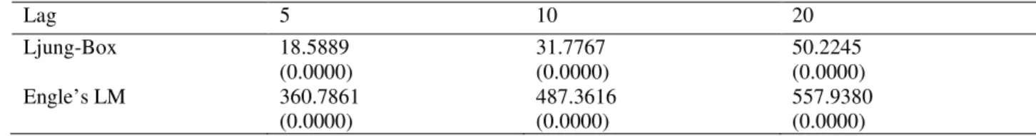
The test for heteroskedasticity will be done using the Box statistic suggested by Ljung-Box (1978) and Engle’s LM test by Engle (1982). The Ljung-Ljung-Box statistic, tests for the null hypothesis that “all m autocorrelation coefficients are zero”, which occurs when ARCH effects are present. Under the Engle’s LM test, we are testing for autocorrelation in the squared residuals. We test for the joint null hypothesis that “all q lags of the squared residuals have coefficient values that are not significantly different from zero”, which is the case when no ARCH effects exist (Brooks, 2008).

Following the procedure outlined by Brooks (2008) for running the ARCH test, the first step taken is to estimate an ARMA (1, 1) model for the Top 40 Index Returns via Least Squares estimation. Then run the Heteroskedasticity ARCH test on the squared residuals in Eviews. As a base, we start at 5 lags of the squared residuals as suggested by Brooks (2008), but also test at a further 10 and 20 lag lengths. The Ljung-Box test is run on the return series, also through Eviews. The results are presented in Table 3 below, both the Ljung-Box and Engle’s LM statistics are highly significant at all lag lengths, indicating that there is a presence of heteroskedasticity/ ‘ARCH effects’ in the Top 40 Index returns.

Table 3: Test for ‘ARCH-effects’ in Top 40 Index Returns

Lag 5 10 20 Ljung-Box 18.5889 (0.0000) 31.7767 (0.0000) 50.2245 (0.0000) Engle’s LM 360.7861 (0.0000) 487.3616 (0.0000) 557.9380 (0.0000) Notes: p-values are reported in parentheses

3.2

Properties of the SAVI

Figure 3 below plots the SAVI and Top 40 returns over the period of study. One major event stands out in Figure 3, we see a sharp increase in volatility around 2008 when the Top 40 index experienced a sharp decline in the wake of the global financial crisis. Before and after the major

25

downfall, the Top 40 Index only experienced minor recoveries and slumps which are well represented by increases in the SAVI.

Figure 3: Plot of the South African Volatility Index and Top 40 returns

3.2.1 Descriptive Statistics

The descriptive statistics of the SAVI are examined to understand how it explains the behaviour of volatility over the period studied. Table 4, presents the descriptive statistics of the SAVI. The average level of the volatility was approximately 24.5039%. The volatility of the Top 40 Index according to the SAVI, ranged from a maximum value of 57.9700% and minimum 13.5100% over the period studied. The high maximum value can be related to the sharp downfall seen towards the end of 2008 in Figure 1, and the volatility cluster observed in Figure 2 and 3 also around that time where the returns reach their highest and lowest values within that year. The SAVI is non-normally distributed with positive skewness, leptokurtosis and a highly statistically significant JB test statistic.

Table 4: Descriptive Statistics of the South African Volatility Index

Observations Mean Median Maximum Minimum Std. Dev. Skewness Kurtosis JB statistic 1804 0.245039 0.229700 0.579700 0.135100 0.073425 1.521391 6.159166 1446.121

(0.0000) Notes: p-value of JB test statistic is reported in parentheses

-.1 .0 .1 .2 .3 .4 .5 .6 2007 2008 2009 2010 2011 2012 2013 SAVINDEX RETURN

26

4

METHODOLOGY

This chapter outlines the methodology which will be employed in the study to address the research issues. The first subsection outlines the methods for estimating the in-sample parameters of the various models. The second subsection describes the forecasting approach that will be taken in the study and the technique that will be used to evaluate the univariate GARCH model volatility forecasts (the forecast evaluation statistics). The final subsection will outline the regression based efficiency test methodology from Giot (2005) and Frijn et. al. (2010) which will be used to evaluate the volatility forecasts across all models (GARCH, EWMA and SAVI).

4.1

In-sample model estimates and fit

The EWMA model is constructed based on the previous period realised volatility, where realised volatility is proxied by the squared excess returns. Historical models therefore do not need to be estimated as they are constructed. Similarly, volatility given by the SAVI does not have parameters to be estimated, in this study we will judge the in-sample ‘fit’ or explanatory power of these models based on their correlation with squared excess returns as done by Samoulhan and Shannon (2008). The GARCH models however have parameters that need to be estimated.

Estimation of GARCH models

In the presence of heteroskedasticity, Ordinary Least Squares estimation is no longer appropriate. In order to estimate GARCH models we employ the Maximum Likelihood method for parameter estimation. This method simply chooses a set of parameters that have most likely generated observed data, using an iterative computer algorithm (Brooks, 2008). The variance equations for the GARCH models to be estimated in the study and their mean equations have been specified in chapter 3. For illustrative purposes we will focus on the GARCH (1, 1) in outlining the Maximum Likelihood procedure, as the same methodology applies across the various GARCH specifications.

The most important step in the estimation of this model is to form a log-likelihood function which we maximise with respect to the parameters. A search using Marquardt’s numerical iterative algorithum, which will be run through Eviews in this study, then generates the

27

parameter values that maximise the log-likelihood function. Assuming follow a normal distribution, the log-likelihood function to maximise can be written as:

TFEX = −12 TFE(26) −12 TFE() −12 (⁄ )

Research has shown however that the normality assumption is not always satisfactory and there are instances when non-normality conditions are present in the distribution of . In such instances, alternative standard error distributions such as the Student-t distribution by Bollerslev (1987), the Generalised Error Distribution (GED) by Nelson (1991) or the standard Cauchy distribution may be considered. For purposes of this study we shall assume the normalised residuals () follow a student-t distribution to account for fat tails, as observed in our data analysis (Alagidede, 2011). For the student-t distribution the log-likelihood function to be maximised then becomes:

TFEX = −1_{2 TFE Z}6([ − 2)\([ 2_{\(([ + 1) 2⁄ )}⁄ )] −1_{2 TFE() −}([ + 1)

2 TFE Z1 + (

₎

_{([ − 2)]}

given \(∙) is the gamma function and the degree of freedom v > 2 is the shape parameter which controls for the fat tails. As [ → ∞ the student-t distribution converges to the normal distribution.

4.1.1 Diagnostic checks

After estimating the GARCH models, diagnostic tests will be performed on the residuals of the estimated models to establish whether the model has been correctly specified and guard against spurious inferences. Diagnostic tests check for non-linearity in the residuals. The common principle behind these tests is that once a model has been generated non-linear structure is removed from data and the remaining structure should be due to an unknown linear data generating process (Alagidede, 2011). This study will examine the residuals for non-linearity using with three different tests; the Ljung-Box-Q, the ARCH-LM and a BDS test on residuals as done by Magnus and Fosu (2006).

The Ljung-Box and ARCH-LM tests have already been used in the study, under section 3.1.1., to check for the presence of autocorrelation and heteroskedasticity for the raw series. Under our

28

diagnostic checks, we will be computing the same tests for the standardized residuals of each of the GARCH model (Magnus and Fosu, 2006). The nonparametic BDS test by Brock et. al.

(1996) examines the non-linearity of residuals. The null hypothesis of BDS diagnosis test is that the data are pure white noise (completely random).

4.2

Forecasting

We forecast the one-month-ahead (30-days-ahead) volatility. The one-month-ahead volatility will be found by static (a series of rolling single-step-ahead) forecasts using Eviews. The sample data contains the first 1804 daily observations. The models will be estimated over the in-sample data. The estimated parameters are used to obtain one-month-ahead volatility forecasts.

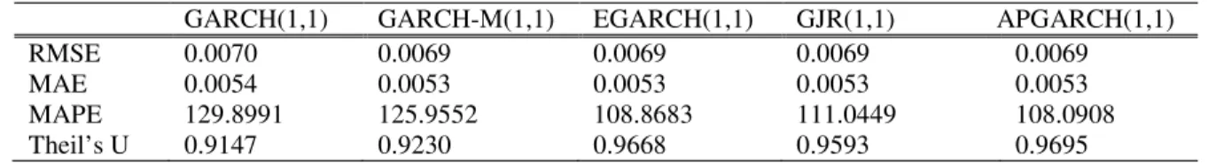
4.2.1 Forecast evaluation statistics

The forecasting performance of the models will be evaluated based on their statistical loss functions. Some of the most commonly used forecast accuracy measures in literature which will be used in this study are the Root Mean Square Error (RMSE), Mean Absolute Error (MAE), Mean Absolute Percentage Error (MAPE) and Theil’s U-statistic (Brailsford and Faff, 1996; Brooks, 2008). RMSE = ` S(S) )a ( ₋ ) S S) MAE = S(S) )a b ₋ b S S) MAPE = cc S(S) )a b( ₋ )/b S S) Theil’s U-statistic = ef Ughigjhi g_hi W S S) ef Ughigjkhi g_hi W S S) l

where T represents the number of total observations (both in-sample and out-of-sample) and m is the first out-of-sample forecast observation. Therefore, the model is estimated by the observations from 1 to m− 1 and observations from m to T are used for the out-of-sample

29

forecasting. and denote the actual and the estimated conditional variance at time t,

respectively. _n is obtained from a benchmark model (in this study the benchmark model will be the random walk model).

“RMSE and MAE measure how far the forecast is from the actual data, thus the forecast with the smallest RMSE and MAE is probably the most accurate forecast (Brooks, 2008).

RMSE provides a quadratic loss function (Brooks, 2008). The advantage of the RMSE is that it is most sensitive to large errors of the four criterions, due to the squaring of the errors. Therefore, it is most advantageous where there are large estimate errors that could lead to serious problems. However, the RMSE can bottleneck if there if are large errors that cannot lead to serious problems. MAE measures the average absolute forecast error (Brooks, 2008). The advantage of the MAE is that it penalizes large errors less than the RMSE because it does not square the errors.

Although the function form of RMSE and MAE are simple, they are inconstant to scalar transformations and symmetric this implies that they are not very realistic in some cases (Brooks, 2008).

MAPE essentially tells us how well the forecast is able to account for variability in the actual data (Brooks, 2008). It measures the percentage error, its value is restricted between zero and one hundred percent. Therefore, the forecast with a MAPE closest to 100 is probably the most accurate. The advantage of MAPE is that it can be used to compare the performance of the estimated models and random walk model. For a random walk in the log level, the criterion MAPE is equivalent to one. Therefore, an estimate model the MAPE which is smaller than 100 is considered to be a better one than random walk model. However, the disadvantage of this error is that it is not reliable if the series take on the absolute value which is smaller than one.

The Theil’s U-statistic compares the forecast performance of the model to the performance of a benchmark model. A U-statistic = 1 implies that the model under consideration has the same accuracy/inaccuracy as the benchmark model. If U-statistic < 1, then the estimated model is considered to be better than the benchmark model. If U-statistic equals one, it suggests that the estimated model has the same accuracy as the benchmark model. The advantage of this error is that comparing Theil’s U-statistic is constant to scalar transformation but it is symmetric.”

30 4.2.2 Regression based forecast efficiency tests

Once the best performing univariate GARCH model has been identified using the forecast error statistics, its out-of-sample predictive power will be evaluated against the EWMA and SAVI using simple OLS regressions, a methodology similar to those adapted in Day and Lewis (1992), Giot (2005) and Frijns et. al. (2010). The efficiency, informational content and unbiasedness of the volatility forecasts will be assessed by studying their relationship with out-of-sample RV.

Out-of-sample forecast ability:

We will examine the out-of-sample forecast capability of each model by regressing realised volatility on a constant and the forecast from each model:

(1)OM = + " o + *

(2)OM = + "L MNo + *

(3)OM = + "q Orso + *

where _o , L MN_o and q Ors_o is the forecast given by the various models. Under this method we essentially test the joint unbiased null hypothesis that = 0 and "= 1, in which case the forecast of that particular model accurately forecasts actual volatility. The good volatility forecast would also present a high adj-R2.

Out-of-sample informational content:

To examine the out-of-sample forecast informational content of the models, we will run the following encompassing regression:

(1)OM = + "q Orso + "L MNo + *

(2)OM = + "q Orso + "t o + *

(3)OM = + "L MNo + "t o + *

31

From the above encompassing regressions we determine whether the forecast performance of one approach is superior to the other or whether when models are used together they can complement each other and perform better in forecasting. From studying the results of the encompassing regression, we will be able to understand the how the models perform against each other as well as whether combining different models can increase their individual explanatory power.

32

5

EMPIRICAL RESULTS

This chapter presents the results of the study. The results have been presented in two stages, the first stage was to evaluate the modelling and forecasting performance of the various GARCH models amongst themselves and the second stage took the best performing GARCH model and evaluated it against the EWMA and SAVI.

5.1

GARCH In-sample parameter estimates

The estimates for the univariate GARCH models are presented in Table 5 below. The models estimated via the maximum likelihood procedure assuming the normalised residuals () follow a student-t distribution.

Table 5: Estimated GARCH models

GARCH(1,1) GARCH-M(1,1) EGARCH(1,1) GJR(1,1) APGARCH(1,1)

Estimates of Mean Equations

µ 0.0008*** (3.1796) 0.0006* (1.6528) 0.0003 (1.1912) 0.0003 (1.4021) 0.0003 (1.0338) λ 1.8026 (0.8090)

Estimates for Conditional Variance

ω 1.90E-06*** (2.638) 1.91E-06*** (2.6471) -0.1719*** (-5.4296) 1.26E-06*** (3.318) 0.0001 (1.0047) α1 0.0962*** (6.2724) 0.0963*** (6.2702) 0.0915*** (4.8079) -0.0155 (-1.3177) 0.0601** (2.1505) β1 0.8961*** (56.0942) 0.8959*** (55.9140) 0.9888*** (347.3162) 0.9375*** (88.4743) 0.9381*** (86.8872) γ -0.1198*** (-8.6677) 0.1390*** (7.5346) 1.0000 (1.4175) δ 1.0619*** (5.3241) d LL 5415.118 5415.426 5445.201 5439.852 5446.079 α1 + β1 0.9923 0.9922 1.0803 0.922 0.9982 Information Criteria AIC -6.0012 -6.0005 -6.0335 -6.0276 -6.0334 SBIC -5.9860 -5.9822 -6.0153 -6.0093 -6.0120 HQIC -5.9956 -5.9937 -6.0267 -6.0208 -6.0255 Diagnostic Results of Residuals

Q-stat 9.0871 [0.524] 8.9643 [0.535] 12.149 [0.275] 10.142 [0.428] 10.93