Are
Multiple
Cross-Correlation Identities better than
just
Two
? Improving the Estimate of Time
Differences-of-Arrivals from Blind Audio Signals
Danilo Greco
?,†?Universit`a degli Studi di Genova (DITEN)
Via All’Opera Pia, 11a 16145 Genova, Italy danilo.greco@{edu.unige.it, iit.it}
Jacopo Cavazza
†,‡†Pattern Analysis and Computer Vision (PAVIS)
Istituto Italiano di Tecnologia (IIT) Via Enrico Melen, 83
16152 Genova, Italy [email protected]
Alessio Del Bue
†,‡‡Visual Geometry and Modelling (VGM)
Istituto Italiano di Tecnologia (IIT) Via Enrico Melen, 83
16152 Genova, Italy [email protected]
Abstract—Given an unknown audio source, the estimation of time differences-of-arrivals (TDOAs) can be efficiently and robustly solved using blind channel identification and exploiting the cross-correlation identity (CCI). Prior “blind” works have improved the estimate of TDOAs by means of different algorith-mic solutions and optimization strategies, while always sticking to the case N = 2 microphones. But what if we can obtain a direct improvement in performance byjustincreasingN? In this paper we try to investigate this direction, showing that, despite the arguable simplicity, this is capable of (sharply) improving upon state-of-the-art blind channel identification methods based on CCI, without modifying the computational pipeline. Inspired by our results, we seek to warm up the community and the practitioners by paving the way (with two concrete, yet preliminary, examples) towards joint approaches in which advances in the optimization are combined with an increased number of microphones, in order to achieve further improvements.
Index Terms—Acoustic Impulse Response, Blind Channel Identification, Incremental and Ensembling Approaches, TDOA Estimation
I. INTRODUCTION
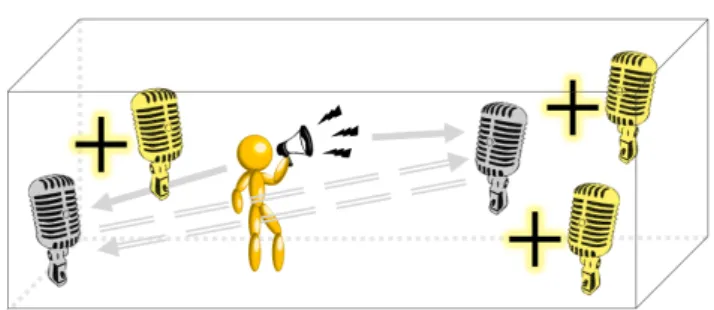
Sound source localisation applications can be tackled by inferring the time-difference-of-arrivals (TDOAs) between a sound-emitting source and a set of microphones. Among the referred applications, one can surely list room-aware sound reproduction [1], room geometry’s estimation [2]–[6], speech enhancement [7], [21] and de-reverberation [8]–[10]. Despite a broad spectrum of prior works estimate TDOAs from an known audio source [22]–[24], even when the signal emitted from the acoustic source isunknown, TDOAs can be inferred by comparing the signals received at two (or more) spatially separated microphones [10], [11], [14], [17], [18] using the notion of cross-corrlation identity (CCI) - see Fig. 1. This is the key theoretical tool, not only, to make the ordering of microphones irrelevant during the acquisition stage, but also to solve the problem asblindchannel identification [10], [11], [14], [17], [18], robustly and reliably inferring TDOAs from an unknown audio source (see Sec. II).
Fig. 1. We are given an unknown sound-emitting source, where in the actual applicative scenario that we encompass, we have no prior knowledge about the sound source and can be therefore arbitrary. We are interesting in (robustly) inferring TDOAs in an (unknown as well) environment given a pool of microphones, using the the following principle. Given the pair of grey microphone, the audio that each of them acquires from the source (solid arrow) must “agree” with the other. That is, if any of the two mic could “hear” the other, the registered signal has to be the very same (dashed arrows). This is calledcross-correlation identityand it was empirically studied in the case N= 2, only. In this paper we answer to what happens then ifN >2? Can we improve in robustness and/or accuracy in the estimate, for instance, by adding the yellow microphones?
However, when dealing with natural environments, such “mutual agreement” between microphones can be tampered by a variety of audio ambiguities such as ambient noise. Fur-thermore, each observed signal may contain multiple distorted or delayed replicas of the emitting source due to reflections or generic boundary effects related to the (closed) environment. Thus, robustly estimating TDOAs is surely a challenging prob-lem and CCI-based approaches cast it as single-input/multi-output blind channel identification [10], [11], [14], [17], [18]. Such methods promotes robustness in the estimate from the methodological standpoint: using either energy-based regular-ization [11], sparsity [10], [17], [18] or positivity constraints [17], while also pre-conditioning the solution space [10].
In this paper, we posit that there is a much easier practical strategy to ensure robustness while inferring TDOAs: the possibility of exploiting a larger pool of microphones. In fact, it
is surprising to observe that, in prior state-of-the-art methods based on CCI, experimental evidences are provided for the case N = 2 microphones only [10], [11], [14], [17], [18]. Despite such a number is the bare minimum to solve the problem, it remains elusive whether N > 2 can, by itself, boost the estimate of TDOAs in accuracy/robustness, without requiring any changes in the computational pipeline. In fact, since all methods [10], [11], [14], [17], [18] cantheoretically accommodate forN >2, why not test them in such a regime? The purpose of this work is to answer this question and back up the investigation of state-of-the-art methods based on CCI [10], [11], [14], [17], [18] in handling the case N >2. Our goal is to understand whether an increase in the number of microphones will translate into an improved TDOAs estimate. Our contributions. Among all state-of-the-art methods based on CCI [10], [11], [14], [17], [18], we consider the most effective one: IL1C [10]. Despite, in fact, recent advances were essentially devoted in estimating TDOAs given a known audio source in how to exploit the TDOAs [22]–[24], the problem of achieving the very same task while being blindly unaware of which audio source was deployed can be still efficiently and effectively solved using methods such as [10], [11], [14], [17], [18] out of which IL1C [10] is the best in terms of robustness and efficacy. IL1C infers TDOAs by solving a stack of convex problems through a weighted sparsity promoting (`1) constraint, leveraging the non-negativity of the Acoustic
Impulse Response (AIR), from which TDOAs are easily estimated using peak finding [10]. To guarantee robustness while inferring TDOAs, in addition to sparsity, IL1C [10] takes advantage of a pre-conditioning mechanism to better initialize the AIRs using a data-driven initialization.
We setup a broad experimental validation, measuring the performance of IL1C on a variety of audio signals, going well beyond the experimental evidences provided in [10]. That is, on the one side, we test the effectiveness of this method on many more audio signals: synthetic (pink and white) noise and a list of natural audio sources (two different plastic rustles – obtained from either scraping a bag or compacting a bottle before thrashing, adult male voice, dog barking, stapler and hand-clapping). On the other side, differently to [10], we do not only consider the case N = 2, but we also consider a bigger number of microphones N = 3,4,5,10 motivated by encompassing the scenario of multiple microphones.
As our experimental evidences show, we stably register improvements in either the robustness (towards outliers) or the accuracy in retrieving the peaks of the AIRs. We evaluate on that by exploiting two well known performance metrics as in prior work [10], [11], [14], [17], [18], and, although there are (sound-specific) cases in which one of the two indicators show a damaged performance, still the other one shows im-provements. In fact, we can demonstrate that, across the wide number of different audio sources that we consider, the general trend is that, while averaging the absolute improvement across different choices for N = 3,4,5 or 6 over the baseline case
N = 2, we score positive signed improvements (see Table III) which seems not to be effected on whether the source is
emitting synthetic or natural sounds. At the same time, we register a very positive trend if we are enriched by an oracle knowledge of the optimal number of microphones that have to be arranged before the acquisition stage. In such a case, we always register positive improvements over the baseline
N = 2, which are, in the worst case, by+3%, while achieving more than+28% as well.
Inspired by our evidences, in Section V, we attempt to warm up future research directions towards optimization approaches which explicitly account for the case N > 2. Although proposing a new paradigm which falls inside this new family of methods is out of scope for us, we still deem interesting to inform practitioners about the effect of two straightforward modifications of IL1C [10], using either an incremental pre-conditioning or an ensemble strategy - see Section V. Re-gardless of the scores results (in which the ensemble strategy is better than the incremental pre-conditioning, while also improving the baseline IL1C method [10]), we deem our effort to be effective in stimulating the research towards methods which explicitly account for the case N > 2 when dealing with an unknown audio source.
II. PROBLEMSTATEMENT& RELATEDWORK
Let us formalize the problem of inferring TDOAs, so that we can easily refer to prior related works. Let us consider a given enviroment (e.g., a room) of unknown geometry in which an audio source emits together with N microphones: the task is to reconstruct TDOAs.
Lethnrepresent the AIR (Acoustic Impulse Response) from a fixed audio source and then-th microphone,n= 1, . . . , N. The signal hn is sampled into a fixed number of temporal bins hn(k). The signal yn(k) received at microphone n can be written as the discrete convolution between the transmitted signalx(k)and then-th AIR:
yn(k) =hn(k)∗x(k) +νn(k), n= 1, . . . , N (1)
where νn(k)is an additive noise term. The ultimate goal of the problem is leveraging the measurementsyn(k)to recover the AIRshn(k)without knowing the transmitted signalx(k). Cross-correlation identity. When multiple microphones are recording the same audio source, the acquisition should be independent of the order of the microphones according to the following constraint:
hm(k) ∗ hn(k) ∗ x(k) =hn(k) ∗ hm(k) ∗ x(k), (2) for every pairs of microphones m and n. In turn, using eq. (1), we rewrite eq. (2) ashm(k) ∗ yn(k) =hn(k) ∗ ym(k). Hence, by using the well-known fact that the convolutional operator∗ is linear, we obtain
Ynhm=Ymhn, m, n= 1, . . . , N (3)
wherehn is the column vector which stacks the AIRshn(k) by columns, while Yn is the diagonal-constant matrix with first row and column given by [yn(k − K + 1), yn(k −
2), . . . , yn(k),0, . . . ,0]>respectively, withKandLbeing the signal length and channel length.
In order to solve for (3), a number of prior approaches have took advantage of regularization [10], [11]. For instance, Tong et al.[11] have framed the problem of TDOAs estimation as the following regularized Least Squares fitting
min h1,...,hN X m6=n kYnhm−Ymhnk22 s.t. X i khik22= 1, (4)
to ensure robustness by means of regularization. Clearly, adding a regularization term is fundamental to avoid the optimization to converging towards the trivial solutionhn= 0 for every n = 1, . . . , N. Remarkably, the real problem is choosing a proper regularization term.
In fact, when using`2regularization - as in eq. (4), the solu-tion can be computed in closed-form by means of eigenvalue decomposition [11]. Unfortunately,L2 regularization neglects
some crucial physical properties of the expected solution -such as non-negativity [13], [14].
Additionally, requiring P
ikhik
2
2 = 1as in (4) makes the
AIRs to be co-prime [15] and constraint each of them to have a fixed norm - each of such requirements are likely to introduce numerical instabilities and artifacts during the optimization process. As a remedy for this, sparsity priors have been successfully applied to a broad spectrum of prior work in TDOAs estimation [1]–[6] [15], while also encompassing speech enhancement [16] and de-revereberation [8]. Therefore, as to impose sparsity in the reconstructed hn, replacing the
L2 regularization in eq. (3) with a L1 counterpart [10], [17],
[18] seems an appealing solution. Precisely, in [18] aL1-norm
penalty was added to eq. (4), yielding
min h1,..,hN X m6=n kYnhm−Ymhnk22s.t. (P ikhik 2 2= 1, P ikhik1< ε. . (5)
Unfortunately, a quadratic optimization subject to mixed quadratic and linear constraints do not preserve the convexity of (4). Hence, the method as in (5) is prone to local solutions.
To cope with this issue, we can relax eq. (3) into
min h1,..,hN X m6=n kYnhm−Ymhnk22s.t. ( |h1(a)|= 1, P ikhik1< ε. , (6)
where the fixed index a is an anchor constraint [17] which makes the optimization in eq. (6) convex and more robust towards spectrum holes ofx(k)if compared to eq. (4).
However, the anchor constraints|h1(a)|= 1together with P
ikhik1 < ε penalizes all the peaks intensities but one,
often leading to peak cancellations in noisy conditions. The approach of [17] has been modified in [14] adding an ancillary non-negativity constraint on the AIRs
min h1,..,hN X m6=n kYnhm−Ymhnk22s.t. |h1(a)|= 1, P ikhik1< ε h1, ..,hN ≥0. , (7)
where, for eachn,hn ≥0meanshn(k)≥0for eachk. Non-negativity yields increased robustness against noise by further
regularizing the problem [19], [20], but it is arguably limited in addressing the limitations of the anchor constraints.
To directly tackle the latter problem, Crocco et al. [10] replaced the anchor constrained |h1(a)|= 1by means of the
introduction of a slack variables p1, . . . ,pN such that
min h1,..,hN X m6=n kYnhm−Ymhnk22s.t. pn>hn = 1, P ikhik1< ε h1, ..,hN ≥0. (8)
In this way, all the components of the AIRs are equally taken into account without privileging the a-th of the h1. At the
same time, differently from eqs. (5), (6), the constraints as in eq. (8) are differentiable, since h1, ..,hN ≥ 0 implies
P
ikhik1 = Pi
P
ahi(a). The optimization problem as in eq. (8) is convex with respect to hn while fixing the slack variables pn and vice-versa. Inspired by this consideration, Crocco et al. [10] proposed an alternated iterative scheme in which, pn are firstly initialised as the AIRs computed using Tong et al. method’s [11], while cycling between: 1) optimizing forh1, ..,hN in (8) givenp1, ..,pN and 2) use the newly computed AIRs to updatepn for everyn. As discussed in [10], although the proposed initialization introduces a distortion in the amplitude of the AIRs, then the iterative procedure is able to compensate. More crucially, initializing pn at the first iteration by using [14] makes the slack variable sparse. Therefore, the first two constraints as in eq. (8) make the computed AIRs sparse again. Such property is preserved during optimization because of the updating scheme in which slack variables at a given iteration are selected as the solution of eq. (8) as in the prior iteration.
A sharp limitation of prior blind methods. None of the prior methods [10], [11], [14], [17], [18] was generalized to the case
N > 2. Despite N = 2 has the appealing formal property
of achieving minimality among the number of microphones necessary to solve the optimization problem, still it remains elusive from a practical standpoint whether allocating for a bigger number N of microphones can effectively boost the estimate of TDOAs. And, in the likely event of this case effectively happening, are we improving upon robustness towards outliers or in accuracy as well? The scope of the present work is to answer this question.
III. MULTIPLECROSS-CORRELATIONIDENTITIES
In this Section, we evaluate the effect of increasing the number of microphones when tackling the problem of infer-ring TDOAs by means of well established notion of cross-correlation identity (CCI) [10], [11], [14], [17], [18]. In details, we focus on IL1C [10], the best out of such class of approaches: we optimize equation (8) for the case of N= 2,3,4,5,10. By doing so, we are capable of starting from the minimal setup from which the problem can be solved (N = 2): note that this is the experimental playground analysed in prior works [10], [11], [14], [17], [18]. Differently, for the sake of inspecting whether a higher number of microphones can provide an improvement in the estimate of TDOAs, we also
consider the casesN= 3,4,5up to theN = 10microphones. This range of variability inN is, in our opinion, a good trade-off between having a sufficiently large number of acquisition devices, while still framing a scenario which can be still useful from the applicative standpoint.
Let us briefly introduce the types of source signals consid-ered in this study, as well as the reproducibility and imple-mentation details about our evaluation protocol and the error metrics to check on performance. The results of our analysis are reported in Tables I and II, while showing relative and absolute improvements in Table III. An extended discussion on our findings is reported in Section IV.
The different types of source signals we considered. We considered two types of synthetic audio signals white noise and pink noise, which differ among each others in the con-sidered frequencies of their spectrum (all vs. only wide ones, respectively). We also encompass a broad list of natural sounds as audio source: plastic rustle no. 1 (bag),plastic rustle no. 2 (bottle),adult male voice,dog barking,staplerand hand-clapping, all of them characterized by a narrow frequency spectrum.
Evaluation. We run experiments by considering any of the source audio signals described in the prior paragraph located in the same environment analyzed in [10]. We model the Acoustic Impulse Response (AIR) for each microphones as seven different peaks, corresponding to one direct path source-microphones, together with six (first-order) reflections. In details, we applied the simulating image method as in [16], using a reflection coefficient of0.8. We also introduce another degree of variability, by considering different Noise-to-Signal ratios (s). This is done by injecting additive Gaussian white noise on the output microphones according to the following specs:0 dB, 6 dB , 14 dB, 20 dB and 40 dB. This induces a signal-to-noise ratio s = 10−dB/20 from the following
inverse relationship dB = 20 log10(1/s). When running the optimization (8) of IL1C [10], we take advantage of the official code directly shared by authors, while following the same pre-processing and evaluation techniques as in the referred prior work. In addition, as done (8), we perform model selection by doing cross-validation on the threshold ε which controls the sparsity-promoting constraint.
Error metrics.Once the AIRs have been computed through (8), we apply the peak finding method of [10] and we evaluate performance by means of two standard error metrics: the Average Peak Position Mismatch (APPM) and the Average
Percentage of Unmatched Peaks (APUP) [15]. To ensure
statistical robustness towards the random generation of reflec-tions using [16], we performed Z = 50 random repetitions of the experiments using Monte-Carlo simulation [10]. A ground truth peak is considered to be unmatched if the closest estimated number is more than a fixed number of samples aways from it (we follow [10] in setting this value equal to 20). In formulæ, we compute APPM and APUP in the following
manner APPM= 1 Z Z X i=1 ¯ Pi X p=1 |τp,i−τep,i| ¯ Pi (9) APUP= 1 Z Z X i=1 K−P¯i K (10)
where P¯i is the number of ground truth peaks for which a matching has been found among the estimated ones: such value is indexed over the Monte-Carlo simulations i =
1, . . . , Z. For every i and given an arbitrary p = 1, . . . , Pi
τp,i, in eq. (9), τp,i and eτp,i are the p-th ground truth peak location and its corresponding estimate, respectively. In eq. (10), K denotes is the number of ground truth peaks of the source signal.
By means of such metrics, we can decouple the effect of the outliers (quantified by APUP) from the overall peak position
accuracy (expressed by APPM), ultimately better evaluating
on the robustness with which TDOAs are estimated. IV. THE PROPOSEDTEST-CASE:ADISCUSSION
Performance differences across variable s values. An in-creasing value fors will make the acquired signal noisier, so that, in Tables I and II the case s = 0.01 is (much) easier with respect to s = 1. This visually translates into errors (and histogram bars) which increase when moving from left to right in the referred error tables. A sharp increase of errors is registerd on white noise(synthetic) and bag plastic ruslte,
adult male voice and dog barking (natural). Differently, on either pink noise (synthetic) or stapler, hand-clapping (natural), we can see that already the case s= 0.01is challenging per se. We posit that a reason for that is the highly oscillatory natura of those sounds that, if compared to other cases, make them less influeced by the additive Gaussian noise (since they behave as if they were intrinsically noisy)
Differences between synthetic and natural sound-emitting sources.Let us comment on whether the usage of a synthetic versus a natural source emitting sound can have an impact on the final performance. According to the experimental results reported in Tables I and II, while also inspecting the signed absolute/relative improvements of Table III, we can get that there seems not to be a sharp difference in performance between these two categories. In fact, we did not register any drop/raise when swapping from white/pink noise to the other sounds considered in this work. We deem this a valuable property of the cross-correlation identity (CCI) which can naturally accommodate for a variety of applicative scenarios where the audio source is unknown.
Does adding microphones improves upon performance?
We are intended in enriching this discussion with a detailed analysis on the ultimate question that our work is trying to respond. We believe that the findings of Tables I and II are plain: the honest answer to the aforementioned question we are intended to respond is neither positive nor negative, in
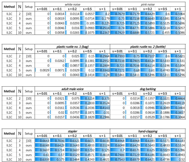
TABLE I
AVERAGEPEAKPOSITIONMISMATCH(APPM))METRICS FORIL1C [10]WHENN= 2,3,4,5,10. SYNTHETIC SOURCE NOISE ARE DENOTED IN
ITALIC,WHILE BOLD ITALIC REFERS TO THE NATURAL SOURCE SIGNAL CONSIDERED IN THIS STUDY. FOR EACH SOURCE SIGNAL CONSIDERED,WE PROVIDE AN HISTOGRAM VISUALIZATION TO BETTER PERCEIVE THE VARIABILITY OF THE ERROR METRICS:THE RANGE OF VARIABILITY OF EACH DATA
BAR IS NORMALIZED WITHIN EACH DIFFERENT SOURCE SIGNAL. ABETTER PERFORMANCE CORRESPONDS TO A LOWER(APPM))VALUE OR,
EQUIVALENTLY,TO A LOWER BAR. THE VALUEsQUANTIFIES THE IMPACT OF THE ADDITIVEGAUSSIAN NOISE ON THE REGISTERED SIGNAL:WE SPAN THE CASEs= 0.01(EASIER)TOs= 1(HARDER),WHILE TRANSITIONING ON THE INTERMEDIATE CASESs= 0.1,0.2ANDs= 0.5.
general. In fact, there is a quite number of cases in which the addition of microphones is not clearly beneficial, on the contrary damaging performance: for the sake of brevity, let us report the worst cases for the two metrics. That is, the cases s = 1, N = 10 and hand-clapping for APPM
(-1.4031 absolute improvement) ands= 1,N = 4 andadult male voiceforAPUP (-0.0393 absolute improvement). These
are definitely failure cases and, specifically, hand-clapping,
s = 1 for APPM is clearly not positive since the trend is
that performance drops whileN increases. Albeit these cases are surely negative, let us observe that there are actually no cases where concurrently the two metrics deteriorate. In fact, in the worst cases, only one of the two is damaged: we either loose in effectiveness on how we handle outliers or in how accurately we retrieve the peaks. But, globally the case
N >2 is never inferior to the baseline N = 2 with respect
to both metrics concurrently.
At the same time, let us observe that these failure cases are
limited since, in the majority of the (remaining) cases, the performance is either stable (therefore adding microphones is not detrimental) or better (and thus addding microphones actually help). The fact that performance is stable when varying the number of microphones is true for the (less noisy) casess= 0.01,pink noise, forAPPM; s= 0.01, adult male voice, for both APPM andAPUP; s = 0.01, pink noise, for
APUP;s= 0.01dog barking, for APPM.
Finally, let us concentrate on the ideal cases, where the performance improves when N raises. This happens for (the more challenging) cases such as s = 1 dog barking, for APPM;s= 0.5adult male voice, forAPPM;s= 0.1,stapler,
for APPM ands= 0.5,adult male voice, for APUP,s= 0.1
ands= 0.2,plastic rustle no. 2 (bottle)for APUP; s= 0.2, dog barking forAPUP.
Given the alternate nature of the results, when switching from one error metric to another and while varying differents
TABLE II
AVERAGEPERCENTAGE OFUNMATCHEDPEAKS(APUP)METRICS FORIL1C [10]WHENN= 2,3,4,5,10. SYNTHETIC SOURCE NOISE ARE DENOTED
IN ITALIC,WHILE BOLD ITALIC REFERS TO THE NATURAL SOURCE SIGNAL CONSIDERED IN THIS STUDY. FOR EACH SOURCE SIGNAL CONSIDERED,WE PROVIDE AN HISTOGRAM VISUALIZATION TO BETTER PERCEIVE THE VARIABILITY OF THE ERROR METRICS:THE RANGE OF VARIABILITY OF EACH DATA
BAR IS NORMALIZED WITHIN EACH DIFFERENT SOURCE SIGNAL. ABETTER PERFORMANCE CORRESPONDS TO A LOWER(APUP))VALUE OR,
EQUIVALENTLY,TO A LOWER BAR. THE VALUEsQUANTIFIES THE IMPACT OF THE ADDITIVEGAUSSIAN NOISE ON THE REGISTERED SIGNAL:WE SPAN THE CASEs= 0.01(EASIER)TOs= 1(HARDER),WHILE TRANSITIONING ON THE INTERMEDIATE CASESs= 0.1,0.2ANDs= 0.5.
of our findings in the next part of our discussion.
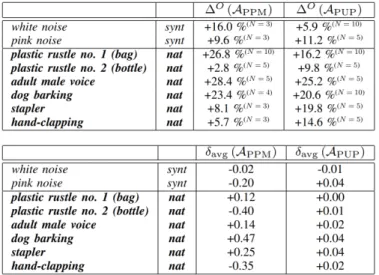
A summary of the improvements. In Table III (bottom), we report the average absolute signed improvementδavgover
the two error metrics APPM andAPUP: the overall majority
of the cases show a superiority of the case N > 2 with respect to the baseline case N = 2 of IL1C [10]. This is exemplified from the fact that the signed improvement is positive (δavg > 0) for 5 out of 8 different audio signals,
in terms ofAPPM, and 7 times out of 8, in terms ofAPUP.
Despite of their sign, the absolute value of such improvements is controlled (it never exceeds 0.5). This trend is explained from the fact that, there are high fluctuations, sometimes, between different configurations inside the case N > 2 for an unknown audio source.
To better investigate this trend, we also consider the signed relative improvements ∆O of the error metrics A
PPM and
APUP (Table III, top). In this case, we allow for an oracle
selection of the best number N of the microphone configu-ration so that we can understand what is the “upper” bound on the improvement that we can expect to register. The results are extremely encouraging: wealwayshave significant positive improvements. In the worst cases (plastic rustle no. 2 (bottle), APPM), we get a +2.8% while, in the most favorable case
(adult male voice,APPM), the relative improvement sharply
raises, reaching +28.4%.
V. FUTUREPERSPECTIVES
In shed of the results of our test-case (Table III), we deem now reasonable for practitioners to start investigating the regime N > 2 (unknown source) with computational methods which take advantage of this scenario in explicit terms. Although this actual effort is beyond the scope of the present submission, we are nevertheless interested in warming up the research in this direction by considering what are, to our opinion, the easiest modification that can be applied to the
TABLE III
SIGNED IMPROVEMENTS FOR THE METRICSAPPMANDAPUPWHEN
COMPARINGN >2WITH THE BASELINEN= 2USING THE STATE-OF-THE-ART METHOD[10].Top:WE PROVIDE THE PERCENTAGE
RELATIVE IMPROVEMENTS∆OUSING THE ORACLE SELECTION FOR
MICROPHONE NUMBER’S CONFIGURATION(REPORTED AS A SUPERSCRIPT).Bottom: WE PROVIDE THE MEAN ABSOLUTE IMPROVEMENTδavgACROSSallCASESN= 3,4,5,10WITH RESPECT TO
THE BASELINEN= 2.Top and Bottom: WE REPORT THE AFOREMENTIONED STATISTICS FOR THE MORE CHALLENGING
NOISE-TO-SIGNAL RATIOs= 1.
state-of-the-art method IL1C [10]. In the rest of the present Section, we will present two computational variants of IL1C which are either based on anincremental pre-codintioningor anensemble mechanism.
Incremental pre-conditioning. Given the core contribution of pre-conditioning the solution that IL1C introduced, we can think about anincrementalpreconditioning in which we grad-ually introduce one microphone, intertwining this operation with a fine-tuning of the AIRs. That is, we start from a pair of microphones and we optimize for it. Then, we use the solutions of IL1C for that pair to pre-condition the solution when solving for a third microphones: we the update also the AIRs for the first two microphones. The procedure iterates until theN-th microphones is added (so that theN−1AIRs of the other microphones are fine-tuned, at least one time). Let us formalize the prior argument in the following pseudocode. 1. Sample two random microphonesm1,m2.
2. Optimize eq. (8), using the standardpre-conditioning [10], thus obtaining the AIRs form1 m2.
3. Add a third microphonem3: optimize eq. (8) again but now
changing the preconditioning. The AIRs of m1 andm2 will
be the ones obtained at the previous stage, while the AIR of
m3 will be initialized using the standard approach [10].
4. Update the AIRs for all solved microphones.
5. Keep adding microphones, following the same procedure, until allN ones are covered
Results & Discussion. We did not register any substantial improvement using this sequential addition, to the point that even the caseN = 2is superior in performance. For the sake
of brevity, let us report a glance of the scored results, providing a peculiar case which is aligned with the general trend which we do not report for the sake of brevity. For white noise, the results of incremental strategy describe above are 0.0036 (s= 0.01), 0.0357 (s= 0.1), 0.09 (s= 0.2), 0.1536 (s= 0.5) and 0.2343 (s= 1) forAPUP and 0.2658 (s= 0.01), 0.5866
(s = 0.1), 1.0023 (s = 0.2), 1.7345 (s = 0.2) and 2.2391 (s = 1) for APPM – all error values refer to the case with
N = 4, while averaging overZ= 50random extraction of the sequence with which microphones are incrementally added. We explain this lack of improvement with the fact that, despite adding microphones in a single solution maybe beneficial, their sequential addition can be detrimental since, albeit on the one side the case N >2is providing more cues than the baselineN = 2, the sequential addition of microphone would lead to “over-fitting” the AIRs of some of the microphones, ultimately damaging the final performance.
Ensemble mechanism. Let us observe that the inference stage of IL1C [10] is based on peaks finding, a method which is known to suffer when spurious peaks are present. To accommodate for that, let us take advantage of the following approach. We can split the caseN >2into severalN = 2 sub-problems, by pairing microphones into couples. We therefore create a number of playgrounds with 2 microphones only (unknown source) - so that we match the operative conditions on which IL1C [10] was originally tested. We therefore create some redundancy in the estimate of the AIRs: this is because one microphone can belong to several pairings at the same time, so there will be multiple candidate solutions for the same AIRs - two candidates, referring to two different microphones, from each artificial pairing. We solve for this redundancy by averaging out all different candidates referring to the same microphone. We deem this approach to be arguably simple, perhaps rough, but still effective in handling a well known computational issue which damages peak findings algorithm. In fact, the presence of spurious (noisy) peaks surely affect the estimate of TDOAs. We attempt to mitigate this problem by exploiting the well known smoothing and regularizing properties of averaging as our ensemble mechanism.
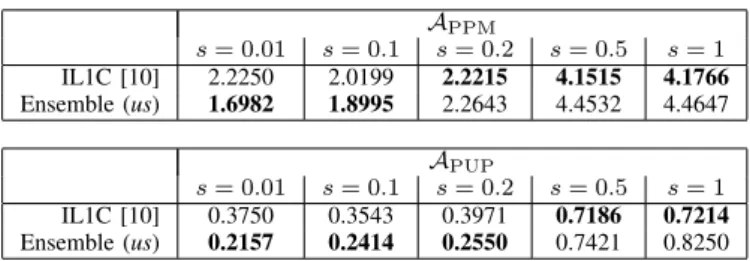
Results & Discussion. The reader can refer to Table IV for the quantitative evaluation of our ensemble strategy applied to IL1C [10] evaluated in the test-case N = 10. We are expecting to register a very interpretable phenomenon out of a simple strategy such as averaging multiple candidate solutions corresponding to the same AIR: we should expect to register a regularizing effect which smooths out the AIRs, removing spurious peaks due to, for instance, numerical instability. This explains the improvements achieved from our proposed ensemble mechanism versus the IL1C [10] baseline: once spurious peaks have been removed, we expect that a peak finding algorithm such that the one applied in [10] can be more effective in finalizing the estimate of TDOAs. This consistently happen in the cases s= 0.01, s= 0.1 (for both APPM and
APUP) ands= 0.2(only forAPUP), while, when considering
the “more difficult” cases s= 0.5 ands= 1we do not see a sharp improvement of the ensemble method. This is probably
TABLE IV
THE ENSEMBLE MECHANISM. WE THE REPORT THE PERFORMANCE OF
IL1C [10] (N= 10,white noise)VERSUS THE ENSEMBLE MECHANISM IN WHICH COUPLES OF MICROPHONES ARE SOLVED,FIRST,AND THE AGGREGATED BY AVERAGING ACROSS THE REDUNDANCY OFAIRS
REFERRING TO THE SAME MICROPHONES. WE DENOTE A BETTER PERFORMANCE IN BOLD,ACROSS DIFFERENT SIGNAL-TO-NOISE VALUES
s. APPM s= 0.01 s= 0.1 s= 0.2 s= 0.5 s= 1 IL1C [10] 2.2250 2.0199 2.2215 4.1515 4.1766 Ensemble (us) 1.6982 1.8995 2.2643 4.4532 4.4647 APUP s= 0.01 s= 0.1 s= 0.2 s= 0.5 s= 1 IL1C [10] 0.3750 0.3543 0.3971 0.7186 0.7214 Ensemble (us) 0.2157 0.2414 0.2550 0.7421 0.8250
due to the fact that the candidate solutions that are averaged are, each of them, noisier. Therefore, the averaging effect produces an excessive over-regularization which excessively smoothens the peaks, damaging the performance of the peak finding. Nevertheless, the regularizing effect of averaging can be inspirational for practitioners in exploiting a large number of microphones to better estimate TDOAs.
VI. CONCLUSIONS
In this work, we generalized the traditional experimental playground in which the notion of cross-correlation identity (CCI), applied to the estimation of TDOAs using blind channel deconvolution methods [10], [11], [14], [17], [18], switching from the caseN = 2toN >2. Our analysis shows that, by simply allowing for a increased number of microphones, the very same state-of-the-art method ILC1 [10] can be sharply boosted in performance (see Tab. III) without requiring any change in the computational pipeline.
We deem that our findings open up to a novel research trend in which CCI identities are better combined with the
case N > 2, so that improvements in the error metrics can
come from two different, yet complementary, factors: advances in the optimization standpoint and multiple CCI relationships. We warm-up the research efforts in this directions with two simple modifications of IL1C, showing that, with respect to an incremental addition of the microphones, the practitioners should preferred a late fusion ensemble mechanism - which has the understandable property of easing the peaks finding-based inference stage of [10].
REFERENCES
[1] Terence Betlehem and Thushara D. Abhayapala, ”A modal approach to soundfield reproduction in reverberant rooms”,2005 IEEE International Conference on Acoustics, Speech, and Signal Processing, ICASSP ’05, Philadelphia, Pennsylvania, USA, March 18-23, 2005, pp. 289–292 [2] I. Dokmani´c, R.Parhizkar, A. Walther, Y. M. Lu, and M. Vetterli,
”Acoustic echoes reveal room shape”, Proceedings of the National Academy of Sciences, 2013, volume 110, no. 30, pp. 12186–12191, National Acad Sciences
[3] F. Antonacci, J. Filos, M. R. Thomas, E. A. P. Habets, A. Sarti, P. A. Naylor, and S. Tubaro, “Inference of room geometry from acoustic impulse responses”Audio, Speech, and Lang. Proc., IEEE Trans. on, vol. 20, no. 10, pp. 2683–2695, 2012.
[4] F. Ribeiro, D. Florˆencio, D. Ba, and C. Zhang, “Geometrically con-strained room modeling with compact microphone arrays” Audio, Speech, and Language Processing,IEEE Transactions on, vol. 20, no. 5, pp. 1449–1460, 2012.
[5] A. H. Moore, M. Brookes, and P. A. Naylor, “Room geometry estimation from a single channel acoustic impulse response”, inSignal Processing Conference (EUSIPCO), 2013 Proceedings of the 21st European. IEEE, 2013, pp. 1–5.
[6] M. Crocco, A. Trucco, V. Murino, and A. Del Bue, “Towards fully uncalibrated room reconstruction with sound,” in22nd European Signal Processing Conference (EUSIPCO), Lisbon, Portugal, 2014.
[7] M. Wu and D. Wang, “A two-stage algorithm for one microphone rever-berant speech enhancement”,Audio, Speech, and Language Processing, IEEE Transactions on, vol. 14, no. 3, pp. 774–784, 2006.
[8] Y. Lin, J. Chen, Y. Kim, and D. D. Lee, “Blind channel identification for speech dereverberation usingl1-norm sparse learning,” inAdvances in Neural Information Processing Systems, 2007, pp. 921–928. [9] K. Lebart, J.M. Boucher, and P. Denbigh, “A new method based on
spectral subtraction for speech dereverberation,”Acta Acustica united with Acustica, vol. 87, no. 3, pp. 359–366, 2001.
[10] M. Crocco and A. Del Bue, ”Estimation of TDOA for room reflections by iterative weightedl1constraint,”2016 IEEE International Conference on Acoustics, Speech and Signal Processing (ICASSP), Shanghai, 2016, pp. 3201–3205.
[11] L. Tong, G. Xu, and T. Kailath, “Blind identification and equalization based on second-order statistics: a time domain approach”,Information Theory, IEEE Transactions on, vol. 40, no. 2, pp. 340–349, Mar 1995. [12] W. Rudin et al.,Principles of mathematical analysisMcGraw-hill New
York, 1964, vol. 3.
[13] J. B. Allen and D. A. Berkley, “Image method for efficiently simulating small room acoustics,”The Journal of the Acoustical Society of America, vol. 65, no. 4, pp. 943–950, 1979.
[14] Y. Lin, J. Chen, Y. Kim, and D. Lee, “Blind sparse nonnegative (bsn) channel identification for acoustic time-difference-of-arrival estimation,” inApplications of Signal Processing to Audio and Acoustics, 2007 IEEE Workshop on, Oct 2007, pp. 106–109.
[15] M. Crocco and A. Del Bue, “Room impulse response estimation by iterative weighted l1 norm,” in 23nd European Signal Processing Conference (EUSIPCO), Nice, France, 2015.
[16] M. Yu, W. Ma, J. Xin, and S. Osher, “Multi-channel l1 regularized convex speech enhancement model and fast computation by the split bregman method”, Audio, Speech, and Lang. Proc., IEEE Trans. on, vol. 20, no. 2, pp. 661–675, Feb 2012.
[17] Y. Lin, J. Chen, Y. Kim, and D. D. Lee, “Blind channel identification for speech dereverberation usingl1-norm sparse learning,” inAdvances in Neural Information Processing Systems, 2007, pp. 921–928. [18] K. Kowalczyk, E. Habets, W. Kellermann, and P. Naylor, “Blind system
identification using sparse learning for tdoa estimation of room reflec-tions”,Signal Processing Letters, IEEE, vol. 20, no. 7, pp. 653–656, July 2013.
[19] L. Benvenuti and L. Farina, “A tutorial on the positive realization problem,”Automatic Control, IEEE Transactions on, vol. 49, no. 5, pp. 651–664, 2004.
[20] D. D. Lee and H. S. Seung, “Algorithms for nonnegative matrix factorization,” inAdvances in neural information processing systems, 2001, pp. 556–562.
[21] M. Krekovi´c, I. Dokmani´c and M. Vetterli, ”EchoSLAM: Simultaneous localization and mapping with acoustic echoes,” 2016 IEEE International Conference on Acoustics, Speech and Signal Processing (ICASSP), Shanghai, 2016, pp. 11-15.
[22] U. Klein and Tr`ınh Qu˜oc V˜o , Direction-of-arrival estimation using a microphone array with the multichannel cross-correlation method, IEEE International Symposium on Signal Processing and Information Technology, 2012.
[23] L. Wang, T. Hon, J. D. Reiss and A. Cavallaro, Self-Localization of Ad-Hoc Arrays Using Time Difference of Arrivals, in IEEE Transactions on Signal Processing, vol. 64 (4), pp. 1018-1033, 2016.
[24] S. H. Shin, K. M. Jeon, N. K. Kim, H. K. Kim, J. E. Lim and J. Park, Coordinate-based direction-of-arrival estimation method using distributed microphones, IEEE International Conference on Consumer Electronics (ICCE), 2018