Municipal Bonds: One Market or Fifty?
Paul Schultz*
October, 2012
Preliminary, do not quote.
Mendoza College of Business Administration, University of Notre Dame. I am grateful to Paul
*
Gao, Chuck Trzcinka, and to workshop participants at the University of Notre Dame and the Federal Reserve Board for comments and suggestions.
1. Introduction
The municipal bond market is large. According to the Securities Industry and Financial Market Association, there were $3.7 trillion worth of municipal bonds outstanding as of 2011. Cities, states, counties, school districts and other government entities issued $294 billion in municipal bonds in 2011, down from $433 billion in 2010. It is not clear though, whether1
municipals represent one large integrated market, or whether it is more accurately characterized as a set of separate markets for investors from different geographic areas.
There are a number of reasons why the municipal bond market may be geographically segmented. First and foremost, most states exempt interest income from municipal bonds issued in the state from state income tax, but do not extend the same tax benefit to bonds from out-of-state issuers. Differences in tax treatments of in-out-of-state and out-of-out-of-state bonds mean that significant differences in before tax yields across states are possible without giving investors an incentive to purchase out-of-state bonds. For example, if investors in a state face a marginal tax rate of 5%, out-of-state bonds must yield more than 5.25% before investors will prefer them over in-state bonds that yield 5%.
This is a major reason for segmentation of the municipal bond market, and the one that is studied here. There are, however, other factors that may contribute to segmentation. Municipal bond issuers are, of course, associated with a particular location. This is different from corporate bond issuers who will sell products all over the country and may have plants, retail locations or other facilities in numerous locations. Investors only have first-hand knowledge of municipal issuers that are located nearby. Municipal issuers are notorious for providing financial
information irregularly - often only when another bond issue is contemplated. Hence investors may prefer local bonds because the soft information about a bond issuer that is available to nearby investors may be the best information available.
In addition, some underwriters of municipal bonds do all or a majority of their business in one state or a few neighboring states. For example, Ameritas Investment was lead underwriter for
1,901 municipal bond issues over 1999 through June 2010. 1,893 of these bonds were from Nebraska. First Midwest underwrote 956 Illinois municipal bond offerings over 1999 - June 2010, and one offering from another state. This geographic specialization of municipal bond underwriting may be both a cause and consequence of market segmentation. 2
Finally, the Securities and Exchange Commission (SEC) has no direct authority over the municipal bond market. It can indirectly influence the municipal market to the extent that it has regulatory authority over municipal bond dealers. Regulatory responsibility rests primarily with the states.
In this paper, I test whether the municipal bond market is segmented by state. A comparison of trade times for bonds by state of issue suggests that in-state investors provide a disproportionate amount of the trading of municipal bonds. What is of most interest of course is not whether ownership or trading of the bonds is segmented, but whether bond prices or yields differ as a result os the segmentation.
I examine differences in yields to maturity across states over two periods. The first, 1999 - 2006, represents a “normal” period for municipal bonds. The second period, 2007 - June, 2010 includes the financial crisis and the collapse of the bond insurers. I use both characteristic matching and regressions to adjust for differences in bond characteristics across states. During the first period, there are significant and persistent differences in yields to maturity across states. There are handful of states that offer no tax advantage to home state issuers. These include states like Texas that do not tax interest on either in-state or out-of-state bonds, and states like Illinois that tax both. Bonds issued in states with no home state tax advantage cannot offer yields less than out of state bonds or investors would forego them for the bonds issued in other states. Consistent with this, I find that bonds issued in states with no home state tax advantage consistently offer higher yields than bonds from other states. The difference in yields was approximately 10 basis points over 1999 - 2006.
Municipal bond defaults were very unusual before the financial crisis and risk was thought to be minimal. More than half of municipal bonds were insured and thought to carry
Butler (2008) compares local and national underwriters for municipal bonds and finds evidence that local 2
virtually no risk. It is difficult to attribute differences in yields across states to differences in risk over 1999 - 2006, especially since I control for differences in Moody’s and Standard and Poor’s ratings.
Default risk took on new importance from 2007 through 2010. In 2005, an uninsured bond that carried the lowest investment grade rating from Moody’s and Standard and Poor’s had a yield to maturity approximately 75 basis points greater than a similar bond hat carried the highest rating from both agencies. By the first quarter of 2009, the difference in yields had grown to 279 basis points.
During the 2007 - June, 2010 period, differences in yields were often much larger. Yields on bonds from Michigan, Louisiana, and particularly California were high. At times during 2009, even after adjusting for differences in bond ratings, bonds from these states had yields that were 50 basis points higher than yields of similar bonds from Massachusetts, Maryland, and some of the smaller states. It seems likely that some of that difference in yields is due to differences in default risk that is not reflected in ratings. Nevertheless, during the crisis period, bonds from states with no home-state tax advantage continued to carry higher yields than bonds from other states.
The market segmentation described here offers several disadvantages over a fully integrated market. Some bond issuers will be forced to pay higher interest rates than they would in an integrated market. Investors may concentrate all of their municipal bond holdings in one state and lose any benefits of geographic diversification, although these benefits seemed small until recently. Finally, investors may be forced to buy bonds with features (maturity, rating, insurance, etc.) that are less desirable than could be found in bonds in a fully integrated market.
This paper complements a recent study by Pirinsky and Wang (2011). They employ a sample of 2001 - 2007 municipal bond offerings from the Thomson Financial SDC Platinum database. They use investment income per capita in a state as a measure of in-state demand for municipal bonds. They use new debt per capita in a state, measured as the municipal bonds issued in the state that year, as a measure of the supply of municipal bonds. Regression estimates suggest that these measures of supply and demand affect yields of municipal bonds in the
out-of-state bonds from state income tax, their measures of in-state municipal bond supply and demand do not have significant affects on yields. Pirinsky and Wang also observe that taxable municipal bonds are less likely to trade in a segmented market than tax exempt bonds that are likely to be purchased mainly by in-state investors. Consistent with this, they find that tax free municipal bond yields are inversely related to a state’s investment income per capita (their measure of demand for bonds) while yields on taxable municipal bonds do not decrease with an increase in in-state investment income per capita. Analogous results are obtained when they use the municipal bonds per capita issued in a state as a measure of the supply of bonds. For tax-free municipal bonds, yields increase with in-state new bonds per capita. Yields of taxable bonds are not affected by recent issues of in-state bonds.
The data used in this paper allow me to do things that cannot be done with Pirinsky and Wang’s data. Their sample is much smaller than the one used here, and consists only of bond offerings. More than three-quarters of the offerings cannot be used because of inadequate
information on yields. Their smaller sample size makes it difficult to examine yields over time or across individual states.
The rest of the paper is organized as follows. The data used here is described in Section 2. Evidence of segmentation from intraday trading volume is provided in Section 3. The next
section provides evidence of market segmentation over 1999 - 2006. Municipal bond yields during the financial crisis are examined in Section 5. Section 6 summarizes and concludes.
2. Data
The data used in this paper comes from three sources. The Municipal Securities
Rulemaking Board (MSRB) supplies data on all municipal bond trades from 1999 though June, 2010. Each trade record contains the time and date of the transaction, the CUSIP number of the bond, the price and yield to maturity of the bond, the par value of the bonds in the trade, and whether the trade was a purchase of bonds buy an investor from a dealer, a sale of bonds from an investor to a dealer, or an inter dealer trade. The MSRB municipal bond trade data has been used
in a number of recent studies, including Harris and Piwowar (2006), Green, Hollifield and Schürhoff (2007a), Green, Hollifield and Schürhoff (2007a), and Schultz (2012) .
Bond characteristics are obtained from the Mergent/FISD fixed income securities
database. Municipal bond issues usually consist of a number of bonds with different maturities. 3
Mergent/FISD provides the offering date, underwriter, issuer state, and total amount offered for issues. For individual bonds, Mergent/FISD provides the coupon, maturity date, offering price, debt type (general obligation, revenue, etc.), codes for whether the bond is putable or callable, the insurance provider (if any), and Moody’s, Standard and Poor’s, and Fitch ratings and rating dates. These ratings are the most recent ratings as of the time the Mergent/FISD data was purchased in 2010.
The third data set consists of all changes in Moody’s ratings of municipal bonds over 1999 - June, 2010. This is combined with the Moody’s ratings from Mergent/FISD to provide the Moody’s rating in effect for a bond at the time of each trade. The three data sets are combined using CUSIP numbers.
Firm quotes, or even indicative quotes, are unavailable for municipal bonds. Hence to study municipal bond yields, I must use the yields implied by trade prices. To minimize issues related to trading costs or intermediation, I use only purchases of bonds by investors from dealers to compare yields. Municipal bonds are infrequently traded. A large portion of the trades are associated with the original sale of the bonds.
In total, there are 36.2 million purchases of tax-exempt fixed-rate bonds by investors from dealers in the data set. Panel A of Table 1 provides some summary statistics for the trades for each year from 1999 - June, 2010. The mean time to maturity at the time of the trades ranges from a low of 11.93 years in 2006 to 15.83 years in 2001. The median size trade is $25,000 par value most years, but reaches $30,000 in 2006 and 2007. In most years the 25 percentile of tradeth
size is $10,000 and the 75th percentile is $50,000. The 25 and 75 percentiles of trade size areth th
somewhat larger over 2005 - 2008. Most purchases are small purchases by retail investors. The median yield to maturity ranges from 3.67% in 2005 to 5.25% in 2000. The
interquartile range is as small as 87 basis points in 2000 and as large as 202 basis points in 2009. This range depends on the variation of yields across bonds on a specific date, and the variation of yields over the year.
The next line shows the proportion of trades that are in insured bonds. These bonds are thought to be more liquid than uninsured bonds, so it is likely that they trade more frequently. Hence the proportion of trades in insured bonds is likely to be slightly larger than the proportion of bonds that are insured. Insurance purchases dropped of dramatically for new issues of bonds after 2007, so it is not surprising that the proportion of trades in insured bonds falls sharply toward the end of the sample period.
General obligation bonds make up between 26.6% and 37.5% of the trades. The majority of the bonds that trade in any year are callable. A sizeable proportion of the bond trades were in “new issues,’ bonds that were issued no more than two months before. In 2000, the lowest proportion of trades, 23.5%, were in new issues. The highest proportion, 43.2%, occurred in 2002.
Panel B provides the average number of trades per day over 1999 - June, 2010 for the 25 most populous states, and for all others. The average is 1,762.8 for California, 1,307.2 for New York, 832 for Texas, and 1,955.3 for all states outside of the 25 most populous. With 2,883 trading days over 1999 - June, 2010, There are over 5,000,000 trades of California bonds, 3.8 million trades of New York bonds and 2.4 million trades of Texas bonds.
3. Segmentation: Evidence from Intraday Trading Volume
If municipal bonds are traded exclusively in state, we would expect intraday trading patterns to be affected by the time zone of the state. When it is 9:30 am on the East Coast, we would expect more trading volume in bonds issued by Eastern states than in bonds issued by Pacific Coast states where the time is only 6:30 am. Conversely, when it is 12:30 Eastern Time, we would expect little trading in bonds issued on the east coast as traders and investors break for lunch. It would be only 9:30 on the West Coast though, and we would expect heavier volume in bonds issued by cities in the Pacific time zone. On the other hand, if all municipal bonds were
equally likely to be traded all over the country, we would expect to see similar intraday trade patterns regardless of the geographic origin of the bond.
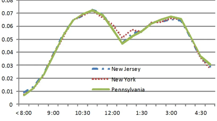
I calculate the proportion of all buy orders for municipal bonds for each state that take place during every half-hour interval from 8 am to 5 pm Eastern Time over 1999 - June, 2010. Figure 1a depicts the proportions for three Eastern states: New Jersey, New York, and
Pennsylvania. Intraday patterns are similar for bonds from each state. Volume rises steadily from 8 am to 11 am. It declines sharply from 11:30 to 12:30 as investors and bond dealers head to lunch, and then rises again until 3 pm. Volume then falls until the close.
Figure 1b shows the proportion if intraday volume in each Eastern Time half hour period for bonds from three Pacific states: California, Oregon, and Washington. Intraday trading
patterns are very similar for bonds from each of the Pacific states, but very different from patterns for bonds from Eastern states. These bonds have a smaller portion of their volume in in the early morning than do bonds from the Eastern states. Their trading volume peaks when it is 1pm on the East Coast and investors there are still at lunch. Volume spikes near 5pm for West Coast bonds, while it declines for East Coast bonds.
Figure 1c contrasts the patterns of intraday trading for New York, Texas, and California. When plotted together, it is obvious that the patterns are very different. It is interesting that the proportion of trades of Texas municipal bonds is similar to that of New York bonds one hour earlier. Almost all of Texas is in the central time zone, one hour earlier than New York’s eastern time zone.
These differences in intraday trading patterns suggest that municipal bonds are traded primarily by investors in the time zone of the issuer. It seems likely that bonds are traded primarily in the state in which they are issued, and perhaps in the municipality that issues them, but these intraday trading patterns do not provide direct evidence on this issue.
Of course, even if the great majority of municipal bonds are purchased by in-state investors, the municipal bond market need not be segmented by state. A small number of
investors, operating across state lines, can keep yields in line. I now turn to testing whether bond yields differ across states.
4. Market Segmentation Over 1999 - 2006
I split the sample period into two separate subperiods to examine market segmentation in yields. The first, 1999 - 2006, represents a ‘normal’ period. During this time, default risk was thought to be minimal for municipal bonds. About half of bonds were insured by AAA rated insurers. The second subperiod, 2007 - June, 2010, includes the financial crisis. Bond insurance, which was thought to make the market more liquid, was purchased by few issuers as the insurers themselves were downgraded.
4.1 Evidence from Bond Yields of Matched Trades
Even if most trading in municipal bonds is concentrated in the state of their issue, a few trades by sophisticated investors can keep bond yields the same across states. On the other hand, if taxes and other market frictions provide significant advantages to investing in-state, municipal bond yields may differ significantly across states.
I first employ a matching procedure to see if bonds issued in different states have different yields. Each day I match purchases of bonds from each of the ten largest population states with purchases of bonds from the other 40 states, Washington D.C., and Puerto Rico. The ten largest population states (California, New York, Texas, Florida, Illinois, Pennsylvania, Ohio, Michigan, Georgia, North Carolina) are compared with the others because each of the ten has enough trades to ensure a large number of matches. For a large state bond trade to be matched with the trade of a bond from another state, the two trades 1) must be purchases of bonds by investors from dealers, 2) must both occur on the same day, 3) must be purchases of the same par value of bonds, 4) must mature with 0.04 years (two weeks) of each other, 4) must have coupon yields that differ by 25 basis points or less, 5) must be of bonds that or both callable or not callable, 6) must be of bonds that are both ranked as investment grade by Moody’s. Each trade is used in only one match. So, if a purchase of a small state bond is matched with the trade of a New York bond, it will not be matched with any other New York bond trades or any California bond trades either. This methodology results in 996,496 matched bond trade pairs, or on average,
a little less than 50 per large state per day. While the total of almost 2,000,000 trades is a large sample, it is derived from the much larger total of over 23,000,000 trades during the same period.
In matching, I only require that both bonds have investment grade ratings because an exact match of Moody’s ratings reduces the number of matched trades by about 75%. Defaults of municipal bonds are far less common than defaults of corporate bonds, and ratings differences are associated with smaller differences in yields. Nevertheless, for each day, I regress the
differences between bond yields of large states and their small state matches on the differences in their Moody’s rankings. Differences in Moody’s ratings are the number of “notches” between them. So, for example, the difference between an Aa3 and an Aa1 ranking is two. I use the intercepts of the regression as measures of the excess bond yield for the large state on that day.
The excess bond yields for California bonds for 1999 - 2006 are graphed in Figure AA. The yields are expressed in percentages, so an excess yield of 0.1 represents a yield that is ten basis points above the yield of matching bonds. The excess yields of California bonds are
consistently negative in 1999 - 2000, and less than negative 20 basis points for extended periods. They are positive and generally larger than 10 basis points in 2003 and 2004. The excess yields of Texas bonds are graphed in Figure BB. These excess yields are consistently positive and typically greater than 10 basis points. Investors in Texas bonds receive higher yields than investors in small state bonds.
These results are consistent with a segmented market for municipal bonds. Alternatively, it could be argued that these results reflect deficiencies of the matching procedure. The matching methodology controls very well for some of the important determinants of municipal bond yields, particularly trade size and time to maturity. On the other hand, in order to maintain a reasonable sample size, I do not control for some other variables associated with yield. It seems unlikely that differences, for example, in the use of bond insurance or differences in the proportion of general obligation bonds across states could be so large and so consistent as to explain the excess yields of these bonds. Nevertheless, I adjust for a number of other yield determinants using a regression methodology later in the paper.
I use a Fama-MacBeth methodology to test whether the excess yields of the bonds from the ten largest states are different from zero. Recall that for each large state each day, I regress
the difference between the yield on the large state bond trade and the yield on the matching trade on the difference in the Moodys rankings of the two bonds. The intercept term is a measure of the excess yield of municipal bonds of that state. Then, I assume the excess yields follow and AR(1) process and estimate the constant, the AR(1) parameter and their standard errors. The constant term is an estimate of the average excess yield of bonds issued in that state. I estimate the average excess returns separately for the two halves of the sample period: 1999 - 2002 and 2003 - 2006. These estimates are reported in Table 2.
In the first subperiod, all ten of the large states have excess yields that are significantly different from zero at a one percent confidence level. In the second subperiod, excess returns are significantly different from zero at the one percent level for eight of the ten large states. Over 1999 - 2002 four of the large states have municipal bond yields that are smaller than the yields of the small states, while six of the ten have municipal bond yields that exceed small state yields. Over 2003 - 2006, six of the states’ bonds have yields that are smaller than the small state controls, while four have larger yields. Both Texas and Illinois bond yields are about ten basis points more than the yields of small state bonds in both periods. There are no state tax
advantages to buying in state bonds in either Texas or Illinois. Texas has no state income tax, and Illinois taxes interest on both in-state and out-of-state municipal bonds. Hence Issuers in both of these states cannot offer low yields and expect in-state investors to purchase them to avoid state taxes. If yields on Texas or Illinois bonds are low relative to yields of bonds from other states, investors will find it worthwhile to instead purchase out-of-state bonds.
California is unusual in that excess yields on California bonds are, on average -0.1237 over 1999 - 2002 but switch signs to 0.0240 over 2003 - 2006. These averages conceal a lot of variation in California bond yields over the subperiods. Figure AA shows that California bond yields were more than 20 basis points below small state yields for extended parts of 1999 - 2002, and more than 10 basis points above small state yields for long stretches of 2003 - 2006.
Table 2 provides time series means of the intercept coefficients from the daily regressions of the difference in yield to maturity for matched bond trades on differences in Moody’s ratings. Table 3 reports the proportion of individual day intercepts that are more than two standard deviation above or below zero for each state each year. For California, a large portion of the
individual day regression intercepts are significantly less that zero over 1999 - 2002. In 2000, the intercept coefficient had a t-statistic less than -2 in more than 96% of the individual day
regressions. On a specific day it may be possible to argue that the lower yields of California bonds are due to an inadequate matching procedure. When California bonds offer significantly lower yields on 96% of the trading days, while the specific bonds traded change daily, it seems clear that the state of issue affects the yields.
In California, the low yields on bonds eventually disappeared. In 2003 and 2004, t-statistics of more than 2 occurred on many days for California bonds. Yields on California municipals were frequently significantly greater than yields on matched bonds.
Results for Texas are shown in the last two rows of Table 3. In each year, 0.4% or fewer of the intercept coefficients have t-statistics less than -2. In every year, at least 30%, and in two years more than 70% of the daily intercept coefficients have t-statistics > 2. The yields on Texas bonds are consistently higher than yields on matched bonds.
The results from matched trades lead to two conclusions. First, the municipal bond market does appear to be segmented by state. Bonds from some large states offer yields that are consistently higher than yields on small state bonds. Bonds from other large states offer yields that are consistently lower than similar bonds from small states. Second, bonds from Texas and Illinois, the states that offer no tax advantage to in-state bonds, offer yields that are consistently about ten basis points higher than yields on small state bonds.
Most states offer a state tax advantage to in-state municipal bond issuers. An investor in, say, New York, does not pay state income taxes on a interest on bond issued by a municipality in the state, but does pay state tax on interest from out-of-state bonds. So, unless the yield on the out-of-state bonds is much higher, the New York investor will prefer to invest in New York bonds.
Texas and Illinois are two states that do not provide a home-state tax advantage to municipal issuers. There are several others as well. Alaska, Nevada, South Dakota, Washington and Wyoming, like Texas, have no state income tax and hence no tax advantage for in-state bonds. Wisconsin, like Illinois, taxes interest on both in-state and out-of-state bonds. Hence, for these states there is again no tax advantages to holding in-state bonds. Indiana and Washington
D.C. do not tax interest on either their own bonds or the bonds of out-of-state issuers. These nine states, plus Washington D.C. make up the no home-state tax advantage states.4
Because there are no home state tax advantages for bonds issued in these states, yields cannot be lower than investors could get elsewhere. If yields were low, investors in that state would be happy to buy out-of-state bonds with higher yields. Hence it is not surprising that yields of bonds from Illinois and Texas are, on average, higher than yields of matching bonds.
The tax treatment of bonds from issuers in U.S. Territories - Puerto Rico, the Virgin Islands, and Guam - provide an interesting contrast. They are exempt from state income tax in every state. If these bonds offered abnormally high yields, they would be purchased by investors all over the country. Therefore, bonds from U.S. Territories should not have high yields, and may, on average, have lower yields than similar bonds from most states.
I next test whether yields of bonds from states with no home-state tax advantage and bonds from U.S. Territories provide different yields than bonds from the majority of states with a home-state tax advantage. The matching procedure used up to this point has limitations. Most trades are not matched. In addition, bonds from U.S. Territories have relatively few trades. It is difficult to estimate a yield premium for bonds from the Territories when most of the trades are not matched. So, to test whether bonds from states without a home-state tax advantage have higher yields, and bonds from issuers in U.S. Territories have lower yields, I use regressions to estimate excess yields after adjusting for other factors.
4.2 Using Regressions to Determine the Yield to Maturity on a Purchased Bond
For the rest of the paper, I use cross-sectional regressions with bond characteristics and dummy variables for states to test whether the state of issue is a determinant of yield after adjusting for other bond characteristics. This is similar to the approach taken by Bergstrasser, Cohen, and Shenai (2011). They look at the impact of fractionalization of county population
Florida did not have a state income tax, but until January 2007 they had an intangible
4
personal property tax on the value of asset holdings that they applied to out-of-state but not in-state bonds.
makeup and its impact on bond yields in offerings. Fractionalization is measured as 1 minus the Herfindahl index for religious or ethnic groups. Bond characteristics that Bergstrasser, Cohen, and Shenai find significant in explaining muni yields include log of issue size and log of bond size, dummies for competitive and negotiated issues, bond insurance, callable and puttable dummies, and a GO bond dummy. They use separate dummy variables for each maturity month.
For every day from 1999 through 2006, I run cross-sectional regressions with the yield to maturity as the dependent variable. Observations consist of every trade that day in which an investor purchased at least $25,000 and less than $10,000,000 (par value) of tax exempt municipal bonds from a dealer. Yields differ significantly for different maturities, so I include only trades of bonds with three to 25 years until maturity. The regression for the yield on purchase i is
Table 4 reports the mean, 25 percentile, and 75 percentile of each coefficient and t-th th
statistic from the daily cross-sectional regressions. The second and third variables are No Home State Adv and U.S. Territory. These are the variables of primary interest. The No Home State Adv variable takes a value of one for bonds issued in states with no state tax advantage for in-state bonds. The mean coefficient across days is 0.1070, indicating that bonds from issuers in these states had yields to maturity that were 10.7 basis points greater than yields on bonds issued in states with a tax advantage for in-state bonds. Both the 25 and 75 percentile of coefficientsth th
surprising. If there is no tax advantage to buying in-state municipal bonds, the in-state bonds will not attract in-state investors if yields are low.
The next variable is a dummy variable that takes a value of one if the bond issuer is from a U.S. territory - Puerto Rico, the Virgin Islands, or Guam. These bonds are exempt from state taxes in all U.S. states. Hence, if they carried high yields, investors from all over the country would find it worthwhile to invest in these bonds. It is therefore not surprising that the mean, 25th
percentile, and 75 percentile of the coefficients are negative. The mean and 75 percentile of theth th
t-statistics indicate that the coefficients on individual day regressions are usually not significant. This is not surprising. There are just not that many bonds issued from these territories.
The next three variables are time to maturity, inverse of time to maturity, and the natural logarithm of time to maturity. I include all three to capture any non-linearities in the relation between time to maturity and yield. Typically, the coefficient on time to maturity is negative, while the coefficient on the inverse of time to maturity is positive and the coefficient natural logarithm of the time to maturity is positive and significant. When the time to maturity is used without its transformations, the coefficient is typically positive and significant.
I also use both trade size and log of trade size and issue size and log of issue size to capture non-linearities in the relation between yield to maturity and these variables. Trade size is included to capture fixed costs of trading and negotiating power and ability of larger investors. Coefficients on trade size are generally positive, while coefficients on the natural log of trade size are consistently negative and significant. Issue size is a proxy for liquidity, with larger issues associated with greater liquidity. Longstaff (2011) suggests that much of the municipal puzzle, that is the finding that marginal tax rates implied by municipals are low, may be due to the liquidity premium embedded in municipal prices. Wang, Wu, and Zhang (2008) examine the impact of liquidity risk on municipal bond yields using bond transactions from the MSRB
database for July 2000 through June 2004. Their results suggest that liquidity risk affects returns, particularly for low rated bonds and bonds with a long-time to maturity. Coefficients on both issue size and the natural log of issue size are usually negative, which is consistent with the joint hypothesis that size proxies for liquidity and greater liquidity is associated with lower yields.
-general obligation bonds, tobacco bonds, loan agreements, and “doubled barreled” bonds . General obligation (GO) bonds are backed by the full taxing power of the state, county, or municipality rather than the being paid from the revenues of a specific bridge, parking ramp, or other project. Traditionally, they are thought to be among the safest municipal bonds. The mean coefficient on the GO bond dummy is -0.0811, with a t-statistic of -3.23. The 25 and 75th th
percentiles of the GO coefficient are also negative and significant at the 5% level. Tobacco bonds are paid with revenues from tobacco settlements. In general, the coefficients on the dummy variables for tobacco bonds are positive. The coefficients on the loan agreement dummy
variables are typically positive. Double barreled bonds are backed by more than one entity - say a school district and a county. Coefficients on on the double barreled bond dummy are usually negative.
Many municipal bonds, particularly those with more than ten years to maturity when issued, are callable. We would expect these bonds to carry higher yields to compensate for the risk of being called if interest rates fall. The mean coefficient on the dummy variable for callable bonds is 0.2207, suggesting that these bonds have yields that are 22 basis points higher than non-callable bonds, all else equal. The 25 and 75 percentiles of the non-callable dummy variable areth th
negative and significant at the 5% level.
Putable bonds can be put to the issuer at the bond’s par value. They are somewhat
unusual. Fewer than 2% of sample purchases are of putable bonds. The ability to put the bonds if interest rates rise is valuable to investors, and we would expect them to have a lower yield. The mean coefficient is -1.2473, indicating that putable bonds have yields that are more than 124 basis points less than similar bonds. Both the 25 and 75 percentile coefficients are negative andth th
statistically significant at the 1% level.
The premium dummy takes a value of one if the bond is selling for a higher price then its issue price. The mean coefficient is positive and but insignificantly different from zero. The impact of call provisions on a bond price is complex, and depends on the likelihood the bond will be called, the existence of a no call period and other factors. Clearly, using just a dummy variable for a call provision cannot completely capture its effect on yields. I also include in the regressions an interaction between the dummy variable for premium and the call provision dummy variable.
This coefficient on this variable is generally negative and highly significant.
Insured is a dummy variable that has a value of one if the bond is insured. Insurance is purchased by the issuer when the bonds is offered to the public. The issue pay a single fee at the time of issuance, and the insurance company agrees to make any future principle and interest payments that would otherwise be missed. The issuer expects to make up the up front costs of the insurance with lower interest payments. The mean coefficient for insured is -0.4752, implying that insured bonds offer yields to maturity that are 47 ½ basis points lower than similar uninsured bonds. Both the 25 and 75 percentiles of the coefficients on insured are negative. The 25 andth th th
75 percentiles of the t-statistics a high degree of statistical significance. On the great majority ofth
days, insured bonds provide lower yields.
The next two variables are interaction terms between the insured dummy variable and dummy variables for an investment grade rating by Moody’s and an investment grade rating by Standard and Poor’s. The coefficients on the interaction between Insured and an investment grade rating from Moody’s are generally positive and significant. Much of the benefit from insurance is lost when bonds are already highly rated. The interactions between Insured and an investment grade rating from Standard and Poor’s are generally insignificant. These two interaction terms are highly correlated however.
The next variable in the regressions is New Issue, a dummy variable that takes a value of one if the bond was issued less than two months before. The mean of the daily coefficients is 0.1504, indicating that newly issued bonds carry yields that are about 25 basis points greater than more seasoned bonds. Both the 25 and 75 percentiles of coefficients are positive. More than 75th th
percent of the New Issue coefficients in the daily regressions are significant at the one percent level.
The variable Deminimus is a dummy variable that takes a value of one if the trade price of the bond is more than 25 basis points times the number of years to maturity less than the offer price of the bond. Coupon payments on municipal bonds are free from federal income tax, as are capital gains from original issue discount bonds. If, however, a bond is purchased in the
secondary market for a price below the reoffering price, that additional gain is taxable. Far bonds issued at par, the gain is ignored for tax purposes if the discount to the reoffering price is less
than deminimus level of 25 basis points times the number of years to maturity. The rule is similar for original issue discount bonds. These tax issues are described thoroughly in Ang, Bhansali, and Xing (2010). The dummy variable is intended to capture the existence of gains that are not exempt from federal taxes. We would expect such bonds the have higher yields than others. The mean coefficient of 0.6152 indicates that these bonds do indeed have higher yields to maturity. On more than 75 percent of the days in the sample period, the Deminimus coefficient is
significant at the one percent level.
I next include dummy variables for each of the Moody’s investment grade bond ratings, a dummy variable for Moody’s ratings that are below investment grade, and a dummy variable for no rating from Moody’s. These dummy variables provide a comparison of yields with Moody’s Aaa rated bonds. The Mergent data includes the most recent rating by Moody’s as of the date the Mergent data was cut, in the summer of 2010. Bonds that traded, say in 2000, may well have had ratings changes by 2010, or when they matured. I obtain a data set from Moody’s of all ratings changes in all municipal bonds for 1999 - 2010. The data set contains CUSIP numbers of bonds with ratings changes, dates of changes, ratings on the underlying security, on the insured security, and enhanced ratings before and after the ratings change. This allows me to construct a
contemporaneous rating for each underlying bond at the time of each trade. If the bond rating did not change over 1999 - 2010, I use the last rating from Mergent to determine the bond rating at the time of the trade.
I use a similar dummy variables for Standard and Poor’s ratings. S&P ratings are from Mergent and are the most recent rating as of July 2010. Unlike the Moody’s rating, this rating may not have been in effect at the time of a trade.
Mean coefficients on all of the ratings dummies are positive. This is not surprising. It just indicated that all bond without top ratings (AAA or Aaa) have higher yields. For bonds with lower investment grade ratings from Moody’s, mean yields are more than 30 basis points greater than yields of Aaa bonds. Likewise, bonds with S&P ratings of BBB or BBB- had mean yields that were 35 basis points lower than AAA bonds. Note that bonds with the lowest investment grade rating from both Moody’s and Standard and Poor’s had mean yields that were 65 basis points greater than mean yields on bonds that received the highest ratings from both agencies.
Inevitably, there are omitted variables in the regression. All of the determinants of municipal bond yields are not included. Likewise, experimentation would almost certainly allow me to improve the form of the current variables. For example, incorporating features of the call and put provisions rather than just using dummy variables would probably provide more accurate descriptions of yields. Additional interaction terms between, say, ratings and time to maturity might also be useful. The issue though, is whether there are remaining systematic differences between bonds from different states that would explain differences in yields.
4.3. A Comparison of Yields from Bonds With and Without a Home State Tax Advantage
Every day from 1999 through 2006, I run cross-sectional regressions of yield to maturity on a dummy variable that takes a value of one if the bond is issued in a state with no home- state tax advantage, a dummy variable that equals one if the bond is issued from a U.S. Territory, and other variables as described above. When measured either over the entire 1999 - 2006 period or over individual years the time series of coefficients on the no home-state tax advantage variable tends to have a significant, positive first order autocorrelation and slowly declining
autocorrelations for longer lags. So, to test whether the average daily coefficient is different from zero I assume that the time series of coefficients follows an ARMA(1,1) process. Results are reported in Panel A of Table 5.
The first column reveals that the average coefficient on no home-state tax advantage calculated using all days of 1999 - 2006 is 0.1068. All else equal, yields of bonds from states without a home-state tax advantage are more than ten basis points higher than yields of bonds from other states. The z-statistic of 28.54 indicates that the yield difference for states without a home tax advantage is highly significant. This makes sense. If yields were higher in other states, investors in states like Texas, where there is no home state tax advantage, will buy out-of-state bonds. On the other hand, the higher yields will not attract investors from states where there is a home state tax advantage. The extra ten basis point yield would be attractive, but would be cancelled out by the higher state income taxes.
1999 - 2006. There is some year-to-year variation in the yield premium paid by issuers from states with no home-state tax advantage, but every year the mean coefficient is positive and significant. Bonds issued in states without a home state tax advantage have consistently higher yields.
It seems unlikely that the higher yields of bonds from states without a home state tax advantage are due to greater risk. Nevertheless, I rerun the regressions using only insured bonds. Before the 2008 financial crisis, investors had confidence in the companies that insured these bonds. The ratings with the insurance would be Aaa, and the yields reflect the bonds’ perceived safety.
The second column of Panel A reports the average of the daily coefficients on yields of bonds without a home state tax advantage. When the sample is restricted to insured bonds, the average coefficient for the entire period changes only sightly from 0.1068 to 0.1042. The third column reports results when the sample is restricted to trades of uninsured bonds. Over the entire period, uninsured bonds without a home state tax advantage provide yields that are 11.75 basis points higher than bonds with a home state tax advantage. These results suggest that differences in yields between bonds with and without a home state tax advantage are not due to differences in risk.
The next two columns of Panel A provide excess yields for bonds with no home-state tax advantage separately for large ($$100,000 par value) and small (< $100,000 par value trades. It is plausible that large investors are more likely to buy out-of-state bonds to get higher yields. The excess yields, however, are positive and significant for both trade size categories for each year. The last two columns report mean coefficients and z-scores for the no home-state advantage variable for bonds with three to ten years to maturity, and for bonds with more than ten years to maturity. Coefficients on the no home-state advantage dummy are positive and significant for the entire period and each individual year for both short and long-term bonds. The magnitudes of the coefficients are very similar across bonds with short and long maturities.
Panel B is similar to Panel A but reports coefficients for the U.S. Territories dummy variable. As before, an ARMA (1,1) process is fitted to the U.S. Territories coefficients, and the intercept and corresponding z-statistics are reported. When all all bonds issued in U.S. Territories
are included, the intercept coefficient for the entire 1999 - 2006 period is negative and significant as are the coefficients for each individual year. Municipal bonds issued in U.S. Territories
provide lower yields than municipal bonds issued in states. This is not surprising. Since they are exempt from taxes in all U.S. states, they would be purchased by investors thoughout the U.S. if they had high yields. The next two columns report coefficients when only insured and when only uninsured bonds are used. Intercept coefficients from the ARMA (1,1) process are negative and significant in both cases, but tend to be of greater magnitude for the uninsured bonds. A way to interpret this is that uninsured bonds from U.S. states tend to have high yields, while uninsured bonds from U.S. territories do not have particularly high yields. It is possible that only the safest and most liquid bonds from U.S. Territories are uninsured.
The next two columns report results for trade of more than $100,000, and for trades of less than $100,000 (par value) of bonds. Yields for bonds from U.S. Territories are significantly lower than yields for U.S. bonds both for large and small trades. The difference in yields is generally lower for trades of more than $100,000 though.
Results for bonds with three to ten years to maturity are shown in the penultimate column, while results for bonds with more than ten years to maturity are shown in the last column. It appears that the low yields for bonds from U.S. Territories are concentrated in the bonds with longer maturities. For the entire period, yields on bonds from U.S. Territories with more than ten years to maturity are about 24 basis points less than similar bonds from U. S. States with a home-state advantage. The yield differential for the entire period, for bonds with three to ten years to maturity, is indistinguishable from zero.
The regressions have thus far lumped together bonds from all states without a home state tax advantage. It is worthwhile to see if these results are driven by bonds from specific states. I rerun the daily cross-sectional regressions including only the states with a home state tax advantage and one of the states with no advantage. I do this for each of the ten states with no home state tax advantage. I report results for the excess yields of bonds from each of the no advantage states for the entire 1999 - 2006 period in Table 6.
There are a total of 2,007 trading days over the 1999 - 2006 period, but there are not enough trades to estimate the excess yield for each state each day. This is an especially
significant problem for Wyoming, where an estimate of the excess yield can only be obtained on 1,392 out of 2,007 days.
The third column of the table reports the percentage of days with a premium, that is the percentage of days when bonds from the state have a higher yield than bonds from states with a home-state tax advantage. The proportion is greater than 70% for Alaska, the District of
Columbia, Illinois, Indiana, Nevada, South Dakota, Texas and Washington. No state has a proportion less than 50%.
With the exception of Wisconsin and Wyoming, all of the states with no home state tax advantage report a positive time-series mean of the excess yield that is significantly different from zero. Bonds from Alaska yield 19.53 basis points more than bonds from states with a home-state tax advantage all else equal. For South Dakota, the mean excess yield is 16.56 basis points. Wisconsin bonds yield half a basis point more than states with a home state tax advantage, a difference that is not statistically significant. The time series mean of the Wyoming excess yield is -4.47 basis points. It is not clear why Wyoming residents continued to buy their in-state bonds during this period. This is the least populous state, so it is likely that the yields reflect the
decisions of a small number of investors and institutions.
The last two columns report the proportion of the daily regressions in which the t-statistic for the excess yield is less than negative two and more than two. For each state, there are far more days with excess yields that are significantly greater than zero than days when excess yields are significantly less than zero. For Indiana, for example, the t-statistic on excess yield is less than negative two on 0.3% of the days, and greater than positive two on 26.5% of the days. For Alaska, t-statistics for the excess yield are less than negative two for 0.4% of the days and more than two for 47.6% of the trading days.
Although the results for Wyoming are anomalous, the clear result seems to be that yields are higher for bonds issued in states without a home state tax advantage.
To summarize, we have learned three things from examining yields to maturity of
municipal bond from the ‘normal’ period of 1999 - 2006. First, yields do differ based on the state of the issuer. Second, the differences in yields of similar bonds across states are of reasonable magnitude. Yield differences are seldom consistently greater than 20 basis points. Third, tax
treatment of in-state versus out-of-state bonds is a major reason for differences in yields across states. Bonds from states that do not offer a tax advantage for home-state bond have higher yields. Residents of those states can always buy out-of-state bonds if yields on the in-state bonds are low.
4.4 Discussion: The Costs of Market Segmentation
By restricting their municipal bond investments to one state, investors forego many of the benefits of geographical diversification. For the 1999 - 2006 period examined here, these benefits were small. Municipal bond defaults were unusual, and were almost always confined to one municipality or project. In more recent years, the benefits of geographic diversification have increased. The likelihood of default has increased significantly for a number of cities in California, Michigan, and Illinois. Diversifying into out of state bonds can be valuable for residents of these states.
When municipal bond investments are restricted to one state, investors may also have to compromise on other bond characteristics. An investor who wants a 12-year general obligation bond that is not callable and is insured may have a difficult time locating the bond if he restricts his search to, say, Connecticut bonds.
Municipal investors are not, of course, prevented from buying out-of-state bonds. They will buy out-of-state bonds for diversification purposes or to obtain bonds with specific
characteristics. Taxes just make it more costly for them to do so.
If all states exempted interest from out-of-state bonds from state taxation, investors would be better off. It may, however, mean higher interest rates for issuers from states with high
demand for and little supply of bonds.
As we have seen, yields are high on bonds issued in states with no home state tax
advantage. For issuers in these states, yields may decrease if the states start to tax interest on out-of-state bonds. This will create a captive clientele for these bonds that would otherwise invest in out-of-state bonds.
5 Municipal Bonds Yields During the Financial Crisis
Prior to the financial crisis of 2008 - 2009, municipal bonds were considered very safe investments. Defaults were highly unusual. Insurance was purchased by issuers for more than half of bond issues. Default risk became a significant factor starting in 2008. Several bond insurers were downgraded in 2007, which reduced the value of bond insurance. The recession and the steep decline in housing prices cut revenues to municipal bond issuers, and increased the likelihood of default.
For each day, from 2005 through June 2010, I regress yield to maturity for purchased bonds on the same explanatory variables used before, including dummy variables for each Moody’s investment grade bond rating, each Standard and Poor’s investment grade bond rating, ratings below investment grade from each agency, and for no rating from either agency. I also include dummy variables that equal one if the issuer is located in each of the 25 largest population states.
Table 7 shows how the coefficients on the ratings dummies changed over time. I
calculated averages of the daily regression coefficients on ratings dummies for 2005, 2006, and 2007, and for each quarter from 2008 through June 2010. Average coefficients for Moody’s and equivalent Standard and Poor’s ratings are shown in adjacent columns in the table. The daily cross sectional regressions do not have dummy variables for AAA (Standard and Poor’s) or Aaa (Moody’s) ratings, so the coefficients can be interpreted as the extra yield associated with these lower ratings. If the bonds carry equivalent ratings from Moody’s and Standard and Poor’s, the total premium over a bond with AAA and Aaa ratings is obtained by summing the two
coefficients.
Table 7 reveals that yields were only slightly higher for lower rated bonds than bonds that carried the highest ratings in 2005 - 2007. For example, in 2007, the coefficient on the Aa3 rating dummy is 0.0301 and the coefficient on the AA- dummy is 0.0492. Hence a bond rated Aa3 by Moody’s and AA- by Standard and Poor’s would provide a yield that was only 7.93 basis points greater than the yield on an otherwise similar bond that carried the highest rating from
both agencies. In 2007, even the bonds with the lowest investment grade rating from both agencies offer yields that are only 57 basis points greater than the yields on bonds that carry both agencies highest ratings.
From late 2008 on, coefficients on the ratings dummies are much larger. For example, in the first quarter of 2009, the coefficient on the Moody’s Baa3 rating is 1.4228, while the
coefficient for the Standard and Poor’s BBB- rating is 1.3677. Hence a bond with both of these two equivalent ratings would have a yield to maturity that was 2.79% greater than a bond with the highest ratings from both agencies.
Before 2008, the effect of risk on municipal bond yields was small. Differences in risk across states that were not captured by bonds ratings seem highly unlikely to explain differences in yields across states. More caution is required when examining differences in yields across states over 2008 - 2010.
Table 8 reports average coefficients on state dummies for each of the 25 largest
population states for the years of 2005, 2006, and 2007, and for each quarter from 2008 through June 2010. These coefficients can be interpreted as the extra yield for bonds from a particular state over bonds from small population states.
The coefficients for 2005 and 2006 are provided to allow comparison of yields since the crisis with yields from a more normal period. There is more variation in yields across states over 2008 - 2010 than during 2005 - 2006. For example, from the second quarter of 2008 through the second quarter of 2010, California bond yields exceed small state yields by 33 to 39 basis points. This is much larger than any of the state coefficients from 2005 - 2006. The coefficients on Louisiana for the second and third quarter of 2009 indicate that Louisiana bonds had yields more than 40 basis points larger than small state bonds. Michigan and Alabama bonds also carried high yields during this period.
Differences in risk that are not captured by bond ratings are a possible explanation for differences in yields across states. The states with high yields are those that were popularly thought to be especially risky. Otherwise, it would appear that investors in state with no home state tax advantage, like Indiana and Washington, should be purchasing bonds from California, Michigan, and Alabama for their higher yields.
After properly controlling for risk, we would still expect to see high yields on bonds from states with no home-state tax advantage, and low yields on bonds from issuers in U.S.
Territories. I have concerns that there are significant differences in risk across states that do not show up in the ratings. Nevertheless, I rerun the daily regressions of yield to maturity using dummy variables for no home-state tax advantage and U.S. Territory rather than dummies for individual states. Starting on January 1, 2007, Florida stopped taxing investors on the value of their securities from out of state. Hence they are classified as a no home-state tax advantage state as of 2007.
Results are shown in Table 9. As before, I estimate an ARMA(1,1) process for the coefficients on no home-state tax advantage and U.S. Territory. The intercept coefficients for each ARMA process are reported for each year from 2005 through 2010. Z-statistics are shown in parentheses underneath. During the crisis period, yields on bonds with no home-state tax advantage continued to be larger than bond from other states. The differences are statistically significant every year. For 2007, as in 2005-2006, the coefficient on U.S. Territories is negative. For 2008 - 2010, the coefficients are positive, but insignificant.
6. Conclusion
This paper examines how the yield to maturity of municipal bonds is affected by the issuer’s state, after adjusting for other differences in bond and trade characteristics. I present evidence that yields differ across states and that the municipal bond market is segmented by state. An important reason for the segmentation seems to be differences in the tax treatment of in-state and out-of-state bonds. Municipal bonds from states that treat in-state and out-of-state bonds the same for state income tax purposes have higher yields than bonds from other states, all else equal. If bonds from issuers in these states had lower yields than out of state bonds, residents would buy the out-of-state bonds.
income tax treatment for in-state bonds. The evidence of this paper suggests that preferential tax treatment for in-state bonds will create a captive clientele and result in lower bond yields. On the other hand, it will make it more costly for investors to diversify across states.
Differences in yields of similar bonds across states increases dramatically in 2007 - June, 2010, particularly in 2009-2010. Differences between yields across states often reaches 40 basis points in 2009 after adjustment for ratings and other factors.. The most likely explanation for these yield differences is differences in default risk across states after the financial crisis that is not captured by ratings. Even in this environment with much more risk though, it appears that bonds from states that do not provide a home-state tax advantage have a higher yield than bonds with a home state advantage.
References
Ang, Andrew, Vineer Bhansali, and Yuhang Xing, 2010, Taxes on tax exempt bonds, Journal of Finance 65, 565-601.
Bergstresser, Daniel, Randolph Cohen, and Siddharth Shenai, 2011, Fractionalization and the municipal bond market, Working paper, Harvard Business School.
Bergstresser, Daniel, and Randolph Cohen, 2011, Why fears about municipal credit are overblown. Working paper, Harvard Business School, http://ssrn.com/abstract=1836678. Butler, Alexander, 2008, Distance still matters: Evidence from municipal bond underwriting, Review of Financial Studies 21, 763-784.
Doty, Robert, 2012, Bloomberg Visual Guide to Municipal Bonds, Bloomberg Press, a John Wiley Imprint.
Green, Richard, Burton Hollifield, and Norman Schürhoff, 2007a, Financial intermediation and the costs of trading in an opaque market, Review of Financial Studies 20, 275-314.
Green, Richard, Burton Hollifield, and Norman Schürhoff, 2007b, Dealer intermediation and price behavior in the aftermarket for new bond issues, Journal of Financial Economics 86, 643-682.
Harris, Lawrence, and Michael Piwowar, 2006, Secondary trading costs in the municipal bond market, Journal of Finance 61, 1361-1397.
Longstaff, Francis, 2011, Municipal debt and marginal tax rates: Is there a tax premium in asset prices?, Journal of Finance 66, 721-751.
Pirinsky, Christo, and Qinghai Wang, 2011, Market segmentation and the cost of capital in a domestic market: Evidence from municipal bonds, Financial Management, Summer 2011, 455-481.
Schultz, Paul, 2012, The market for new issues of municipal bonds: The roles of transparency and limited access to retail investors, forthcoming, Journal of Financial Economics.
Wang, Junbo, Chunchi Wu, and Frank Zhang, 2008, Liquidity, default, taxes, and yields on municipal bonds, Journal of Banking and Finance 32, 1133-1149.
Table 1. Summary Statistics
The sample consists of 36.23 million purchases of tax exempt bonds by investors from dealers. Bond trade information is from the Municipal Securities Rulemaking Board (MSRB) bond trade database. Bond characteristics are from Mergent/FISD.
Panel A. Trade Characteristics
1999 2000 2001 2002 2003 2004 2005 2006 2007 2008 2009 2010
Trades (M illions) 2.86 2.65 2.93 3.42 3.37 3.02 2.57 2.59 2.72 4.01 4.18 1.91
Time to M aturity (Years)
25 Percentileth 8.29 6.81 8.02 7.96 7.39 6.34 5.07 4.78 5.39 7.41 7.08 6.86
M ean 15.58 14.00 15.83 15.76 15.00 14.01 12.33 11.93 13.00 14.94 14.54 13.98
75 Percentileth 22.28 20.24 23.01 23.24 21.98 20.95 18.54 17.96 19.55 21.70 21.04 20.25
Size of Trade (Par Value in Dollars)
25 Percentileth 10,000 10,000 10,000 10,000 10,000 10,000 15,000 15,000 15,000 15,000 15,000 15,000 M edian 25,000 25,000 25,000 25,000 25,000 25,000 25,000 30,000 30,000 25,000 25,000 25,000 75 Percentileth 50,000 50,000 50,000 50,000 50,000 50,000 75,000 85,000 100,000 70,000 50,000 50,000 Yield to M aturity 25 Percentileth 4.50% 4.80% 4.01% 3.61% 3.00% 2.86% 3.10% 3.59% 3.66% 3.52% 3.04% 2.63% M edian 5.00% 5.25% 4.75% 4.50% 4.00% 3.90% 3.67% 3.90% 4.00% 4.50% 4.30% 3.85% 75 Percentileth 5.40% 5.67% 5.05% 5.00% 4.68% 4.54% 4.18% 4.25% 4.35% 5.09% 5.06% 4.63% Proportion Insured 57.8% 54.6% 58.0% 58.7% 58.0% 61.2% 65.4% 65.4% 64.8% 52.8% 47.2% 44.8% General Obligation 26.6% 28.2% 30.2% 32.3% 33.6% 36.2% 37.5% 36.3% 34.5% 31.4% 29.4% 28.7% Callable 72.6% 69.4% 73.8% 72.2% 69.7% 65.6% 60.2% 60.4% 65.0% 73.8% 72.5% 71.5% New Issue 31.7% 23.5% 37.7% 43.2% 42.2% 36.8% 37.6% 33.2% 30.7% 27.9% 32.4% 28.7%
Panel B. Mean trades per day by state, 1999 - June, 2010. All purchases are included, regardless of the size of the trade or maturity of the bond.
State Number of Trades State Number of Trades
Alabama 163.6 Missouri 249.4
Arizona 247.5 New Jersey 562.2
California 1,762.8 New York 1,307.2
Colorado 214.0 North Carolina 263.6
Florida 790.4 Ohio 406.6
Georgia 251.3 Pennsylvania 623.4
Illinois 371.8 South Carolina 174.8
Indiana 209.6 Tennessee 146.9
Louisiana 136.1 Texas 832.0
Massachusetts 356.7 Virginia 261.6
Maryland 213.3 Washington 243.7
Michigan 367.6 Wisconsin 180.8
Table 2.
Mean excess yields of municipal bonds issued in the ten highest population states. Each day, purchases of bonds from the ten largest states are matched with purchases of bonds from the other states. To be matched, both purchases must 1) must both occur on the same day, 2) must be purchases of the same par value of bonds, 3) must mature with 0.04 years (two weeks) of each other, 4) must have coupon yields that differ by 25 basis points or less, 5) must be of bonds that or both callable or not callable, 6) must be of bonds that are both ranked as investment grade by Moody’s. Each trade is used in only one match. For each large state each day, differences in yield between matched trades are regressed in differences in Moodys rating. AR(1) parameters are calculated for the daily regression intercepts. Constant terms are reported as the excess yield. Z-statistics are in parentheses.
1999 - 2001 2002 - 2006
Excess Yield AR(1) Coef. Excess Yield AR(1) Coef.
California -0.1237 (-16.86) 0.7021 (30.82) 0.0240 (5.51) 0.3609 (18.02) Florida -0.0339 (-11.44) 0.2442 (10.56) -0.0182 (-4.61) 0.2258 (8.54) Georgia -0.0309 (-6.25) 0.0854 (3.46) -0.0256 (-3.76) -0.0211 (-0.69) Illinois 0.0954 (10.18) -0.0106 (-0.34) 0.0829 (14.21) 0.0036 (0.13) Michigan 0.0447 (11.19) 0.1089 (4.75) 0.0142 (2.61) 0.0634 (2.33) North Carolina 0.0309 (7.45) 0.0786 (2.45) -0.0027 (-0.50) 0.0428 (1.59) New York 0.0369 (12.09) 0.3795 (15.23) -0.0009 (-0.25) 0.1920 (8.55) Ohio -0.0087 (-2.95) 0.1222 (4.17) -0.0176 (-4.66) 0.0309 (1.03) Pennsylvania 0.0276 (7.97) 0.2023 (8.58) -0.0174 (-4.48) 0.0854 (3.76) Texas 0.0968 (35.29) 0.2527 (10.24) 0.1052 (38.06) 0.0535 (1.91)
Table 3.
The proportion of days when differences between yields of bonds from large states and yields of bonds from small states have t-statistics that are less than negative two or more than two.
Each day over 1999 - 2006, purchases of the ten most populous state’s bonds are matched with purchases of bonds from other states. Each purchase in a matched pair of trades 1) must occur on the same day, 2) must be of the same par value of bonds, 3) must be of bonds that mature within 0.04 years (two weeks) of each other, 4) must consist of bonds with coupon yields that differ by 25 basis points or less, 5) must be of bonds that or both callable or not callable, 6) must be of bonds that are both ranked as investment grade by Moody’s. Each trade is used in only one match. The difference in yields of matched purchases for each state each day is regressed on the difference in Moody’s ratings. The table reports the proportion of t-statistics for the intercept coefficient of the regression that are less than negative two or more than two. Standard errors are clustered on bond issue.
1999 2000 2001 2002 2003 2004 2005 2006 CA < -2 75.0% 96.1% 65.2% 38.3% 0.4% 0.4% 5.6% 15.2% > 2 0.0% 0.0% 1.6% 0.8% 25.1% 20.2% 6.8% 0.4% FL < 0 21.4% 14.4% 6.4% 16.1% 12.0% 6.4% 4.0% 1.2% > 2 3.2% 1.7% 5.2% 0.4% 0.8% 4.4% 6.0% 13.7% GA < -2 7.9% 11.4% 9.8% 7.7% 8.1% 9.3% 7.7% 6.1% > 2 8.3% 3.9% 4.1% 6.5% 5.2% 7.3% 5.2% 3.2% IL < -2 0.0% 0.0% 0.4% 0.0% 0.4% 2.0% 1.2% 0.4% > 2 34.1% 31.4% 35.2% 36.4% 20.6% 15.0% 12.9% 21.3% M I < -2 1.6% 1.3% 2.4% 2.0% 7.2% 4.4% 0.8% 2.8% > 2 17.1% 19.2% 17.4% 14.6% 6.8% 7.2% 9.6% 12.9% NC < -2 1.6% 2.6% 1.2% 6.5% 3.6% 4.4% 5.6% 7.2% > 2 14.3% 8.3% 18.1% 12.5% 12.8% 4.4% 5.6% 4.0% NY < -2 0.4% 0.4% 5.6% 3.6% 3.2% 2.4% 10.0% 14.8% > 2 71.0% 44.5% 16.4% 14.5% 15.5% 8.3% 4.0% 3.6% OH < -2 9.1% 4.4% 11.7% 6.5% 5.2% 7.2% 3.2% 6.5% > 2 4.8% 5.2% 4.0% 4.4% 2.8% 5.6% 2.4% 2.0% PA < -2 0.8% 0.4% 1.6% 4.4% 7.2% 3.2% 6.4% 7.6% > 2 32.5% 16.2% 16.4% 4.8% 5.2% 2.8% 8.4% 4.4% TX < -2 0.4% 0.0% 0.0% 0.0% 0.0% 0.0% 0.0% 0.0% > 2 45.4% 56.8% 73.6% 68.1% 44.4% 31.5% 41.0% 72.8%
Table 4
Examples of Cross-Sectional Regressions of Bond Yields on Bond Characteristics
Bond purchases are included in the regression if the purchase is at least $5,000 but no more than $100,000 par value, the time to maturity is between four and 25 years, and the bond is tax exempt. No Home State Adv is an indicator variable that takes a value of one if the bond is issued in a state that does not differentiate between in-state and out-of-state bonds for tax purposes. GO Bonds, Tobacco Bonds, Loan Agreements, and Double Barreled Bonds are all indicator variables that take a value of one if the bond is a general obligation bond, is paid from tobacco settlement revenues, is part of a loan agreement, or os a general obligation bond backed by two distinct sources. Callable and putable are indicator variables that assume a value of one if the bond is callable or puttable. Premium is an indicator variable that is one if the bond trades at a premium to its offer price. Moody is the contemporaneous Moodys bond rating, while S&P is the Standard and Poors rating in June, 2010, or when the bond matured. Insured takes a value of one if the bond is insured. New Issue is an indicator variable that equals one if the bond was issued within two months of the trade. The variable Deminimus is a dummy variable that takes a value of one if the trade price of the bond is more than 25 basis points times the number of years to maturity less than the offer price of the bond.
Mean 25 Percentileth 75 Percentileth Coefficient t-statistic Coefficient t-statistic Coefficient t-statistic
Intercept 1.53 1.98 0.32 0.28 2.99 3.43
No Home State Adv 0.1070 3.10 0.0724 2.23 0.1327 3.99
U.S. Territory -0.1627 -1.40 -0.2500 -2.25 -0.0558 -0.61
Time to M at. -0.0182 -0.78 -0.0408 -1.81 0.0058 0.33
Inv. Time to M at 2.6099 1.39 0.6248 0.35 4.4640 2.37
Ln Time to M at. 1.3732 2.96 0.7535 1.86 1.9082 4.06
Trade Size x e-8 3.77 2.22 2.20 0.98 5.54 3.33
Log Trade Size -0.0458 -4.76 -0.0564 -5.76 -0.0325 -3.74
Issue Size x e-10 -3.05 -0.46 -6.40 -1.35 1.04 0.36
Log Issue Size -0.0221 -2.27 -0.0319 -3.28 -0.0125 -1.18
GO Bonds -0.0811 -3.41 -0.1057 -4.40 -0.0520 -2.42 Tobacco Bond 0.2943 1.32 0.0000 -0.09 0.5894 2.64 Loan Agreement 0.1212 1.95 0.0591 1.16 0.1700 2.71 Double Barreled -0.0865 -1.15 -0.1452 -1.97 -0.0197 -0.32 Callable 0.2207 3.00 0.1137 2.18 0.2980 3.89 Putable -1.2473 -5.39 -1.7496 -7.05 -0.7362 -3.23 Premium 0.0377 0.71 -0.0108 -0.31 0.0816 1.78 Prem. x Callable -0.3035 -4.69 -0.3933 -5.77 -0.1865 -3.56 Insured -0.4752 -6.38 -0.5668 -7.38 -0.3696 -5.29
Ins x M oody $ Baa 0.3617 4.65 0.2582 3.87 0.4471 5.39 Ins x S&P $ BBB -0.0109 -0.03 -0.0658 -1.22 0.0541 1.12
New Issue 0.1504 4.81 0.1012 2.75 0.1924 6.79
Mean 25 Percentileth 75 Percentileth Coefficient t-statistic Coefficient t-statistic Coefficient t-statistic
M oody Aa1 0.0324 0.76 -0.0027 -0.06 0.0644 1.56 Aa2 0.0512 1.22 0.0151 0.40 0.0853 2.07 Aa3 0.0485 1.25 0.0166 0.41 0.0791 2.07 A1 0.0275 0.63 -0.0124 -0.28 0.0682 1.48 A2 0.0279 0.57 -0.0264 -0.43 0.0872 1.57 A3 0.0462 0.69 -0.0147 -0.20 0.1040 1.50 Baa1 0.0075 0.26 -0.0480 -0.75 0.0676 1.31 Baa2 0.3013 1.76 0.1184 0.76 0.4326 2.73 Baa3 0.3660 2.15 0.2102 1.35 0.5026 2.92 M oody < Baa3 0.3737 4.66 0.2789 3.91 0.4501 5.40
M oody Not Rated 0.3512 3.07 0.2163 2.32 0.4586 3.83
S & P AA+ 0.0942 2.75 0.0285 0.76 0.1650 4.81 AA 0.0532 1.43 0.0134 0.39 0.0880 2.44 AA- 0.0999 2.36 0.0315 0.88 0.1670 3.87 A+ 0.1201 2.46 0.0326 0.68 0.2083 4.19 A 0.1174 2.42 0.0299 0.77 0.2011 4.09 A- 0.2521 2.96 0.1177 1.20 0.3738 4.62 BBB+ 0.2512 2.12 0.0939 0.81 0.3878 3.24 BBB 0.3513 2.35 0.1747 1.39 0.4887 3.32 BBB- 0.3567 2.15 0.1602 0.95 0.5260 3.26 S & P < BBB- 0.6046 2.44 0.2929 1.56 0.8714 3.35