A Constraint Programming Approach for the Team Orienteering Problem with Time Windows

(1)

University of New Haven

Digital Commons @ New Haven

Mechanical and Industrial Engineering Faculty

Publications

Mechanical and Industrial Engineering

5-2017

A Constraint Programming Approach for the Team

Orienteering Problem with Time Windows

Ridvan Gedik

University of New Haven, [email protected]

Emre Kirac

University of Houston, Clear Lake

Ashlea Bennet Milburn

University of Arkansas, Fayetteville

Chase Rainwater

University of Arkansas, Fayetteville

Follow this and additional works at:

http://digitalcommons.newhaven.edu/mechanicalengineering-facpubs

Part of the

Industrial Engineering Commons

, and the

Mechanical Engineering Commons

Comments

This is the authors' accepted manuscript of the article published inComputers & Industrial Engineering. The version of record is posted at http://dx.doi.org/10.1016/j.cie.2017.03.017

Publisher Citation

Gedik, R., Kirac, E., Milburn, A. B., & Rainwater, C. (2017). A constraint programming approach for the team orienteering problem with time windows. Computers & Industrial Engineering, 107, 178-195.

(2)

A Constraint Programming Approach for the Team Orienteering

Problem with Time Windows

May 4, 2017

Ridvan Gedika,∗, Emre Kirac b, Ashlea Bennett Milburnb, Chase Rainwaterb

a

University of New Haven, 300 Boston Post Rd, West Haven, CT, 06516, USA

b

University of Arkansas, 4207 Bell Engineering Center, Fayetteville, AR 72701, USA

Abstract

The team orienteering problem with time windows (TOPTW) is a NP-hard combinatorial op-timization problem. It has many real-world applications, for example, routing technicians and disaster relief routing. In the TOPTW, a set of locations is given. For each, the profit, service time and time window are known. A fleet of homogenous vehicles are available for visiting locations and collecting their associated profits. Each vehicle is constrained by a maximum tour duration. The problem is to plan a set of vehicle routes that begin and end at a depot, visit each location no more than once by incorporating time window constraints. The objective is to maximize the profit collected. In this study we discuss how to use constraint programming (CP) to formulate and solve TOPTW by applying interval variables, global constraints and domain filtering algorithms. We propose a CP model and two branching strategies for the TOPTW. The approach finds 119 of the best-known solutions for 304 TOPTW benchmark instances from the literature. Moreover, the proposed method finds one new best-known solution for TOPTW benchmark instances and proves the optimality of the best-known solutions for two additional instances.

Keywords: Team orienteering problem, time windows, vehicle routing, constraint programming, interval variable

∗

: Corresponding author.

E-mail addresses: [email protected] (R. Gedik), [email protected] (E. Kirac), [email protected] (A. B. Milburn), [email protected] (C. Rainwater).

(3)

1 Introduction

The team orienteering problem with time windows (TOPTW) is a NP-hard combinatorial optimization problem [1]. redThe formal definition of the TOPTW is as follows. Assume that G = (N,A) is a directed network graph with a set of n+ 1 nodes N = {0,1, . . . , n} and set of connecting arcs

A = {(i, j) : i ∈ N, j ∈ N, i 6= j}. The travel timetij on arc (i,j) is known. Associated with each locationi∈ N, service timesi, profitpi, and time window [bi, ei], wherebi andei are the earliest and latest times i can be visited, respectively, are known. If a vehicle visits location i and arrives there beforebi, it must wait until bi to begin service. The profit pi is collected if there is a visit toiwithin [bi, ei]. A fleet of m homogenous vehicles is available. The problem is to determine a setV of vehicle tours where each customer is visitedat most once and each tourvstarts and ends at the depot (i= 0) within window [b0, e0]. The objective is to maximize the profit collected from visited customers. The

TOPTW is an extension of the more general orienteering problem (OP), first introduced in Tsiligirides [2]. The OP considers only a single vehicle, while the TOPTW utilizes multiple vehicles and includes time window constraints [3]. A comprehensive review of applications and solution techniques for OP variants, including TOPTW, is provided in Vansteenwegen et al. [4]. Example applications include tourist routing problems [5, 6, 7], disaster relief logistics [8, 9], pickup and delivery services [10], and sales representative route planning [11].

Many heuristic solution techniques have been developed for TOPTW in recent years. Montemanni and Gambardella [12] propose an ant-colony system (ACS) algorithm for TOPTW. They also propose and solve 148 benchmark instances for TOPTW, which they develop by modifying vehicle routing problem with time windows (VRPTW) instances from Solomon and Cordeau [13, 14]. In Gambardella et al. [15], the ACS algorithm is improved and better solutions are obtained for 26 TOPTW benchmark instances. Vansteenwegen et al. [16] develop an easy to implement iterated local search (ILS) heuristic for TOPTW. While ILS is faster than the original ACS algorithm [12], the solutions from ACS are approximately 2% better, on average, than solutions produced by ILS. Tricoire et al. [11] develop a variable neighborhood search (VNS) heuristic for a variation of TOPTW; namely, the multi-period orienteering problem with multiple time windows. When the VNS heuristic is used to solve the TOPTW benchmark instances, it is observed that solution quality is better than ILS but computational time is worse. The solution quality and computational time of VNS is better than ACS. Lin and Yu [17] develop fast and slow versions of a simulated annealing (SA) heuristic. The slow SA heuristic has longer computational times than the fast one, but is able to find best-known solutions for more

(4)

instances than the fast SA heuristic. For both the slow and fast SA heuristics, the solution quality is better than ILS but worse than ACS and VNS. Labadie et al. [1] develop a granular variable neighborhood search (GVNS) algorithm based on linear programming. The solution quality of GVNS is better than ILS and ACS but worse than VNS. GVNS is faster than ACS and VNS but slower than ILS. Hu and Lim [18] develop an iterative three-component heuristic (I3CH) that finds improved solutions for 35 of the 304 TOPTW benchmark instances. The first component of I3CH is local search, the second is a simulated annealing algorithm, and then finally routes are recombined to obtain better solutions. Cura [19] develops an artificial bee colony (ABC) algorithm for TOPTW. The solution quality of ABC is worse than I3CH and GVNS but better than ACS. It is able to produce high-quality solutions with shorter runtime. On average, the computational time of ABC is better than I3CH, GVNS and ACS.

There is only one exact approach for TOPTW in the literature of which we are aware. Tae and Kim [20] introduce a branch and price algorithm capable of solving both the team orienteering problem (TOP) and TOPTW. Of the three sets of TOPTW benchmarks available in the literature, they include only those from Righini and Salani [21] in their computational study. They state the instances from Montemanni and Gambardella [12] are too difficult to solve optimally, and also omit those from Vansteenwegan et al. [16] because the optimal solutions of the instances are already known. For the 117 TOPTW benchmark instances included in their computational study, the branch and price algorithm finds optimal solutions for 91 of them within a two-hour runtime limit.

In this paper, we propose a new exact solution technique for the TOPTW. redWe formulate TOPTW using a constraint programming (CP) model and refer to this model as CP-TOPTW. We use CP Optimizer with two different branching rules for its solution. CP has been shown to be an efficient solution technique for numerous combinatorial optimization problems. Applications in the literature include problems such as parallel machine scheduling [22, 23, 24, 25, 26], tournament organization [27], staff scheduling & rostering [28, 29], vehicle routing & traveling salesman problems [30, 31, 32], and VRPTW [33, 34, 35, 36, 37]. Using CP Optimizer with our model outperforms the branch and price approach of Tae and Kim [20] in two primary ways. redFirst, we solve the 187 and 66 TOPTW benchmark instances from Montemanni and Gambardella [12] and Vansteenwegan et al. [16], respectively, that Tae and Kim [20] omit. We find solutions with a competitive average gap (2% and 0.24%) for those instances. Second, the branch and price approach fails to find a feasible solution within a two-hour runtime limit for 28 of the 117 TOPTW benchmark instances included in the Tae

(5)

and Kim [20] computational study. Using CP Optimizer, we find at least one feasible solution within a 30-minute runtime limit for each of these 117 instances. On the other hand, one strength of the branch and price approach is that optimality is proven for more of the 117 instances than we are able to prove using CP Optimizer.

The contributions of this paper are threefold. First, a CP model is introduced for TOPTW and CP Optimizer with two branching rules is used for its solution. Due to the strengths of CP in expressing complex relationships, very difficult constraints such as selective node visits, subtour elimination and time windows are represented. Compared with ILP formulations for TOPTW, CP-TOPTW does not require a large number of decision variables and constraints. Thus, we are able to run benchmark instances without experiencing any memory problems. When compared with approximate approaches in the literature such as sophisticated local search methods, our CP model does not require extensive parameter tuning as those methods do. And while the approximate methods are quite efficient in finding good quality solutions, they are not able to prove the optimality of those solutions, as we are able for some instances using CP. Second, CP-TOPTW and its components, such as global constraints, provide a strong base for other solution techniques for OP variants and related routing problems, potentially fostering new methodological developments. Third, the results we obtain using CP Optimizer with CP-TOPTW advance current knowledge regarding TOPTW benchmark instances in a number of ways. redIn keeping with the convention in the literature, we use the termbest-known solution to refer to a feasible solution with objective value equal to the maximum objective value published in the literature. We find 119 of the previously best-known solutions and we improve upon the best-known solution for one benchmark instance, finding a solution with an objective value strictly greater than what is published in the literature. For the 66 instances for which optimal solutions are known, we find 49 of them. Additionally, we provide new proof of optimality for two test instances.

The remainder of this paper is organized as follows. Section 2 provides the CP formulation for TOPTW and provides an illustrative example. Section 3 provides results for CP-TOPTW and a com-parison to existing algorithms from the literature. Finally, conclusions and future research directions are discussed in Section 4.

2 Methodology

Vansteenwegen et al. [16] discuss the computational difficulties associated with solving the TOPTW. It is known that solving TOPTW in polynomial time is unlikely [17]. To address these computational

(6)

challenges, we aim to test the effectiveness of CP, which is well known for its abilities to express complex relationships using global constraints and to obtain good quality solutions within reasonable times. A CP implementation contains a search strategy and a constraint propagation mechanism designed to filter out the values in (integer) variable domains that cause infeasible solutions [38, 39]. In the constraint model, algorithms are triggered every time a change occurs in the domain of a variable. A feasible solution is obtained when all domains are reduced to a single value. Note that a variable can be used to model more than one constraint. Therefore, whenever a change occurs in the domain of a shared variable, propagation algorithms of all global constraints are run to search for the possible domain reductions of other variables [38, 40, 41]. If a feasible solution has not been achieved after all possible reductions, value instantiation takes place. If all variables are instantiated and a constraint is not satisfied, then a search phase continues. Search strategies may include both look back and look ahead procedures. As the search proceeds, filtering algorithms are re-run with the updated information to identify a feasible solution. For a more detailed explanation of the search in CP and different strategies, we refer the reader to Hooker [42], Heipcke [43] and van Hoeve and Katriel [38].

2.1 Constraint programming model

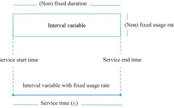
Vansteenwegen et al. [16] and Labadie et al. [1] provide integer programming models for TOPTW. In this section, we introduce a CP model for TOPTW. We utilize (time) interval variables that are capable of expressing several critical decisions such as start time, end time, duration and usage rate under one variable ([44], [45]). Interval variables are useful in order to represent complex scheduling and routing activities especially when they are optional (i.e. a task may or may not be processed, a customer may or may not be visited, etc.). Laborie and Rogerie [45] mention several advantages of interval variables. One is that the optionality is already modeled in the definition of the interval variable and there is no need for additional constraints in order to enforce this binary relationship, as the traditional integer decision variables require in scheduling problem formulations. As an example, if an optional interval variable is not present in the final solution, it is interpreted as its domain is empty and thus not considered in the final solution. However, in case of its presence in the final solution, we know that its domain contains a single value which is defined by its start and end time. Finally, its final status (absence or presence) can be queried by usingpresenceOf(Interval Variable)in the problem formulation.

(7)

In this application, the domains are the possible time periods when a location visit starts and ends. The duration of the visit is ﬁxed and equal to the diﬀerence between the visit redend time and start time.

Figure 1 and the list below explain other features of interval variables used in this application.

• Start and end time represents redservice start and end time of a visit, respectively. redRecall

that start time is not necessarily the time the vehicle arrives to a location, as the vehicle may need to wait until the time window begins.

• Only one vehicle is needed to initiate and terminate a visit. Therefore, usage rate is equal to

one. From this point forward, we represent an interval variable as a continuous line identiﬁed by the service start and end times.

Through the use of interval variables, we are able to dramatically reduce the number of decision variables and constraints needed to formulate the TOPTW model so that a model for even larger benchmark instances can be created without memory problems.

Interval variable

Service start time Service end time

(Non) fixed duration

(Non) fixed usage rate

Service time (si)

Interval variable with fixed usage rate

Figure 1: Interval variable attributes

We create an extra node n+ 1 (dummy depot) and add it to the node set N in order to model

vehicles returning to the depot. Also, we set t_i,n₊₁ =t_i,₀ for alli∈ N,e_n₊₁ =e₀ and b_n₊₁=b₀. The

following interval variables are then created with the appropriate service times:

• xiv, optional interval variable representing visiting node i∈ N, i= 0, i=n+ 1 using vehicle v

and with a service time ofs_i.

• yi, interval variable associated with i ∈ N. Interval variables of the depot, y0 and yn+1, are

mandatory (must be present in the solution) whereas interval variable y_i is optional for each

(8)

• Zi ={xi1, xi2, . . . , xiv, . . . , xim}, set of interval variables representing possible vehicles on which node i∈ N, i6= 0, i6=n+ 1 can be visited.

• Qv ={x1v, x2v, . . . , xiv, . . . , xnv}, set of interval variables representing possible nodesi∈ N that can be visited by vehiclesv∈ V. This set is also calledinterval sequence variableforv∈ V since it is used to evaluate the feasibility of a sequence for a vehicle.

We note that the time interval variable and its optionality feature as well as several global con-straints (Alternative, N oOverlap, P ulse etc.) used in this study are extracted from IBM’s CP Op-timizer. Due to the lack of standardization in defining variables and global constraints in the CP community, it may not be possible to run the exact same model in another solver such as OR Tools and Gecode because these features might be referred to using different names. CP Optimizer’s

Alternative(a0,{a1, . . . , an}) global constraint allows an exclusive alternative between interval vari-ables {a1, . . . , an} [45]. This constraint ensures that exactly one of the interval variables from the arbitrarily defined set {a1, . . . , an} will be executed if the arbitrarily defined interval variable a0 is executed. Moreover, a0 will start and end together with the one chosen from set {a1, . . . , an}. How-ever, a0 is not executed if none of the interval variables from {a1, . . . , an} are executed. This feature is utilized to assign visits to vehicles.

Laborie et al. [46] define T ransitionDistance(.) as a function that records minimal delays be-tween two successive non overlapping interval variables. This function is used as an input for an-other global constraint called N oOverlap({a₁, . . . , an}, T ransitionDistance(.)) that defines a chain of non-overlapping interval decision variables with minimal time between every two successive inter-val variables in the set {a1, . . . , an}. In this application, T ransitionDistance(.) is defined as a two dimensional array that stores the time between each location pair. Thus, the N oOverlap constraint assures that if a location is visited by a vehicle, the time for the next location visit must occur after the necessary travel time elapses and the same vehicle cannot visit more than one location at any given time (or travel to more than one location). Moreover, Laborie et al. [46] also present another global constraint called Cumulative that keeps track of the cumulative usage level of the resource by the activities (in terms of interval variables) over time. Laborie et al. [46] and IBM [44] present numerous elementary cumulative functions in order to describe the impact of individual interval variables over time. For instance, P ulseis used to model cumulative usage andStepis to describe resource produc-tion/consumption. In this application, the Cumulativeconstraint and its P ulsefunction are used to limit the total number of vehicles in use at any time to be less than or equal to the fleet size.

(9)

Given the interval variables and global constraints defined above, CP-TOPTW is as follows. maximize X i∈N piyi subject to (CP-TOPTW) Alternative(yi, Zi) i∈ N, i6= 0, i6=n+ 1 (1) Cumulative({y₀, y1, . . . , yn+1},1, m) (2) yi.StartM in=bi i∈ N (3) yi.StartM ax=ei i∈ N (4) N oOverlap(Qv, T ransitionDistance(tij|i∈N, j ∈N)) v∈ V (5) Qv.F irst(y0) v∈ V (6) Qv.Last(yn+1) v∈ V (7)

The objective function of CP-TOPTW seeks to maximize the total profit. Constraints (1) assure that each location except the depot (i = 0, n+ 1) is visited by at most one vehicle. This is made possible since the global Alternative constraint restricts only one of the Zi to be in the solution if

yi presents in the solution. Cumulative global constraints (2) are employed to model the usage of each vehicle v ∈ V during visits. They ensure the total number of busy vehicles at any time cannot exceed the number of available vehicles m. The vehicle usage over time is computed with the help of elementary sub-functionP ulse(yi). It increases and decreases the cumulative usage of busy vehicles by one at the start and end of interval variable yj, respectively. Note that if the vehicles were dissimilar, we would define a specific Cumulativeconstraint and P ulsefunction for eachv∈ V.

The time window for each location is defined by constraints (3) and (4). The former set the minimum start time (bi) and the latter set the maximum start time (ei) of a location. NoOverlap constraints (5) assure that the interval variables in Qv represent the possible visits of vehicle v ∈ V in order of the non-overlapping intervals. Furthermore, with the help of T ransitionDistance(tij),

N oOverlap global constraints create a minimal travel time (tij) between the end of interval variable

xiv and the start of interval variable xjv for the pair of consecutive visit locations i and j. Finally, constraints (6) and (7) make the depot the first and the last location to be visited by each vehicle

(10)

A very important advantage of CP-TOPTW compared to its ILP counterparts in Vansteenwegen et al. [16] and Labadie et al. [1] is that the number of constraints is no longer exponentially growing with the size of the input such as number of customers, vehicles and tour duration. The usage of interval variables replaces the time variables (arrival time, service start time etc.) since these decisions are in the domains of interval variables. Moreover, their sets (interval sequence variables) and Alternative

constraints are used to intelligently handle vehicle assignments to visits in such a way that a tour structure is maintained while subtours are prevented.

2.2 An illustrative example

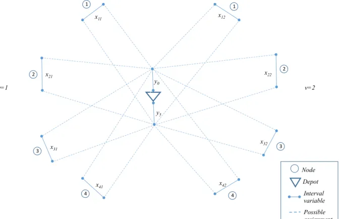
We illustrate the functionality of interval variables and constraints of (CP-TOPTW) over a simple TOPTW instance with four nodes (n = 4) and two vehicles (m = 2). Recall that each node i ∈ {1,2,3,4} can be visited by at most one vehicle v ∈ {1,2} in the TOPTW and this restriction is enforced by creating an optional interval variable for each possible assignment as shown in Figure 2. Thus, possible nodes that can be visited by vehicle v form an interval sequence variable Qv =

{x₁_v, x2v, x3v, x4v}. Similarly, possible vehicle assignment to a nodeiis represented by a set of interval variables Zi = {xi1, xi2}. The length of an interval variable represents the service time si required to visit node iand remains unchanged regardless of vehicle assignment decisions. As a consequence, assignment dependent service durations in case of dissimilar vehicles could also be modeled using the same scheme.

Tour start and end events are modeled as mandatory interval variables. Figure 2 shows that each tour must be initiated and ended by interval variables y0 and yn+1=5 with zero service time. This

restriction is enforced by making y0 and y5 as the first and last interval variables of interval sequence

variables Q1 andQ2 that stand for the tour of vehicle 1 and 2, respectively.

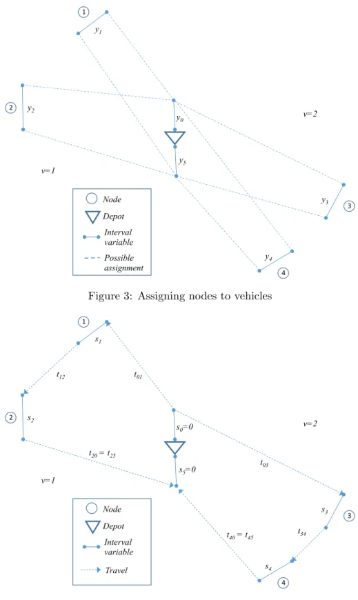
For the sake of simplicity, we assume that the first two nodes are assigned to the first vehicle and last two nodes are visited by the second vehicle as seen in Figure 3. TheAlternativeconstraint ensures that a node can only be visited by at most one vehicle (i.e. at most one of the interval variables in set

Zi can be in the solution). Furthermore, it requires optional interval variableyi fori= 1,2,3,4 to be present in the solution if any element ofZi is present. Recall that service time window restrictions are handled by explicitly specifying the minimum start and end times ofyinterval variables. The sequence in each tour (for eachv) is identified by theN oOverlapconstraint that takes interval sequence variable (Qv) and travel distances (tij) defined in the T ransitionDistance function as input parameters. It

(11)

5 1 y0 y5 x11 x21 x31 x41 x12 x22 x32 x42 v=1 v=2 Node Depot Interval variable Possible assignment 1" _1" ₁ 1 2" 1 2" 1 3" 3" 1 1 4" _4" ₁

Figure 2: Depot, nodes and interval variables

makes sure that a tour for vehiclevis formed in such a way that interval variables inQv do not overlap with each other during service and travel as illustrated in Figure 4. red For this particular example, customer 3 and 4 are assigned to the second vehicle and the optimal tour is formed as 0−3−4−0. This is indicated as y0 → y3 → y4 → y5 and s0 → s3 → s4 → s5 in terms of interval variables and

their visit durations, respectively. If the optimal tour was 0−4−3−0, this would be indicated as

y0 →y4→y3 →y5 by interval variables ands0→s4 →s3 →s5 by service times.

Finally, theCumulativeglobal constraint is utilized to capture vehicle usage for each assignment scheme. This constraint is redundant since all restrictions of the TOPTW are already handled by other global constraints. However, it tightens the CP formulation by reducing the domains of interval variables and makes the domain filtering algorithms more efficient. In coordination with other global variables, the Cumulativeconstraint assures that the total number of busy vehicles in use must be smaller than or equal tom= 2 at all times while itsP ulsefunction increases and decreases the number of busy vehicles by one at the beginning and end of each interval variable as demonstrated in Figure 5. A vehicle is labeled as busy only when it is serving a customer.

(12)

y0 y5 y1 y2 y3 y4 v=1 v=2 Node Depot Interval variable Possible assignment 1 1" 1 2" 1 3" 1 4"

Figure 3: Assigning nodes to vehicles

s0=0 s1 s2 s3 s4 v=1 v=2 Node Depot Interval variable Travel t01 t12 t20 = t25 t03 t34 t40 = t45 s5=0 1 1" 1 2" 1 3" 1 4"

Figure 4: Creating tours (sequences) by interval variables

2.3 Customized branching strategy

Propagation (domain filtering) algorithms filter out the domain of each interval decision variable into a single value in order to identify a feasible solution. If there is a variable left with multiple values in

(13)

v=2 v=1 # of bus y ve hi cl es s1 t01 t12 s2 t20 0 s4 t34 t40 t03 0 1 2 Time Time Vehicle s3 0

Figure 5: Reactions ofCumulativeconstraint (bottom) andP ulsefunction (bottom) to tours (top)

the domain after propagation algorithms, branching (value instantiation) takes place and the search continues. The most important factor in reaching a feasible solution within shorter computational time is to adopt an efficient branching strategy that exploits the benefits of problem structure(s) by selecting the best branching variable and value instantiation order. The CP Optimizer’s default search strategy works under the assumption that the current problem is infeasible or it is extremely hard to find a feasible solution [47]. This is referred to as the failure directed search (FDS) strategy. Thus, before a solution is found or infeasibility is reached, FDS explores the majority of the entire search space in order to prove infeasibility or optimality. However, we lack information regarding how the heuristics in the CP Optimizer’s library select the order of the interval variables to be fixed.

In addition to CP Optimizer’s default value instantiation order, we develop another customized method in which we first allow value instantiation on interval sequence variables, Qv. That is, we first let CP Optimizer fix the sequence of interval variables (visits) on interval sequence variables (vehicles). Of course, this requires deciding which interval variables (visits) are present in the solution (are visited) as enforced by constraints (1). Then, we let CP decide the right start and end times from the domains of interval variables. In the next section, we observe the performance of this proposed technique over the default branching strategy that does not require an order in branching variable selection. This prioritization is made possible by CP Optimizer’s IloSearchP hase that allows the user to define the value instantiation order of the interval decision variables.

(14)

3 Computational Results

This section presents the computational study and its results. We first describe TOPTW benchmark instances. Next, we present and discuss computational results.

3.1 Experiments

The performance of the model was compared with state-of-the-art algorithms on the TOPTW test instances taken from http://www.mech.kuleuven.be/en/cib/op. The instances we consider from Righ-ini and Salani [21], Montemanni and Gambardella [12], and Vansteenwegen et al.[16]. The TOPTW instances from Montemanni and Gambardella [12] were created by increasing the number of vehicles in the OPTW instances from Righini and redSalani [21]. Instances with 2, 3 and 4 vehicles are available. Among these instances, 56 were converted from the Solomon [13] VRPTW instances (sets c* 100, r* 100, rc* 100, c* 200, r* 200 and rc* 200). All of these instances have 100 nodes and we refer to them as the Solomon instances. Additionally, 20 of the test instances are converted from the Cordeau et al. [14] VRPTW instances (sets pr01-pr20) and contain between 48 and 288 nodes. We refer to these as the Cordeau instances. The instances provided in Vansteenwegen et al. [16] are also based on the Solomon and Cordeau instances. We refer to these as new instances, as in other TOPTW literature (e.g., [1, 16, 17]). For each of the new instances, the optimal solution is the sum of all profits; visiting all vertices is possible.

Distances between visit locations are rounded down to the first decimal for the Solomon instances and to the second decimal for the Cordeau instances (see [1, 11, 12, 14, 16, 17, 18, 21]). Because fractional distances create infinite domain ranges, it is impossible for propagation algorithms to identify a feasible solution in finite time. Thus, we multiply the rounded down distances in Solomon and Cordeau instances by 10 and 100, respectively. In order to have all parameters on the same scale, we also use these multipliers for service time and time window start and end times. Although this adjustment allows propagation algorithms to filter decision variable domains, it increases the number of possible values in the domains.

The model was implemented in C++, using IBM ILOG CP Optimizer 12.6 for its solution. All experiments were run on an Intel Xeon X7350 equipped with 2.93 GHz and 16 GB of RAM. The model terminates with the best feasible solution at the end of 30 minutes runtime unless an optimal solution is found earlier. redExcept where explicitly noted, all computational results reported in this study are obtained by using default branching rules with CP-TOPTW and a RestartFailLimit parameter

(15)

value of 100. This setting enforces that the CP search must be restarted once 100 failed branching attempts are reached. We tried several values for RestartLimit during our preliminary investigation phase. Based on our observations, large (>100) and small (<50) values for this search parameter increases the computational time dramatically. The values we tested between 50 and 100 did not result in any improvement on average % gap and number of best known solutions. On the other hand,RestartLimit=100 gave us better results in terms of these performance measures than the model with RestartLimit=50. Therefore, we use it for all problem instances except for two that resulted in significant improvements. The exceptions are pr01 with 1 vehicle and r202 with 2 vehicles, the results of which are obtained by setting RestartLimitto 50.

3.2 Results

The results of the proposed CP model for TOPTW are compared to the following state-of-the-art methods.

• ABC: artificial bee colony algorithm [19]

• I3CH: iterative three-component heuristic [18]

• GVNS: granular variable neighborhood search based on linear programming [1]

• SSA: slow version of the simulated annealing heuristic [17]

• VNS: variable neighbor search approach [11]

• ILS: iterated local search algorithm red [16]

• ACS: ant-colony system [12]

For each problem instance, we report CP results and existing results from the literature. Best-known results for the TOPTW benchmark instances presented in this study are taken from Hu and Lim [18] and Tae and Kim [20]. For ABC, I3CH, GVNS and ACS, the average objective value over 5 replicates is presented, as reported in the papers associated with those approaches. For VNS, the average objective value over 10 replicates for each instance is reported. For CP, no replications are required, so the results reported represent only a single objective value for each test instance.

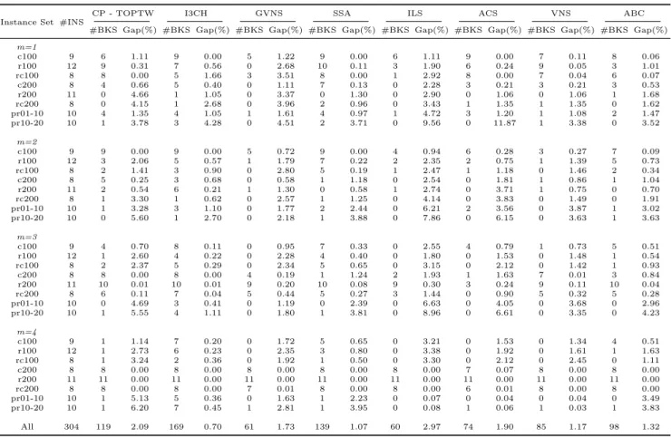
Table 1 summarizes the results for the Solomon and Cordeau instances. The number of vehiclesm

varies from 1 to 4. The #INS column shows the number of test instances in a set. The Gap(%) column for each algorithm reports the average percentage gap between solutions produced by the algorithm and the best-known solutions. The number of best-known solutions found by each algorithm is given in

(16)

while I3CH offers the best performance on this metric with an average gap of 0.70%. CP-TOPTW obtains best-known solutions for 119 out of 304 instances whereas GVNS, ILS, ACS, VNS, and ABC can only find the best-known solutions for 61, 60, 74, 85 and 95 instances, respectively. However, I3CH and SSA find more best-known solutions than CP-TOPTW does.

There are 89 instances for which CP-TOPTW was able to prove the optimality of the solution obtained. Table 2 provides information regarding these instances. For each instance, the optimal solution value is given, along with the time required by CP-TOPTW to return the solution and prove its optimality. The average computation time of CP-TOPTW for the set of instances reported in Table 2 is only 121 seconds. Bold text is used in the table to indicate optimality results for two instances which were previously unknown in the literature. The objective values for instance pr01 with 1 vehicle and instance pr11 with 4 vehicles were known previously but their optimality was not. For these two new optimality results, the default branching strategy was used. The default RestartFailLimit

parameter value of 100 was used for pr11 with 4 vehicles, while a value of 50 was used for pr01 with 1 vehicle. redCP-TOPTW discovers one new best-known solution. It is for instance r202 with 2 vehicles, and the objective value of the new solution is 1348. The solution is obtained using a customized branching rule and aRestartFailLimitparameter value of 50. CP-TOPTW improves upon the previously best-known solution for r202 by 0.07%.

Detailed results of all algorithms for the Solomon instances are given in Tables 3-6 for 1 through 4 vehicles, respectively. The first column provides the instance name and the second gives the best-known solution value, BKS. The additional columns provide the objective value (Profit) and percent gap to BKS for each instance and algorithm pair. Italicized text in the Profit column for CP-TOPTW indicates the solution was obtained using customized branching, while regular font indicates the solu-tion was obtained using default branching. CP-TOPTW usually achieves a better average percentage gap than GVNS and ILS over all of these instances. I3CH, SSA and ABC are competitive in terms of finding the best-known solution for most of these instances. Although the CP-TOPTW has slightly worse average optimality gap than I3CH, it is able to find better profit values for some of these instances than I3CH, SSA and ABC.

The solution values of the Cordeau instances are given in Tables 7-10. As seen in Table 7, CP outperforms I3CH for Cordeau instances (sets pr01-pr20) when m=1 with an average gap of 1.35% and 3.78%. In contrast, the performance of CP on the Cordeau instances is not as competitive as I3CH when m=2,3, and 4 (see Tables 8-10). CP-TOPTW usually achieves a better average percentage

(17)

Table 1: Comparison of CP-TOPTW to state-of-the-art algorithms on Solomon and Cordeau TOPTW instances

Instance Set #INS

CP - TOPTW I3CH GVNS SSA ILS ACS VNS ABC

#BKS Gap(%) #BKS Gap(%) #BKS Gap(%) #BKS Gap(%) #BKS Gap(%) #BKS Gap(%) #BKS Gap(%) #BKS Gap(%)

m=1 c100 9 6 1.11 9 0.00 5 1.22 9 0.00 6 1.11 9 0.00 7 0.11 8 0.06 r100 12 9 0.31 7 0.56 0 2.68 10 0.11 3 1.90 6 0.24 9 0.05 3 1.01 rc100 8 8 0.00 5 1.66 3 3.51 8 0.00 1 2.92 8 0.00 7 0.04 6 0.07 c200 8 4 0.66 5 0.40 0 1.11 7 0.13 0 2.28 3 0.21 3 0.21 3 0.53 r200 11 0 4.66 1 1.05 0 3.37 0 1.30 0 2.90 0 1.06 0 1.06 1 1.68 rc200 8 0 4.15 1 2.68 0 3.96 2 0.96 0 3.43 1 1.35 1 1.35 0 1.62 pr01-10 10 4 1.35 4 1.05 1 1.61 4 0.97 1 4.72 3 1.20 1 1.08 2 1.47 pr10-20 10 1 3.78 3 4.28 0 4.51 2 3.71 0 9.56 0 11.87 1 3.38 0 3.52 m=2 c100 9 9 0.00 9 0.00 5 0.72 9 0.00 4 0.94 6 0.28 3 0.27 7 0.09 r100 12 3 2.06 5 0.57 1 1.79 7 0.22 2 2.35 2 0.75 1 1.39 5 0.73 rc100 8 2 1.41 3 0.90 0 2.80 5 0.19 1 2.47 1 1.18 0 1.46 2 0.34 c200 8 5 0.25 3 0.68 0 0.58 1 1.18 0 2.54 0 1.81 1 0.86 1 1.04 r200 11 2 0.54 6 0.21 1 1.30 0 0.58 1 2.74 0 3.71 1 0.75 0 0.70 rc200 8 1 3.30 1 0.62 0 2.57 1 1.25 0 4.14 0 3.83 0 1.49 0 1.91 pr01-10 10 1 3.28 3 1.10 0 1.77 2 2.44 0 6.21 2 3.56 0 3.87 1 3.02 pr10-20 10 0 5.60 1 2.70 0 2.18 1 3.88 0 7.86 0 6.15 0 3.63 1 3.63 m=3 c100 9 4 0.70 8 0.11 0 0.95 7 0.33 0 2.55 4 0.79 1 0.73 5 0.51 r100 12 1 2.60 4 0.22 0 2.28 4 0.40 0 1.80 0 1.53 0 1.48 1 0.54 rc100 8 2 2.37 5 0.29 0 2.34 5 0.65 0 3.15 0 2.12 0 1.42 1 0.93 c200 8 8 0.00 8 0.00 4 0.19 1 1.24 2 1.93 1 1.63 7 0.01 3 0.84 r200 11 10 0.01 10 0.01 9 0.20 10 0.08 9 0.30 3 0.24 9 0.11 10 0.04 rc200 8 6 0.11 7 0.04 5 0.44 5 0.27 3 1.44 0 0.90 5 0.32 5 0.28 pr01-10 10 0 4.69 3 0.41 0 1.19 0 2.39 0 6.63 0 4.05 0 3.68 0 2.96 pr10-20 10 1 5.55 4 1.11 0 1.80 1 3.81 0 8.96 0 6.61 0 3.35 0 4.23 m=4 c100 9 1 1.14 7 0.20 0 1.72 5 0.65 0 3.21 0 1.53 0 1.34 4 0.51 r100 12 1 2.73 6 0.23 0 2.35 3 0.80 0 3.38 0 1.92 0 1.61 1 1.63 rc100 8 1 3.24 2 0.36 0 1.92 1 0.50 0 3.30 0 2.12 0 2.45 0 1.11 c200 8 8 0.00 8 0.00 8 0.00 8 0.00 8 0.00 7 0.07 8 0.00 8 0.00 r200 11 11 0.00 11 0.00 11 0.00 11 0.00 11 0.00 11 0.00 11 0.00 11 0.00 rc200 8 8 0.00 8 0.00 7 0.01 8 0.00 8 0.00 6 0.01 8 0.00 8 0.00 pr01-10 10 1 5.13 5 0.36 0 1.63 1 2.23 0 0.07 0 0.04 0 0.04 0 3.49 pr10-20 10 1 6.20 7 0.45 1 2.81 1 3.95 0 0.08 1 0.06 1 0.03 1 3.83 All 304 119 2.09 169 0.70 61 1.73 139 1.07 60 2.97 74 1.90 85 1.17 98 1.32

(18)

Table 2: Optimal solution values for Solomon and Cordeau TOPTW instances proved by CP-TOPTW

Instance Name m Optimal Solution Time (s) Instance Name m Optimal Solution Time (s) Instance Name m Optimal Solution Time (s)

c101 1 320 1173.0 rc204 3 1724 4.7 rc207 4 1724 1.5 r101 1 198 23.9 rc206 3 1724 4.5 rc208 4 1724 1.0 r105 1 247 155.3 rc207 3 1724 11.0 c101 10 1810 2.2 rc101 1 219 50.7 rc208 3 1724 0.7 c102 10 1810 4.7 rc102 1 266 418.6 c201 4 1810 1.1 c103 10 1810 26.3 rc105 1 244 184.1 c202 4 1810 1.4 c104 10 1810 7.1 rc106 1 252 507.6 c203 4 1810 1.5 c105 10 1810 553.7 r208 2 1458 117.6 c204 4 1810 1.2 c106 10 1810 6.5 r208 2 1458 202.2 c205 4 1810 1.1 c107 10 1810 3.9 c201 3 1810 1.0 c206 4 1810 1.2 c108 10 1810 5.6 c202 3 1810 3.6 c207 4 1810 1.0 c109 10 1810 2.6 c203 3 1810 14.1 c208 4 1810 2.0 r104 10 1724 218.3 c204 3 1810 461.3 r201 4 1458 1.6 r111 10 1458 1074.1 c205 3 1810 1.7 r202 4 1458 1.5 rc103 11 1724 218.5 c206 3 1810 5.1 r203 4 1458 1.4 rc107 11 1724 768.6 c207 3 1810 1.3 r204 4 1458 1.1 r106 12 1458 638.4 c208 3 1810 1.3 r205 4 1458 1.7 r103 13 1458 125.9 r202 3 1458 111.5 r206 4 1458 1.6 r105 14 1458 222.9 r203 3 1458 6.2 r207 4 1458 2.0 rc101 14 1724 454.9 r204 3 1458 1.7 r208 4 1458 1.0 r102 17 1458 9.5 r205 3 1458 2.5 r209 4 1458 0.9 r101 19 1458 6.4 r205 3 1458 3.0 r210 4 1458 1.9 pr01 1 308 459.3 r206 3 1458 1.2 r211 4 1458 1.9 pr01 4 657 1.1 r207 3 1458 1.4 rc201 4 1724 3.2 pr11 4 657 0.9 r208 3 1458 1.2 rc202 4 1724 2.4 pr05 15 3351 147.7 r209 3 1458 1.2 rc203 4 1724 2.3 pr06 18 3671 703.3 r210 3 1458 1.6 rc204 4 1724 1.8 pr08 10 2006 1011.1 r211 3 1458 1.2 rc205 4 1724 1.8 pr09 15 2736 80.8 rc202 3 1724 441.4 rc205 4 1724 2.7 pr10 20 3850 34.5 rc203 3 1724 15.9 rc206 4 1724 1.6

gap than ILS over all of these instances, except when m=4. It can be also observed that the average performance of CP on the Cordeau instances in terms of the average gap from the best-known solutions decreases when the number of vehicles increases. For example, the average gap of CP increases for instance sets pr01-pr10 from 1.35% to 3.28%, 4.69%, and 5.13% when the number of vehicles increases from 1 to 2, 3 and 4, respectively.

CP-TOPTW was also compared with state-of-the-art algorithms on the new instances. Recall it is known that the optimal solution for each of these instances is the sum of all possible profits. Table 11 compares the algorithms on these instances. In this table, the #INS column reports the number of test instances in the corresponding sets, the #OPT lists the number of optimal solutions and the Gap (%) column gives the average percentage gap from the optimal solution. On average, the gap between CP-TOPTW and the optimal solution is only 0.24%. For 48 out of 66 instances, CP-TOPTW is able to find the optimal solution whereas I3CH finds 55 optimal solutions with 0.14% optimality gap on average. For rc200 dataset instances, our model finds optimal solutions for allinstances while the state-of-the-art algorithms included in the comparison obtain optimal results in 7 out of 8 instances. It can be concluded that CP-TOPTW outperforms GVNS, SSA, ILS and ABC in terms of the percentage gap

(19)

and the number of optimal solutions found while the performance of I3CH is slightly better than CP-TOPTW. However, a primary advantage of CP-TOPTW over I3CH or any other heuristic algorithm is that CP-TOPTW states whether the obtained solution is optimal whereas the heuristic algorithms cannot.

Finally, detailed results obtained by CP-TOPTW for the new instances with known optimal so-lutions are provided in Tables 12 and 13. Based on these results, CP-TOPTW performs better on Solomon instances than Cordeau instances in terms of solution quality. The average gaps of Cordeau and Solomon test instances are 0.89% and 0.24%, respectively. Furthermore, the solution quality of CP-TOPTW is better than that of GVNS, SSA, ILS, and ABC on Cordeau instances. It can also be seen that the solution quality of both CP-TOPTW and I3CH are very close to optimal solutions for Solomon instances although the average gap of I3CH is smaller than that of CP-TOPTW.

(20)

Table 3: Detailed results for Solomon instances with m=1

Instance BKS

CP I3CH GVNS SSA ILS ABC

Instance BKS

Profit Gap(%) Profit Gap(%) Profit Gap(%) Profit Gap(%) Profit Gap(%) Profit Gap(%) Profit Gap(%) Profit Gap(%) Profit Gap(%) Profit Gap(%) Profit Gap(%) Profit Gap(%)

c101 320 320 0.00 320 0.00 320 0.00 320 0.00 320 0.00 320 0.00 c201 870 870 0.00 870 0.00 850 2.30 870 0.00 840 3.45 870 0.00 c102 360 360 0.00 360 0.00 360 0.00 360 0.00 360 0.00 360 0.00 c202 930 930 0.00 930 0.00 916 1.51 930 0.00 910 2.15 930 0.00 c103 400 390 2.50 400 0.00 396 1.00 400 0.00 390 2.50 398 0.50 c203 960 960 0.00 960 0.00 956 0.42 960 0.00 940 2.08 958 0.21 c104 420 400 4.76 420 0.00 410 2.38 420 0.00 400 4.76 420 0.00 c204 980 960 2.04 970 1.02 966 1.43 970 1.02 950 3.06 966 1.43 c105 340 340 0.00 340 0.00 340 0.00 340 0.00 340 0.00 340 0.00 c205 910 910 0.00 900 1.10 898 1.32 910 0.00 900 1.10 900 1.10 c106 340 340 0.00 340 0.00 340 0.00 340 0.00 340 0.00 340 0.00 c206 930 920 1.08 920 1.08 922 0.86 930 0.00 910 2.15 928 0.22 c107 370 360 2.70 370 0.00 358 3.24 370 0.00 360 2.70 370 0.00 c207 930 920 1.08 930 0.00 928 0.22 930 0.00 910 2.15 918 1.29 c108 370 370 0.00 370 0.00 354 4.32 370 0.00 370 0.00 370 0.00 c208 950 940 1.05 950 0.00 942 0.84 950 0.00 930 2.11 950 0.00 c109 380 380 0.00 380 0.00 380 0.00 380 0.00 380 0.00 380 0.00 r101 198 198 0.00 198 0.00 197 0.51 198 0.00 182 8.08 190 4.04 r201 797 792 0.63 789 1.00 775.6 2.69 794 0.38 788 1.13 787 1.25 r102 286 286 0.00 286 0.00 274.8 3.92 286 0.00 286 0.00 281.6 1.54 r202 930 872 6.24 930 0.00 881.4 5.23 914 1.72 880 5.38 895.8 3.68 r103 293 293 0.00 293 0.00 286 2.39 293 0.00 286 2.39 292 0.34 r203 1021 962 5.78 1020 0.10 992.2 2.82 997 2.35 980 4.02 1009 1.18 r104 303 303 0.00 298 1.65 298.6 1.45 303 0.00 297 1.98 299.6 1.12 r204 1086 1048 3.50 1073 1.20 1074 1.10 1058 2.58 1073 1.20 1070.4 1.44 r105 247 247 0.00 247 0.00 230.6 6.64 247 0.00 247 0.00 242.6 1.78 r205 953 892 6.40 946 0.73 905.8 4.95 946 0.73 931 2.31 953 0.00 r106 293 293 0.00 293 0.00 280.4 4.30 293 0.00 293 0.00 289 1.37 r206 1029 953 7.39 1021 0.78 966.6 6.06 1020 0.87 996 3.21 1018 1.07 r107 299 297 0.67 297 0.67 287.2 3.95 297 0.67 288 3.68 299 0.00 r207 1072 1012 5.60 1050 2.05 1022 4.66 1069 0.28 1038 3.17 1060.8 1.04 r108 308 306 0.65 306 0.65 301.4 2.14 306 0.65 297 3.57 308 0.00 r208 1112 1078 3.06 1092 1.80 1084 2.52 1079 2.97 1069 3.87 1084.6 2.46 r109 277 277 0.00 277 0.00 276.4 0.22 277 0.00 276 0.36 277 0.00 r209 950 926 2.53 948 0.21 926 2.53 945 0.53 926 2.53 934.6 1.62 r110 284 284 0.00 284 0.00 279.2 1.69 284 0.00 281 1.06 282.2 0.63 r210 987 939 4.86 982 0.51 961.4 2.59 973 1.42 958 2.94 965.4 2.19 r111 297 297 0.00 295 0.67 290.6 2.15 297 0.00 295 0.67 294 1.01 r211 1046 991 5.26 1013 3.15 1026 1.91 1041 0.48 1023 2.20 1019 2.58 r112 298 291 2.35 289 3.02 289.6 2.82 298 0.00 295 1.01 297 0.34 rc101 219 219 0.00 219 0.00 219 0.00 219 0.00 219 0.00 219 0.00 rc201 795 785 1.26 795 0.00 784 1.38 795 0.00 780 1.89 784 1.38 rc102 266 266 0.00 266 0.00 246 7.52 266 0.00 259 2.63 266 0.00 rc202 936 905 3.31 924 1.28 890.6 4.85 930 0.64 882 5.77 926.8 0.98 rc103 266 266 0.00 266 0.00 253.2 4.81 266 0.00 265 0.38 266 0.00 rc203 1003 930 7.28 966 3.69 954.4 4.85 967 3.59 960 4.29 962.4 4.05 rc104 301 301 0.00 301 0.00 301 0.00 301 0.00 297 1.33 301 0.00 rc204 1140 1066 6.49 1093 4.12 1102 3.33 1140 0.00 1117 2.02 1109.2 2.70 rc105 244 244 0.00 244 0.00 227 6.97 244 0.00 221 9.43 244 0.00 rc205 859 812 5.47 847 1.40 843.8 1.77 854 0.58 840 2.21 852.3 0.78 rc106 252 252 0.00 250 0.79 252 0.00 252 0.00 239 5.16 251.4 0.24 rc206 895 874 2.35 863 3.58 866.6 3.17 885 1.12 860 3.91 890.2 0.54 rc107 277 277 0.00 274 1.08 261.2 5.70 277 0.00 274 1.08 276.2 0.29 rc207 983 952 3.15 957 2.64 911.4 7.28 977 0.61 926 5.80 977 0.61 rc108 298 298 0.00 264 11.41 288.8 3.09 298 0.00 288 3.36 298 0.00 rc208 1053 1012 3.89 1003 4.75 1000 5.03 1041 1.14 1037 1.52 1032.8 1.92 Avg 0.47 0.69 2.46 0.05 1.94 0.46 Avg 3.32 1.34 2.88 0.85 2.87 1.32 19

(21)

Instance BKS

c101 590 590 0.00 590 0.00 590 0.00 590 0.00 590 0.00 590 0.00 c201 1460 1460 0.00 1450 0.68 1450 0.68 1450 0.68 1400 4.11 1450 0.68 c102 660 660 0.00 660 0.00 648 1.82 660 0.00 650 1.52 660 0.00 c202 1470 1470 0.00 1470 0.00 1464 0.41 1460 0.68 1430 2.72 1458 0.82 c103 720 720 0.00 720 0.00 704 2.22 720 0.00 700 2.78 716 0.56 c203 1480 1470 0.68 1470 0.68 1464 1.08 1450 2.03 1430 3.38 1450 2.03 c104 760 760 0.00 760 0.00 746 1.84 760 0.00 750 1.32 758 0.26 c204 1480 1480 0.00 1480 0.00 1472 0.54 1450 2.03 1460 1.35 1450 2.03 c105 640 640 0.00 640 0.00 640 0.00 640 0.00 640 0.00 640 0.00 c205 1470 1470 0.00 1450 1.36 1466 0.27 1470 0.00 1450 1.36 1470 0.00 c106 620 620 0.00 620 0.00 620 0.00 620 0.00 620 0.00 620 0.00 c206 1480 1480 0.00 1480 0.00 1472 0.54 1460 1.35 1440 2.70 1470 0.68 c107 670 670 0.00 670 0.00 670 0.00 670 0.00 670 0.00 670 0.00 c207 1490 1480 0.67 1470 1.34 1484 0.40 1480 0.67 1450 2.68 1477 0.87 c108 680 680 0.00 680 0.00 680 0.00 680 0.00 670 1.47 680 0.00 c208 1490 1480 0.67 1470 1.34 1480 0.67 1460 2.01 1460 2.01 1472 1.21 c109 720 720 0.00 720 0.00 716 0.56 720 0.00 710 1.39 720 0.00 r101 349 349 0.00 349 0.00 349 0.00 349 0.00 330 5.44 342.8 1.78 r201 1254 1246 0.64 1254 0.00 1225.8 2.25 1242 0.96 1231 1.83 1231.2 1.82 r102 508 470 7.48 508 0.00 492.8 2.99 508 0.00 508 0.00 508 0.00 r202 1347 1348 -0.07 1344 0.22 1306.2 3.03 1334 0.97 1270 5.72 1341.6 0.40 r103 522 515 1.34 519 0.57 506.6 2.95 519 0.57 513 1.72 517.2 0.92 r203 1416 1413 0.21 1416 0.00 1392.6 1.65 1414 0.14 1377 2.75 1410 0.42 r104 552 537 2.72 549 0.54 539.2 2.32 548 0.72 539 2.36 549 0.54 r204 1458 1452 0.41 1458 0.00 1452.6 0.37 1447 0.75 1440 1.23 1453.4 0.32 r105 453 453 0.00 447 1.32 442.6 2.30 453 0.00 430 5.08 448 1.10 r205 1380 1371 0.65 1380 0.00 1351.6 2.06 1363 1.23 1338 3.04 1365.8 1.03 r106 529 529 0.00 529 0.00 524.4 0.87 529 0.00 529 0.00 529 0.00 r206 1440 1433 0.49 1427 0.90 1429.8 0.71 1430 0.69 1401 2.71 1426.8 0.92 r107 538 537 0.19 533 0.93 522.2 2.94 532 1.12 529 1.67 518.8 3.57 r207 1458 1443 1.03 1458 0.00 1449.8 0.56 1452 0.41 1428 2.06 1448.4 0.66 r108 560 558 0.36 550 1.79 545.6 2.57 558 0.36 549 1.96 556 0.71 r208 1458 1458 0.00 1458 0.00 1458 0.00 1457 0.07 1458 0.00 1457.8 0.01 r109 506 505 0.20 506 0.00 501.6 0.87 506 0.00 498 1.58 502.8 0.63 r209 1405 1391 1.00 1404 0.07 1389.6 1.10 1404 0.07 1345 4.27 1390.2 1.05 r110 525 500 4.76 525 0.00 523 0.38 525 0.00 515 1.90 525 0.00 r210 1423 1407 1.12 1415 0.56 1391 2.25 1414 0.63 1365 4.08 1414.2 0.62 r111 544 520 4.41 542 0.37 530.6 2.46 544 0.00 535 1.65 544 0.00 r211 1458 1451 0.48 1450 0.55 1452.6 0.37 1451 0.48 1422 2.47 1451.2 0.47 r112 544 526 3.31 534 1.84 536.6 1.36 542 0.37 515 5.33 544 0.00 rc101 427 427 0.00 427 0.00 420.6 1.50 427 0.00 427 0.00 425.8 0.28 rc201 1384 1310 5.35 1384 0.00 1359.6 1.76 1377 0.51 1305 5.71 1373.2 0.78 rc102 505 504 0.20 505 0.00 485.4 3.88 505 0.00 494 2.18 505 0.00 rc202 1509 1494 0.99 1500 0.60 1465 2.92 1499 0.66 1461 3.18 1472.6 2.41 rc103 524 505 3.63 519 0.95 502 4.20 523 0.19 519 0.95 523 0.19 rc203 1632 1534 6.00 1627 0.31 1561.6 4.31 1576 3.43 1573 3.62 1593.6 2.35 rc104 575 575 0.00 556 3.30 554.8 3.51 575 0.00 565 1.74 572.8 0.38 rc204 1716 1660 3.26 1704 0.70 1699.2 0.98 1674 2.45 1656 3.50 1682 1.98 rc105 480 465 3.13 480 0.00 456.8 4.83 480 0.00 459 4.38 475.2 1.00 rc205 1458 1458 0.00 1452 0.41 1396 4.25 1458 0.00 1381 5.28 1446 0.82 rc106 483 480 0.62 481 0.41 480.4 0.54 483 0.00 458 5.18 483 0.00 rc206 1546 1469 4.98 1525 1.36 1507.4 2.50 1528 1.16 1495 3.30 1503.8 2.73 rc107 534 524 1.87 529 0.94 524 1.87 529 0.94 515 3.56 531.4 0.49 rc207 1587 1547 2.52 1582 0.32 1546.6 2.55 1574 0.82 1531 3.53 1561.8 1.59 rc108 556 546 1.80 547 1.62 544.6 2.05 554 0.36 546 1.80 554 0.36 rc208 1691 1636 3.25 1669 1.30 1669.6 1.27 1675 0.95 1606 5.03 1647.4 2.58 Avg 1.24 0.50 1.75 0.16 1.96 0.44 Avg 1.27 0.47 1.46 0.96 3.10 1.16 20

(22)

Instance BKS

c101 810 810 0.00 810 0.00 808 0.25 810 0.00 790 2.47 810 0.00 c201 1810 1810 0.00 1810 0.00 1800 0.55 1800 0.55 1750 3.31 1808 0.11 c102 920 920 0.00 920 0.00 916 0.43 920 0.00 890 3.26 920 0.00 c202 1810 1810 0.00 1810 0.00 1806 0.22 1790 1.10 1750 3.31 1792 0.99 c103 990 970 2.02 990 0.00 964 2.63 980 1.01 960 3.03 976 1.41 c203 1810 1810 0.00 1810 0.00 1804 0.33 1770 2.21 1760 2.76 1766 2.43 c104 1030 1020 0.97 1030 0.00 1012 1.75 1010 1.94 1010 1.94 1008 2.14 c204 1810 1810 0.00 1810 0.00 1802 0.44 1750 3.31 1780 1.66 1758 2.87 c105 870 860 1.15 870 0.00 864 0.69 870 0.00 840 3.45 868 0.23 c205 1810 1810 0.00 1810 0.00 1810 0.00 1810 0.00 1770 2.21 1804 0.33 c106 870 870 0.00 870 0.00 866 0.46 870 0.00 840 3.45 870 0.00 c206 1810 1810 0.00 1810 0.00 1810 0.00 1780 1.66 1770 2.21 1810 0.00 c107 910 900 1.10 910 0.00 906 0.44 910 0.00 900 1.10 910 0.00 c207 1810 1810 0.00 1810 0.00 1810 0.00 1800 0.55 1810 0.00 1810 0.00 c108 920 920 0.00 920 0.00 914 0.65 920 0.00 900 2.17 920 0.00 c208 1810 1810 0.00 1810 0.00 1810 0.00 1800 0.55 1810 0.00 1810 0.00 c109 970 960 1.03 960 1.03 958 1.24 970 0.00 950 2.06 962 0.82 r101 484 484 0.00 481 0.62 477.4 1.36 484 0.00 481 0.62 477.2 1.40 r201 1441 1440 0.07 1439 0.14 1416.4 1.71 1429 0.83 1408 2.29 1434.8 0.43 r102 694 662 4.61 691 0.43 674.2 2.85 694 0.00 685 1.30 690.6 0.49 r202 1458 1458 0.00 1458 0.00 1450.2 0.53 1458 0.00 1443 1.03 1458 0.00 r103 747 716 4.15 740 0.94 724.4 3.03 736 1.47 720 3.61 746 0.13 r203 1458 1458 0.00 1458 0.00 1458 0.00 1458 0.00 1458 0.00 1458 0.00 r104 778 754 3.08 777 0.13 762 2.06 777 0.13 765 1.67 777 0.13 r204 1458 1458 0.00 1458 0.00 1458 0.00 1458 0.00 1458 0.00 1458 0.00 r105 620 615 0.81 619 0.16 612.4 1.23 619 0.16 609 1.77 619.3 0.11 r205 1458 1458 0.00 1458 0.00 1458 0.00 1458 0.00 1458 0.00 1458 0.00 r106 729 716 1.78 729 0.00 713.4 2.14 729 0.00 719 1.37 725.8 0.44 r206 1458 1458 0.00 1458 0.00 1458 0.00 1458 0.00 1458 0.00 1458 0.00 r107 760 739 2.76 759 0.13 755 0.66 759 0.13 747 1.71 760 0.00 r207 1458 1458 0.00 1458 0.00 1458 0.00 1458 0.00 1458 0.00 1458 0.00 r108 797 771 3.26 797 0.00 770.4 3.34 789 1.00 790 0.88 785.8 1.41 r208 1458 1458 0.00 1458 0.00 1458 0.00 1458 0.00 1458 0.00 1458 0.00 r109 710 691 2.68 710 0.00 699.6 1.46 702 1.13 699 1.55 704 0.85 r209 1458 1458 0.00 1458 0.00 1458 0.00 1458 0.00 1458 0.00 1458 0.00 r110 737 720 2.31 736 0.14 716.2 2.82 734 0.41 711 3.53 734 0.41 r210 1458 1458 0.00 1458 0.00 1458 0.00 1458 0.00 1458 0.00 1458 0.00 r111 774 756 2.33 773 0.13 749.4 3.18 771 0.39 764 1.29 771 0.39 r211 1458 1458 0.00 1458 0.00 1458 0.00 1458 0.00 1458 0.00 1458 0.00 r112 776 749 3.48 776 0.00 751 3.22 776 0.00 758 2.32 770.8 0.67 rc101 621 621 0.00 621 0.00 602.4 3.00 621 0.00 604 2.74 617.4 0.58 rc201 1698 1693 0.29 1693 0.29 1676 1.30 1681 1.00 1625 4.30 1681 1.00 rc102 714 703 1.54 714 0.00 692 3.08 710 0.56 698 2.24 710.3 0.52 rc202 1724 1724 0.00 1724 0.00 1702.8 1.23 1714 0.58 1686 2.20 1717.4 0.38 rc103 764 702 8.12 764 0.00 741.2 2.98 764 0.00 747 2.23 748.6 2.02 rc203 1724 1724 0.00 1724 0.00 1724 0.00 1724 0.00 1724 0.00 1724 0.00 rc104 835 835 0.00 834 0.12 826 1.08 814 2.51 822 1.56 828 0.84 rc204 1724 1724 0.00 1724 0.00 1724 0.00 1724 0.00 1724 0.00 1724 0.00 rc105 682 666 2.35 682 0.00 670.2 1.73 682 0.00 654 4.11 682 0.00 rc205 1719 1709 0.58 1719 0.00 1702.2 0.98 1709 0.58 1659 3.49 1704.8 0.83 rc106 706 693 1.84 706 0.00 692.6 1.90 706 0.00 678 3.97 696.4 1.36 rc206 1724 1724 0.00 1724 0.00 1724 0.00 1724 0.00 1708 0.93 1724 0.00 rc107 773 759 1.81 762 1.42 756.4 2.15 773 0.00 745 3.62 769.8 0.41 rc207 1724 1724 0.00 1724 0.00 1724 0.00 1724 0.00 1713 0.64 1724 0.00 rc108 795 769 3.27 789 0.75 773 2.77 778 2.14 757 4.78 781.2 1.74 rc208 1724 1724 0.00 1724 0.00 1724 0.00 1724 0.00 1724 0.00 1724 0.00 Avg 1.95 0.21 1.88 0.45 2.41 0.64 Avg 0.04 0.02 0.27 0.48 1.12 0.35 21

(23)

Instance BKS

c101 1020 1020 0.00 1020 0.00 1014 0.59 1020 0.00 1000 1.96 1020 0.00 c201 1810 1810 0.00 1810 0.00 1810 0.00 1810 0.00 1810 0.00 1810 0.00 c102 1150 1140 0.87 1150 0.00 1132 1.57 1150 0.00 1090 5.22 1150 0.00 c202 1810 1810 0.00 1810 0.00 1810 0.00 1810 0.00 1810 0.00 1810 0.00 c103 1210 1180 2.48 1210 0.00 1178 2.64 1190 1.65 1150 4.96 1208 0.17 c203 1810 1810 0.00 1810 0.00 1810 0.00 1810 0.00 1810 0.00 1810 0.00 c104 1260 1240 1.59 1260 0.00 1226 2.70 1230 2.38 1220 3.17 1240 1.59 c204 1810 1810 0.00 1810 0.00 1810 0.00 1810 0.00 1810 0.00 1810 0.00 c105 1070 1060 0.93 1060 0.93 1060 0.93 1060 0.93 1030 3.74 1060 0.93 c205 1810 1810 0.00 1810 0.00 1810 0.00 1810 0.00 1810 0.00 1810 0.00 c106 1080 1070 0.93 1080 0.00 1052 2.59 1080 0.00 1040 3.70 1080 0.00 c206 1810 1810 0.00 1810 0.00 1810 0.00 1810 0.00 1810 0.00 1810 0.00 c107 1120 1110 0.89 1120 0.00 1112 0.71 1120 0.00 1100 1.79 1120 0.00 c207 1810 1810 0.00 1810 0.00 1810 0.00 1810 0.00 1810 0.00 1810 0.00 c108 1140 1120 1.75 1130 0.88 1116 2.11 1130 0.88 1100 3.51 1126 1.23 c208 1810 1810 0.00 1810 0.00 1810 0.00 1810 0.00 1810 0.00 1810 0.00 c109 1190 1180 0.84 1190 0.00 1170 1.68 1190 0.00 1180 0.84 1182 0.67 r101 611 606 0.82 608 0.49 607 0.65 611 0.00 601 1.64 603.6 1.21 r201 1458 1458 0.00 1458 0.00 1458 0.00 1458 0.00 1458 0.00 1458 0.00 r102 843 843 0.00 837 0.71 814.6 3.37 843 0.00 807 4.27 828 1.78 r202 1458 1458 0.00 1458 0.00 1458 0.00 1458 0.00 1458 0.00 1458 0.00 r103 928 914 1.51 928 0.00 902 2.80 926 0.22 878 5.39 920.2 0.84 r203 1458 1458 0.00 1458 0.00 1458 0.00 1458 0.00 1458 0.00 1458 0.00 r104 975 951 2.46 969 0.62 939 3.69 964 1.13 941 3.49 961 1.44 r204 1458 1458 0.00 1458 0.00 1458 0.00 1458 0.00 1458 0.00 1458 0.00 r105 778 767 1.41 778 0.00 770.6 0.95 771 0.90 735 5.53 753.8 3.11 r205 1458 1458 0.00 1458 0.00 1458 0.00 1458 0.00 1458 0.00 1458 0.00 r106 906 868 4.19 906 0.00 878.2 3.07 905 0.11 870 3.97 897.6 0.93 r206 1458 1458 0.00 1458 0.00 1458 0.00 1458 0.00 1458 0.00 1458 0.00 r107 950 899 5.37 950 0.00 932.8 1.81 942 0.84 927 2.42 937.2 1.35 r207 1458 1458 0.00 1458 0.00 1458 0.00 1458 0.00 1458 0.00 1458 0.00 r108 995 964 3.12 994 0.10 958.6 3.66 977 1.81 982 1.31 967 2.81 r208 1458 1458 0.00 1458 0.00 1458 0.00 1458 0.00 1458 0.00 1458 0.00 r109 885 837 5.42 885 0.00 869.4 1.76 885 0.00 866 2.15 885 0.00 r209 1458 1458 0.00 1458 0.00 1458 0.00 1458 0.00 1458 0.00 1458 0.00 r110 915 898 1.86 915 0.00 893.2 2.38 893 2.40 870 4.92 889 2.84 r210 1458 1458 0.00 1458 0.00 1458 0.00 1458 0.00 1458 0.00 1458 0.00 r111 953 908 4.72 952 0.10 937.4 1.64 948 0.52 935 1.89 948 0.52 r211 1458 1458 0.00 1458 0.00 1458 0.00 1458 0.00 1458 0.00 1458 0.00 r112 974 956 1.85 967 0.72 950.4 2.42 958 1.64 939 3.59 948 2.67 rc101 811 811 0.00 808 0.37 797.6 1.65 808 0.37 794 2.10 802.6 1.04 rc201 1724 1724 0.00 1724 0.00 1723 0.06 1724 0.00 1724 0.00 1724 0.00 rc102 909 906 0.33 899 1.10 887 2.42 902 0.77 881 3.08 902 0.77 rc202 1724 1724 0.00 1724 0.00 1724 0.00 1724 0.00 1724 0.00 1724 0.00 rc103 975 896 8.10 974 0.10 948.4 2.73 970 0.51 947 2.87 950 2.56 rc203 1724 1724 0.00 1724 0.00 1724 0.00 1724 0.00 1724 0.00 1724 0.00 rc104 1065 1017 4.51 1064 0.09 1036 2.72 1059 0.56 1019 4.32 1059 0.56 rc204 1724 1724 0.00 1724 0.00 1724 0.00 1724 0.00 1724 0.00 1724 0.00 rc105 875 867 0.91 875 0.00 866 1.03 875 0.00 841 3.89 861.8 1.51 rc205 1724 1724 0.00 1724 0.00 1724 0.00 1724 0.00 1724 0.00 1724 0.00 rc106 909 826 9.13 909 0.00 896.2 1.41 901 0.88 874 3.85 897.4 1.28 rc206 1724 1724 0.00 1724 0.00 1724 0.00 1724 0.00 1724 0.00 1724 0.00 rc107 987 980 0.71 980 0.71 963 2.43 980 0.71 951 3.65 977.2 0.99 rc207 1724 1724 0.00 1724 0.00 1724 0.00 1724 0.00 1724 0.00 1724 0.00 rc108 1025 1002 2.24 1020 0.49 1015 0.98 1023 0.20 998 2.63 1023 0.20 rc208 1724 1724 0.00 1724 0.00 1724 0.00 1724 0.00 1724 0.00 1724 0.00 Avg 2.38 0.26 2.04 0.67 3.30 1.14 Avg 0.00 0.00 0.00 0.00 0.00 0.00 22

(24)

Table 7: Detailed results for Cordeau instances with m=1

Instance BKS

Profit Gap (%) Profit Gap (%) Profit Gap (%) Profit Gap (%) Profit Gap (%) Profit Gap (%) Profit Gap (%) Profit Gap (%) Profit Gap (%) Profit Gap (%) Profit Gap (%) Profit Gap (%)

pr01 308 308 0.00 307.2 0.26 305 0.97 305 0.97 304 1.30 307 0.32 pr11 353 351 0.57 329 6.80 353 0.00 351 0.57 330 6.52 350.6 0.68 pr02 404 404 0.00 403.6 0.10 394 2.48 404 0.00 385 4.70 391.2 3.17 pr12 442 440 0.45 435 1.58 433 2.04 430 2.71 431 2.49 432 2.26 pr03 394 388 1.52 388 1.52 394 0.00 394 0.00 384 2.54 394 0.00 pr13 466 458 1.72 452.4 2.92 466 0.00 452 3.00 450 3.43 458.1 1.70 pr04 489 475 2.86 475.4 2.78 489 0.00 489 0.00 447 8.59 486 0.61 pr14 567 543 4.23 540.6 4.66 521 8.11 540 4.76 482 14.99 560.1 1.22 pr05 595 591 0.67 578 2.86 594 0.17 589 1.01 576 3.19 586.8 1.38 pr15 707 649 8.20 656.6 7.13 707 0.00 666 5.80 638 9.76 666.4 5.74 pr06 590 586 0.68 584.2 0.98 590 0.00 575 2.54 538 8.81 573.6 2.78 pr16 674 588 12.76 643.4 4.54 619 8.16 616 8.61 559 17.06 613.4 8.99 pr07 298 288 3.36 297 0.34 298 0.00 298 0.00 291 2.35 298 0.00 pr17 362 362 0.00 345.6 4.53 360 0.55 362 0.00 346 4.42 359 0.83 pr08 463 463 0.00 463 0.00 454 1.94 462 0.22 463 0.00 462 0.22 pr18 539 535 0.74 530.8 1.52 497 7.79 539 0.00 479 11.13 535 0.74 pr09 493 493 0.00 482 2.23 490 0.61 482 2.23 461 6.49 481.8 2.27 pr19 562 543 3.38 507.8 9.64 538 4.27 531 5.52 499 11.21 541 3.74 pr10 594 568 4.38 564.4 4.98 568 4.38 578 2.69 539 9.26 570.4 3.97 pr20 667 629 5.70 655 1.80 588 11.84 626 6.15 570 14.54 604.8 9.33 Avg 1.35 1.61 1.05 0.97 4.72 1.47 Avg 3.78 4.51 4.28 3.71 9.56 3.52

Instance BKS

pr01 502 502 0.00 495 1.39 502 0.00 502 0.00 471 6.18 502 0.00 pr11 566 559 1.24 539.4 4.70 559 1.24 566 0.00 542 4.24 558.2 1.38 pr02 715 699 2.24 706.4 1.20 714 0.14 712 0.42 660 7.69 704.6 1.45 pr12 774 750 3.10 750.8 3.00 768 0.78 759 1.94 727 6.07 754.8 2.48 pr03 742 736 0.81 718.4 3.18 731 1.48 741 0.13 714 3.77 738.4 0.49 pr13 832 803 3.49 827 0.60 832 0.00 825 0.84 757 9.01 831 0.12 pr04 924 856 7.36 903.8 2.19 917 0.76 905 2.06 863 6.60 905 2.06 pr14 1017 955 6.10 999 1.77 978 3.83 922 9.34 925 9.05 939.8 7.59 pr05 1101 1036 5.90 1073.6 2.49 1101 0.00 1053 4.36 1011 8.17 1045 5.09 pr15 12191120 8.12 1210.4 0.71 1205 1.15 1155 5.25 1126 7.63 1145.4 6.04 pr06 1076 1014 5.76 1070.2 0.54 1040 3.35 1022 5.02 997 7.34 1009.8 6.15 pr16 1231 1093 11.21 1217.8 1.07 1124 8.69 1094 11.13 1110 9.83 1106.4 10.12 pr07 566 561 0.88 557.8 1.45 566 0.00 566 0.00 552 2.47 559.2 1.20 pr17 652 628 3.68 626 3.99 639 1.99 643 1.38 624 4.29 652 0.00 pr08 834 810 2.88 824.4 1.15 824 1.20 822 1.44 796 4.56 806.6 3.29 pr18 938 910 2.99 914.4 2.52 937 0.11 929 0.96 877 6.50 929 0.96 pr09 909 887 2.42 883.4 2.82 878 3.41 854 6.05 867 4.62 859.2 5.48 pr19 1034 967 6.48 1004.4 2.86 1003 3.00 1017 1.64 955 7.64 1004.2 2.88 pr10 1124 1073 4.54 1109 1.33 1117 0.62 1069 4.89 1004 10.68 1067.4 5.04 pr20 1232 1114 9.58 1224.4 0.62 1155 6.25 1154 6.33 1056 14.29 1173.3 4.76 Avg 3.28 1.77 1.10 2.44 6.21 3.02 Avg 5.60 2.18 2.70 3.88 7.86 3.63 23

(25)

Instance BKS

pr01 622 611 1.77 608.4 2.19 622 0.00 614 1.29 598 3.86 617.4 0.74 pr11 654 654 0.00 647 1.07 654 0.00 654 0.00 632 3.36 652.2 0.28 pr02 942 925 1.80 937.8 0.45 936 0.64 939 0.32 899 4.56 930.9 1.18 pr12 1002 971 3.09 975.2 2.67 997 0.50 967 3.49 902 9.98 966 3.59 pr03 1010 998 1.19 997.4 1.25 1010 0.00 989 2.08 946 6.34 985.4 2.44 pr13 1145 1080 5.68 1102.2 3.74 1145 0.00 1139 0.52 1046 8.65 1111 2.97 pr04 1294 1197 7.50 1279.6 1.11 1286 0.62 1253 3.17 1195 7.65 1256 2.94 pr14 1372 1299 5.32 1357.4 1.06 1315 4.15 1289 6.05 1197 12.76 1279.4 6.75 pr05 14821423 3.98 1464 1.21 1481 0.07 1431 3.44 1356 8.50 1429.8 3.52 pr15 1654 1508 8.83 1594.2 3.62 1654 0.00 1550 6.29 1488 10.04 1588.4 3.97 pr06 1514 1373 9.31 1499.4 0.96 1501 0.86 1469 2.97 1376 9.11 1449 4.29 pr16 1668 1521 8.81 1654.6 0.80 1609 3.54 1530 8.27 1516 9.11 1521.2 8.80 pr07 744 737 0.94 736.6 0.99 738 0.81 742 0.27 713 4.17 738.2 0.78 pr17 841 837 0.48 822.4 2.21 841 0.00 838 0.36 808 3.92 826.6 1.71 pr08 11391106 2.90 1122.6 1.44 1139 0.00 1131 0.70 1082 5.00 1130.2 0.77 pr18 1281 1248 2.58 1270.8 0.80 1276 0.39 1262 1.48 1165 9.06 1241.2 3.11 pr09 12821171 8.66 1260.6 1.67 1272 0.78 1236 3.59 1144 10.76 1208.2 5.76 pr19 1417 1270 10.37 1393.6 1.65 1403 0.99 1329 6.21 1238 12.63 1340.2 5.42 pr10 1573 1434 8.84 1563.4 0.61 1567 0.38 1477 6.10 1473 6.36 1460.6 7.15 pr20 1684 1510 10.33 1677.6 0.38 1658 1.54 1593 5.40 1514 10.10 1587.8 5.71 Avg 4.69 1.19 0.41 2.39 6.63 2.96 Avg 5.55 1.80 1.11 3.81 8.96 4.23

Instance BKS

pr01 657 657 0.00 655.8 0.18 657 0.00 657 0.00 644 0.02 655.8 0.18 pr11 657 657 0.00 657 0.00 657 0.00 657 0.00 654 0.00 657 0.00 pr02 1079 1063 1.48 1064.2 1.37 1073 0.56 1069 0.93 1014 0.06 1053.6 2.35 pr12 11321090 3.71 1110.2 1.93 1120 1.06 1116 1.41 1041 0.08 1130.1 0.17 pr03 1232 1198 2.76 1209.6 1.82 1232 0.00 1201 2.52 1162 0.06 1198.4 2.73 pr13 1386 1279 7.72 1324.8 4.42 1386 0.00 1355 2.24 1263 0.09 1332.4 3.87 pr04 1585 1486 6.25 1525.8 3.74 1585 0.00 1535 3.15 1452 0.08 1525 3.79 pr14 1670 1553 7.01 1636.6 2.00 1651 1.14 1586 5.03 1528 0.09 1569.2 6.04 pr05 18381665 9.41 1811.4 1.45 1838 0.00 1759 4.30 1665 0.09 1755.4 4.49 pr15 20651881 8.91 1933.4 6.37 2065 0.00 1929 6.59 1818 0.12 1937.6 6.17 pr06 18601680 9.68 1840.4 1.05 1835 1.34 1839 1.13 1696 0.09 1763.6 5.18 pr16 20651828 11.48 2000 3.15 2017 2.32 1921 6.97 1889 0.09 1924 6.83 pr07 876 871 0.57 862.6 1.53 872 0.46 871 0.57 840 0.04 855.2 2.37 pr17 934 927 0.75 914.6 2.08 934 0.00 926 0.86 889 0.05 926.6 0.79 pr08 13821309 5.28 1358.2 1.72 1377 0.36 1358 1.74 1267 0.08 1336.8 3.27 pr18 15391496 2.79 1505.4 2.18 1539 0.00 1455 5.46 1352 0.12 1462.8 4.95 pr09 16191495 7.66 1595.4 1.46 1604 0.93 1565 3.34 1460 0.10 1532.8 5.32 pr19 17501543 11.83 1688.2 3.53 1750 0.00 1695 3.14 1560 0.11 1670.8 4.53 pr10 1943 1784 8.18 1903.6 2.03 1943 0.00 1853 4.63 1782 0.08 1842 5.20 pr20 2062 1902 7.76 2012 2.42 2062 0.00 1901 7.81 1846 0.10 1958.8 5.00 Avg 5.13 1.63 0.36 2.23 0.07 3.49 Avg 6.20 2.81 0.45 3.95 0.08 3.83 24

(26)

Table 11: Comparison of CP-TOPTW to the state-of-the-art methods on the new instances

Instance Set #INS

#BKS Gap(%) #BKS Gap(%) #BKS Gap(%) #BKS Gap(%) #BKS Gap(%) #BKS Gap(%)

c100 9 9 0.00 9 0.00 6 0.47 4 1.04 4 1.41 4 0.74 r100 12 6 0.46 8 0.07 0 1.55 3 0.42 0 1.93 2 0.43 rc100 8 4 0.17 8 0.00 0 1.29 1 0.35 0 2.06 1 0.45 c200 8 8 0.00 8 0.00 8 0.00 8 0.00 8 0.00 8 0.00 r200 11 8 0.17 9 0.07 7 0.17 7 0.16 7 0.62 8 0.09 rc200 8 8 0.00 7 0.04 6 0.16 7 0.07 5 0.47 6 2.03 pr01-10 10 5 0.89 6 0.78 3 1.25 4 1.04 1 2.32 4 1.05 All 66 48 0.24 55 0.14 30 0.70 34 0.44 25 1.26 33 0.68

Table 12: Detailed results for new Cordeau instances

Instance m OPT

Profit Gap (%) Profit Gap (%) Profit Gap (%) Profit Gap (%) Profit Gap (%) Profit Gap(%) pr01 3 657 622 5.33 619 5.78 608.4 7.40 614 6.54 608 7.46 617.4 6.03 pr02 6 1220 1198 1.80 1207 1.07 1198.8 1.74 1205 1.23 1180 3.28 1203.8 1.33 pr03 9 1788 1775 0.73 1781 0.39 1760.8 1.52 1758 1.68 1738 2.80 1764.6 1.31 pr04 12 2477 2468 0.36 2477 0.00 2467.4 0.39 2461 0.65 2428 1.98 2474.2 0.11 pr05 15 3351 3351 0.00 3351 0.00 3351 0.00 3351 0.00 3297 1.61 3351 0.00 pr06 18 3671 3671 0.00 3671 0.00 3670.6 0.01 3661 0.27 3650 0.57 3670.6 0.01 pr07 5 948 942 0.63 943 0.53 935 1.37 948 0.00 909 4.11 931.4 1.75 pr08 10 2006 2006 0.00 2006 0.00 2004.6 0.07 2006 0.00 1984 1.10 2006 0.00 pr09 15 2736 2736 0.00 2736 0.00 2736 0.00 2736 0.00 2729 0.26 2736 0.00 pr10 20 3850 3850 0.00 3850 0.00 3850 0.00 3847 0.08 3850 0.00 3850 0.00 Avg 0.89 0.78 1.25 1.04 2.32 1.05

(27)

Table 13: Detailed results for new Solomon instances

Instance m OPT

c101 10 1810 1810 0.00 1810 0.00 1754 3.09 1770 2.21 1720 4.97 1786 1.33 c201 4 1810 1810 0.00 1810 0.00 1810 0.00 1810 0.00 1810 0.00 1810 0.00 c102 10 1810 1810 0.00 1810 0.00 1794 0.88 1810 0.00 1790 1.10 1810 0.00 c202 4 1810 1810 0.00 1810 0.00 1810 0.00 1810 0.00 1810 0.00 1810 0.00 c103 10 1810 1810 0.00 1810 0.00 1810 0.00 1810 0.00 1810 0.00 1810 0.00 c203 4 1810 1810 0.00 1810 0.00 1810 0.00 1810 0.00 1810 0.00 1810 0.00 c104 10 1810 1810 0.00 1810 0.00 1810 0.00 1810 0.00 1810 0.00 1810 0.00 c204 4 1810 1810 0.00 1810 0.00 1810 0.00 1810 0.00 1810 0.00 1810 0.00 c105 10 1810 1810 0.00 1810 0.00 1810 0.00 1780 1.66 1770 2.21 1782 1.55 c205 4 1810 1810 0.00 1810 0.00 1810 0.00 1810 0.00 1810 0.00 1810 0.00 c106 10 1810 1810 0.00 1810 0.00 1806 0.22 1800 0.55 1750 3.31 1786 1.33 c206 4 1810 1810 0.00 1810 0.00 1810 0.00 1810 0.00 1810 0.00 1810 0.00 c107 10 1810 1810 0.00 1810 0.00 1810 0.00 1760 2.76 1790 1.10 1784 1.44 c207 4 1810 1810 0.00 1810 0.00 1810 0.00 1810 0.00 1810 0.00 1810 0.00 c108 10 1810 1810 0.00 1810 0.00 1810 0.00 1770 2.21 1810 0.00 1792 0.99 c208 4 1810 1810 0.00 1810 0.00 1810 0.00 1810 0.00 1810 0.00 1810 0.00 c109 10 1810 1810 0.00 1810 0.00 1810 0.00 1810 0.00 1810 0.00 1810 0.00 r101 19 1458 1458 0.00 1458 0.00 1432.2 1.77 1455 0.21 1441 1.17 1457.4 0.04 r201 4 1458 1458 0.00 1458 0.00 1458 0.00 1458 0.00 1458 0.00 1458 0.00 r102 17 1458 1458 0.00 1458 0.00 1441.2 1.15 1458 0.00 1450 0.55 1455.4 0.18 r202 3 1458 1458 0.00 1458 0.00 1450.2 0.53 1458 0.00 1443 1.03 1458 0.00 r103 13 1458 1458 0.00 1458 0.00 1446.6 0.78 1455 0.21 1450 0.55 1455 0.21 r203 3 1458 1458 0.00 1458 0.00 1458 0.00 1458 0.00 1458 0.00 1458 0.00 r104 9 14581439 1.30 1454 0.27 1418.2 2.73 1442 1.10 1402 3.84 1437.8 1.39 r204 2 1458 1452 0.41 1458 0.00 1452.6 0.37 1447 0.75 1440 1.23 1458 0.00 r105 14 1458 1458 0.00 1458 0.00 1441.6 1.12 1458 0.00 1435 1.58 1458 0.00 r205 3 1458 1458 0.00 1458 0.00 1458 0.00 1458 0.00 1458 0.00 1453.4 0.32 r106 12 1458 1458 0.00 1458 0.00 1437.6 1.40 1458 0.00 1441 1.17 1458 0.00 r206 3 1458 1458 0.00 1458 0.00 1458 0.00 1458 0.00 1458 0.00 1458 0.00 r107 10 1458 1444 0.96 1458 0.00 1435 1.58 1452 0.41 1431 1.85 1452 0.41 r207 2 14581443 1.03 1456 0.14 1449.8 0.56 1452 0.41 1428 2.06 1458 0.00 r108 9 14581446 0.82 1456 0.14 1441.8 1.11 1447 0.75 1430 1.92 1451.8 0.43 r208 2 1458 1458 0.00 1458 0.00 1458 0.00 1457 0.07 1458 0.00 1448.4 0.66 r109 11 1458 1455 0.21 1458 0.00 1433.4 1.69 1453 0.34 1432 1.78 1449.4 0.59 r209 3 1458 1458 0.00 1458 0.00 1458 0.00 1458 0.00 1458 0.00 1457.8 0.01 r110 10 1458 1443 1.03 1454 0.27 1433.4 1.69 1454 0.27 1419 2.67 1449 0.62 r210 3 1458 1458 0.00 1458 0.00 1458 0.00 1458 0.00 1458 0.00 1458 0.00 r111 10 1458 1458 0.00 1458 0.00 1430.2 1.91 1444 0.96 1410 3.29 1449.8 0.56 r211 2 1458 1451 0.48 1449 0.62 1452.6 0.37 1451 0.48 1422 2.47 1458 0.00 r112 9 1458 1440 1.23 1456 0.14 1434.4 1.62 1446 0.82 1418 2.74 1448 0.69 rc101 14 1724 1724 0.00 1724 0.00 1690.2 1.96 1712 0.70 1686 2.20 1713.6 0.60 rc201 4 1724 1724 0.00 1724 0.00 1724 0.00 1724 0.00 1724 0.00 1451.2 15.82 rc102 12 1724 1718 0.35 1724 0.00 1685 2.26 1718 0.35 1659 3.77 1705.2 1.09 rc202 3 1724 1724 0.00 1719 0.29 1702.8 1.23 1714 0.58 1686 2.20 1724 0.00 rc103 11 1724 1724 0.00 1724 0.00 1709 0.87 1724 0.00 1689 2.03 1721 0.17 rc203 3 1724 1724 0.00 1724 0.00 1724 0.00 1724 0.00 1724 0.00 1717.4 0.38 rc104 10 1724 1724 0.00 1724 0.00 1718 0.35 1719 0.29 1719 0.29 1723.4 0.03 rc204 3 1724 1724 0.00 1724 0.00 1724 0.00 1724 0.00 1724 0.00 1724 0.00 rc105 13 1724 1719 0.29 1724 0.00 1689.8 1.98 1716 0.46 1691 1.91 1716 0.46 rc205 4 1724 1724 0.00 1724 0.00 1723 0.06 1724 0.00 1724 0.00 1724 0.00 rc106 11 1724 1716 0.46 1724 0.00 1690.6 1.94 1714 0.58 1665 3.42 1706 1.04 rc206 3 1724 1724 0.00 1724 0.00 1724 0.00 1724 0.00 1708 0.93 1724 0.00 rc107 11 1724 1724 0.00 1724 0.00 1718.4 0.32 1722 0.12 1701 1.33 1724 0.00 rc207 3 1724 1724 0.00 1724 0.00 1724 0.00 1724 0.00 1713 0.64 1724 0.00 rc108 10 1724 1719 0.29 1724 0.00 1713 0.64 1719 0.29 1698 1.51 1720.6 0.20 rc208 3 1724 1724 0.00 1724 0.00 1724 0.00 1724 0.00 1724 0.00 1724 0.00 Avg 0.24 0.03 1.14 0.59 1.80 0.53 Avg 0.07 0.04 0.12 0.08 0.39 0.64 26