Commodity returns and their volatility in relation to speculation: A replication study 1

(1)

Commodity

returns

and

their

volatility

in

relation

to

speculation:

A

replication

study

1

Marco Haase

University of Basel, WWZ, Switzerland

Yvonne Seiler Zimmermann

Hochschule Luzern, IFZ, Switzerland

Heinz Zimmermann

University of Basel, WWZ, Switzerland

September 2015 – first version

Abstract

Granger causality (GC) tests are widely used when it comes to empirically address the dynamic rela‐

tionship between speculative activities and pricing on commodity markets. However, the sheer num‐

ber of studies and their heterogeneity makes it extremely difficult – if not impossible – to compare

their results and to derive meaningful conclusions. This is the main objective of this paper, which

analyzes a consistent dataset with a homogeneous estimation approach. We analyze futures returns

and volatilities of 28 commodities for three maturities, from January 2006 to March 2015, in relation

to three speculation proxies. Overall, we find a larger number of significant GC effects for volatilities

than for returns. The volatility effect is mostly negative, i.e. more speculation is followed by lower

volatilities. This is particularly true if the Working index used as speculation proxy. The majority of

destabilizing effects (positive relations) if any, is found in livestock. However, no such effects seem to

be present in typical agricultural commodities. Mixed evidence is found for softs. Apart from statisti‐

cal significance, the explained variance of returns and volatilities is below 8% and therefore economi‐

cally small or at best moderate.

1_Financial_support_from_KTI_under_project_number_16864.1_PFES_‐_ES_is_gratefully_{acknowledged.}_The_data_used

in this study are downloaded from ThomsonReuters and from public sources. Disclosure of possible conflicts of

interest: The third author serves on the board of directors of vescore AG which maintains a minor commercial

(2)

1. Introduction

A considerable body of empirical tests has been performed over the past decade about the

temporal relationship between measures of financial speculation and the prices, returns and

volatilities of a wide range of commodity futures. These tests were mainly motivated by the

public concern about the adverse impact of financial investors, notably the growth of index‐

related investing since the mid‐2000s, on commodity prices. This “financialization” of com‐

modity markets has been the subject of numerous theoretical and empirical studies. The

(empirical) results are far from homogenous and not easy to summarize, although the num‐

ber of studies that report economically or statistically significant effects represents a minori‐

ty. Reviews of recent empirical research can be found in essentially all published papers and

survey articles.2

A major obstacle in comparing and interpreting the results is their heterogeneity across the

selection of commodities, analyzed time period, test methodology, speculation proxies, and

the nature of price data (price levels, returns, volatilities). Part of these issues is common to

all empirical testing in the field of finance, but two issues are specific to commodities: first

and most important, the computation of feasible returns on futures positions is not as clear‐

cut as for traditional financial assets. It requires clear specification, which is often missing.

Worse, in several (even published) studies, the nature of price data is not even described:

spot or futures, price levels or returns, discrete observations or time averages?3 Unfortu‐

nately, the documentation of data is fairly poor in many studies, which precludes a compari‐

son of results on a priori grounds. Second, speculation proxies rely on statistical information

(e.g. position data) which is sometimes ambiguous to relate to commonsense or consensus

views about speculation. Therefore the robustness of empirical results with respect to vari‐

ous proxies seems essential.4

In order to control for the various effects which might affect the empirical results, this paper

aims at providing a set of tests applied to a large set of commodities, using

‐ a common sample period

‐ a single test methodology (Granger causality tests and VAR variance decomposi‐

tion)

‐ a unified sample of commodity futures returns (i.e. the same construction meth‐

od of single commodity returns, not indices, and three maturities)

2

A recent overview can be found in Lehecka (2015), or in many of the papers published in the special issue on

“Understanding International Commodity Price Fluctuations” of the Journal of International Money and Fi‐

nance, Volume 42 (April 2014). With respect to food commodities, they survey of Gilbert and Pfuderer (2014) is

informative.

3_It_is_worth_mentioning_that_it_is_not_uncommon_in_agricultural_economics_to_work_with_price_averages_in_em_‐

pirical studies.

4

We have summarized the main quantitative and qualitative insights of a review of some 100 (mostly pub‐

lished) research papers on speculation and commodity prices (levels, returns, volatilities and spillovers) cover‐

(3)

‐ a set of homogenous, direct speculation proxies from a single data source

Therefore, our contribution is not in applying new tests or using new data, but rather to

make the empirical results from a set of standard tests comparable.

A study which is closely related to ours has recently been published by Lehecka (2015). The

authors analyzes a comparable set of commodities over a similar time horizon, but analyses

Granger causality of speculation with respect to futures price levels, not returns and their

volatility.5 The author analyses a whole battery of disaggregate hedging and speculation var‐

iables, and covers a comparable (although slightly smaller) range of commodities than our

paper. He concludes from his results that hedging and speculative positions may not be help‐

ful in explaining prices and puts a lot of emphasis on the observation that prices have predic‐

tive power for position changes. Hence, the focus of the two papers is fairly different.

The paper is structured as follows: In Section 2, we describe the data used in this study, the

specification of the speculation measures, and the test methodology. Descriptive statistics of

the speculation measures can be found in Section 3, and the empirical findings are discussed

in Section 4. The main findings are summarized in Section 5.

2. Data and Methodology

The most common test in addressing the question of investors’ speculative effects on com‐

modity futures returns are bivariate Granger causality tests. We would like to emphasize

here that these tests do not test causality in any epistemological sense, but rather assess the

predictive power of one time series with respect to another. Thus, it is a test of temporal

leadership of two series based on correlations at various lags. Standard GC tests require sta‐

tionary data, which is widely supported by financial returns, and as to be shown also for the

speculation proxies used.

Speculation measures (proxies)

We use three measures (“proxies”) for speculation in this paper: The first is the standard

Working T‐index (WT) originally suggested by Working (1960) and has since then be used in

numerous empirical studies; the second measure is simply the percentage of total, long and

short, speculation in relation to total open interest (SOI), and the third measure is a measure

called “speculation pressure” (SP).

The Working T‐index (WT) relates un‐necessary long or short speculation to the total amount

of hedging. It can be therefore interpreted as a measure of excess speculation. The formula

is given by

5_We_have_analyzed_speculation_shocks_to_price_level_data_using_{cointegration}_analysis_and_Gonzalo_‐_Ng_shock

(4)

1 ,

where: SS (SL) denotes speculators short (long) and HL (HS) denotes hedgers long (short).

Intuitively: If there is short‐hedging pressure in a commodity (short positions exceed long

positions, as it is mostly the case for agricultural futures), there is an economic need for long

speculation for balancing out the positions. Short speculation is therefore regarded as un‐

necessary or excessive and put in relation to total hedging in the WT index. In the case of

long‐hedging pressure, the WT index puts (unnecessary or excess) long speculation in rela‐

tion to total hedging.

It should be noticed that the WT index must be interpreted as an upper bound on excessive

speculation, as a purely technical measure without much economic content: The index could

be erroneously interpreted in a static way, namely that commercials (hedgers) trade their

positions among themselves and, at the end, transfer their net position to speculators. But

this is not how markets actually work: speculators are counterparties during the entire pro‐

cess of commercial hedging and form an essential part in the matching of counterparties,

without which the process of risk intermediation (from the mismatch of positions sizes, ma‐

turities and market timing) would not work and hence the market would not exist. 6

The Working WT index is economically meaningful in the sense that it relates speculation to

hedging. Sometimes, in the public discussion, it is the amount of speculation per se that is

criticized. For this purpose, we use an alternative and much simpler measure, namely the

percentage of total, long and short, speculation augmented by the noncommercial “spread”

positions (SSP), in relation to total open interest (SOI), which for consistency reasons must

be doubled:7

2 ∙

The measure is called “speculative open interest”. It does not address the imbalance be‐

tween long and short positions. To account for this, we use a third proxy, called net specula‐

tion pressure (SP), which represents the net long position of speculators divided by total

speculation:8

6

It is worth noting that this interpretation is reflected in Working’s own wording: “Indeed, the speculative

index itself is a direct measure of the amount of that “excess” [speculation]. But at least a large part of what

may be called technically an “excess” of speculation is economically necessary.” (Working 1960, p. 197).

7

The arithmetic of position accounting can be found e.g. in Sanders, Boris, and Manfredo (2004).

8

Similar measures have been used by Sanders, Boris, and Manfredo (2004), or Lehecka (2015).The term is bor‐

rowed from “net hedging pressure” (introduced by Cootner 1960) which is used to explain the Keynes‐Hicks

(5)

2 ∙

where each side of speculation are augmented by the noncommercial “spread” positions

(they cancel out in the numerator).9 In contrast to Working’s WT‐index, speculation is not

related to hedging; it is a pure measure about speculators’ net position in futures contracts.

Each of the two proxies measures a different aspect of speculation, and hence, they should

be considered as complementary.

Speculation: COT and SCOT open interest data

Both proxies rely on an adequate measurement of speculation and hedging. As has become

standard in the empirical literature, both measures are calculated using the weekly COT re‐

ports, and since 2007 the Supplemental Index Traders reports, released by the US Commodi‐

ty Futures Trading Commission (CFTC).

COT report. It contains each Tuesday's open interest (number of outstanding contracts) for

US exchanges on which 20 or more traders hold positions equal to or above the reporting

levels established by the CFTC. Since March 14, 1995, the Futures‐and‐Options‐Combined

Report is released which provides an aggregation of futures market open interest and delta

weighted option market open interest. The published open interest for each market is ag‐

gregated across all contract maturities in both reports. The weekly reports are released on

Friday at 3:30 p.m. Eastern time.

The combined COT‐report classifies the positions into Commercials, Non‐commercials, and

None‐Reporting. For each group, the respective number of long and short contracts is re‐

ported separately, and the aggregate of long and short positions adds up to the market’s

total open interest. Following common practice in the empirical literature, “Commercials”

are considered as hedgers whereas “Noncommercials” are classified as speculators. Howev‐

er, the group of “Nonreporting” traders cannot be easily classified as hedgers or speculators

without strong assumptions. Sanders, Irwin, and Merrin (2010) point out that the specula‐

tion index is not particularly sensitive to the assignment of the non‐reporting traders. For

that reason, this group is omitted in computing our speculation measures.

SCOT report: Since January 5, 2007, the CFTC publishes a supplemental COT report (SCOT10)

which releases the positions of Index Traders separately from the Noncommercial and

Commercial positions; the non‐reportable positions are not affected. The data are calculated

back to January 3, 2006.

9

Spreading includes simultaneous long and short futures and options positions in the same underlying com‐

modity by non‐commercial traders (in our classification: speculators).

(6)

The SCOT Index Traders category includes positions from COT’s Commercial and Noncom‐

mercial traders:

‐ COT Commercials include Swap Dealers (SWD), which are classified as either in‐

dex‐ or nonindex traders. The index‐related SWD are reclassified into the new

category in the SCOT report. It has been argued11 that their hedging activity in the

futures markets mostly originates from index‐related OTC index products (offered

by banks and brokers to financial investors) and as such does not represent classi‐

cal hedging from positions in the physical commodity market.

‐ COT Noncommercials include Money Managers (MM), which are classified as ei‐

ther index‐ or nonindex managers. The index‐related MM are reclassified into the

new category in the SCOT report. It has been argued that MM with index posi‐

tions in commodities have different investment objectives than traditional “spec‐

ulative” MM in commodity futures: they take long‐only positions without direc‐

tional bets and without leverage; see Stoll and Whaley 2011 forward strong ar‐

guments in this direction.

Thus, there are arguments in favor and against including the two categories of Index Traders

in measuring “speculation”. Since we prefer our proxies to be biased towards “too much”

speculation12, both categories, i.e. all Index Traders according to the SCOT reports, are con‐

sidered as “speculation” and therefore added to the Noncommercial category in our specu‐

lation proxies.

Summing up, long and short “speculation” (SS, SL) in our WT‐ and SP‐measures includes the

sum of Noncommercial and all Index Trader positions when using the SCOT data. Compared

to the COT‐classification, it is the group of index‐related SWD which makes the difference:

they are eliminated from the hedgers and added to the speculators.13

Thus, we use two proxies of speculation (WT and SP) applied to two hedger/speculator clas‐

sifications (based on COT‐ and SCOT‐reports).

Commodity futures contracts

We have selected all 28 commodities on which futures are traded in the time period from

January 2006 to March 2015 and for which COT position data are reported. The SCOT data

are available only for a subset of 12 commodities which are included in standard commodity

indices. Our sample length is determined by the availability of the SCOT data. Although the

11

CFTC (2006): Commission Actions in Response to the “Comprehensive Review of the Commitments of Trad‐

ers Reporting Program” (June 21, 2006)

12

If we would not report significant effects in our empirical tests, one objective might be that we understate

the effective amount of speculation.

(7)

combined COT‐position data are available since 1995, we use a common sample period for

the COT‐ and SCOT‐based speculation measures for the purpose of comparison.

We use three contract maturities, namely 3 months, 6 months, and 12 months (specifically,

the maximum number of days to maturity are 52, 183, and 365). However, from our prese‐

lected 28 commodities, due to liquidity constraints and data limitations, we exclude three

energy commodities from our analysis (DL, EN, and XB). Hence, our final sample includes 25

commodities for the COT data, and a subset of 12 commodities for the SCOT data, which

three maturities each.

Commodity futures prices and returns

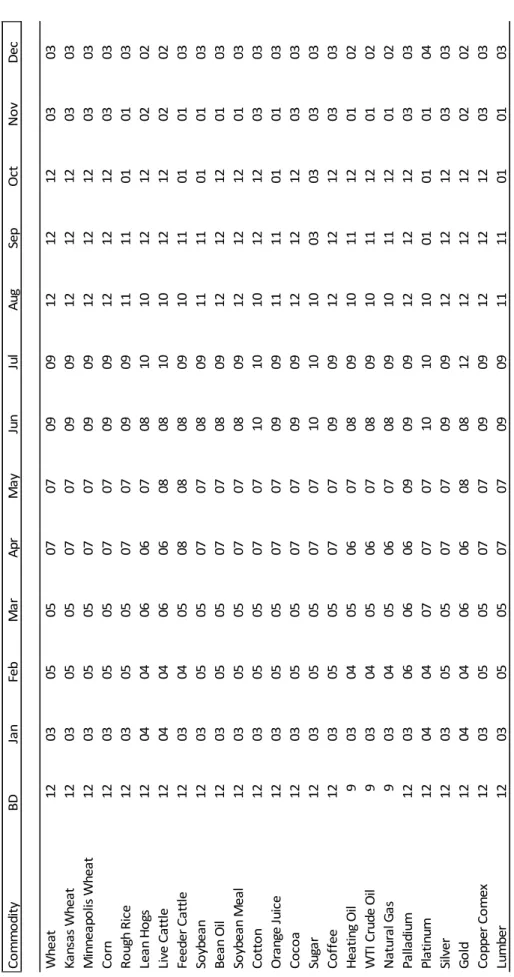
Futures price series are constructed by applying the rollover procedure which is familiar in

the empirical commodity literature. The contracts are rolled into the next available maturity

in the month where the shortest contract expires; a fixed business day is selected for the

rollover. The roll schedule applied to each commodity is displayed in Table APP1 in the Ap‐

pendix. Using Wheat as an example, the contract is rolled on the 12th business day of Febru‐

ary, where the expiration month switches from March to May. On the 12th business day of

April, the expiration month switches from May to July. This expiration applies until the 12th

business day in June, where the expiration month switches to September, and so on.

All prices are denoted in U.S. dollars and were downloaded from Thomson Reuters

Datastream. In order to match returns with the weekly position data available from the CFTC

commitment of traders (COT) reports used for our speculation proxies, we compute weekly

Tuesday‐to‐Tuesday log returns.

Granger causality (GC) tests

We apply standard Granger causality tests to weekly return and position data, and respec‐

tively, weekly return variances and position data. Returns are measured as log changes of

Tuesday closing prices, and weekly variances are proxied by quadratic log returns.14

The timing of the variables needs some explanation; it is surprising that this crucial topic is

mostly not addressed in empirical studies.15 The weekly published COT‐ (and SCOT‐) reports

contain the position data on Tuesday, but they are not released until Friday. Depending on

how well and quick information is processed in commodity markets, the release may have an

impact on prices. If there is an information (aggregation) effect, the Tuesday‐positions in t

14_This_is_justified_if_the_measurement_interval_is_„small“_and_the_expected_return_is_close_to_zero._Since_in_gen_‐

eral the variability of commodity returns seems to dominate expectations (risk premiums), this procedure

seems adequate to us even if a week is not strictly a “small” time interval.

15_A_notable_exception_is_Sanders,_Boris,_and_Manfredo_(2004);_the_study_reveals_that_the_timing_of_the_COT_data

(8)

(released a few days later) would have predictive power for the weekly futures return from t

to t+1, but this effect is unrelated to the economic causation of speculative positions on sub‐

sequent returns and volatility. In this case, in order to stay conservative towards finding

causal effects running from positions to returns and volatilities, it would be preferable to

consider the positions in t (released a few days later) and the subsequent returns from t+1 to

t+2 as “contemporaneous”. However, if markets are efficient and information is processed in

the market without publication lag, this procedure would wash out a possible causal effect.

In this case, we should consider the positions in t and the returns from t to t+1 as contempo‐

raneous. Since there is no direct evidence about a publication effect in the literature, we

chose the second “efficient market” view.16

The optimal lag lengths from the VAR used in the GC tests are determined from the Schwarz

criterions (SC).

The VAR estimation results are used to perform a variance decomposition for those cases

where the null of no‐causality from speculation to returns or volatilities can be rejected. A

Cholesky decomposition is applied to the error matrix. With respect to the ordering of varia‐

bles, the speculation proxy is selected as the first variable, the returns as second. In our Ta‐

bles, we only display the maximum variance share in the returns explained by the specula‐

tion proxy across the periods.

3. Descriptive Statistics

Table 1 (Panels A to C) provides descriptive statistics of the three speculation proxies. We

skip the statistics of the futures returns because they are widely documented in the empiri‐

cal literature, and they are not substantially different for our sample.

The autocorrelation coefficients are reported in the past three columns; they are significant‐

ly different from zero (indicated by bold figures) across all proxies and commodities. Most of

the AC(1) coefficients are close to one and decrease slowly, which indicates a degree of per‐

sistence in most series. Since the application of standard Granger causality tests requires

stationary data, we have to test for a unit root. Of course, one could argue that the three

measures represent relative shares of speculation and exhibit upper and lower bounds by

definition, and thus the series are stationary by construction. However, in finite samples, the

series can well fluctuate in a range of values such that tests are unable to reject the null of a

unit root.

The results of ADF unit root tests for non‐stationarity are displayed in Table 2. They confirm

that non‐stationarity cannot be rejected in about one third of the cases (on a 99% confi‐

16

Of course, this problem prevails whenever a stock variable (positions) must be matched with flow variables

(returns or volatilities) – even without publication lags. Taking first differences of the position data over the

weekly return measurement interval does not solve the problem, since our hypotheses to be tested are explic‐

(9)

dence level, using the Schwarz criterion), i.e. they behave as if they are non‐stationary. The

detailed results for the three proxies are displayed in separate panels of the Table: Panel A

(Working index WT), Panel B (speculative open interest SOI), and Panel C (speculation pres‐

sure SP), each subdivided for COT‐ and SCOT‐based measures (A1, A2, B1 etc.). On a 99% (in

parentheses: 90%) significance level, the null of a unit root cannot be rejected in 10 (4), 7 (3)

and 11 (4) of the 28 COT series, and in 7 (3), 5 (1) and 4 (0) of the 16 SCOT series. Thus, there

is evidence for non‐stationarity, but in most cases only on relatively low significance level.

Since the construction of the speculation proxies is fairly different, it is not surprising that

the time series characteristics are different across proxies and commodities. Only KC and CL

are non‐stationary across all three proxies.

In the cases where we are unable to reject a unit root with 99% confidence, an augmented

test of GC must be applied as suggested by Toda and Yamamoto (1995), which takes into

account the maximum order of integration of the non‐stationary variable (which is 1 in

our case), which must be added to the optimal lag length of the original VAR model. Howev‐

er, the GC null hypothesis is tested on only the original number of lags. Our empirical results

rely on the T‐Y test where it is appropriate.

4. Empirical findings

4.1 Speculative effects on returns

How does speculation affect realized returns (log price change) in subsequent periods? The

results for the three speculation proxies are displayed in Table 3, Panels A to C, each subdi‐

vided for the COT‐ and SCOT‐based measures (A1, A2, B1 etc.). The general observation is

that the number of significant effects running from speculation to returns is small. Where

such an effect is found (on the 10% significance level), two summary statistics are reported

in the last column of each Panel, headed by “VAR / variance decomposition”: first, a coeffi‐

cient which indicates the sign of the relationship (sum of VAR parameter), and a coefficient

which shows the percentage return variance explained by speculation.

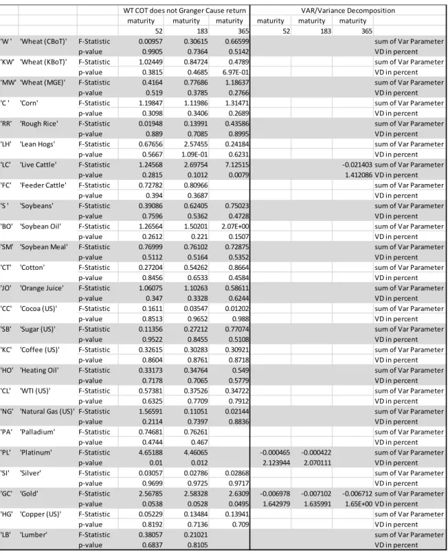
 If speculation is measured by the Working WT index, 3 (2) commodities and 6 (2) ma‐

turities exhibit a significant relationship, which is negative in all cases. Thus, more

unnecessary speculation Granger causes lower returns, i.e. futures price to decrease.

The explained variance is below 2.2%. There is an overlap of significant effects for the

COT and SCOT speculation proxies for a single commodity only: live cattle (for the

longest maturity).

 In the case of speculative open interest (SOI) as speculation measure, 6 (6) commodi‐

ties and 14 (12) maturities exhibit a significant relationship, which is negative without

exception. That is, more speculation is associated with lower returns. However, the

(10)

using the SCOT series where explanatory power is in the range of 6% to 6.5%. There

is an overlap of significant effects for the COT and SCOT speculation proxies for 2

commodities: live cattle (for the longest maturity) and cotton (for all 3 maturities).

Overall, the SOI proxy seems to have the most pronounced effects for agricultural fu‐

tures (cotton, wheat, corn, rice) among all the measures.

 If speculative pressure (SP) is used as speculation measure, i.e. if the sign of net

speculation is taken into account, 4 (4) commodities and 8 (8) maturities exhibit a

significant relationship, which is positive except in a single case. That is, positive

speculation pressure (an overhang of long positions) is associated with higher returns

(futures prices increase), negative pressure is associated with lower returns (futures

price decrease). The maximum explained variance is 2.8%. There is an overlap of sig‐

nificant effects for the COT and SCOT speculation proxies for 2 commodities: live cat‐

tle (for the longest maturity) and coffee (for the second and third maturity).

Overall, the results can be interpreted as follows: Positive Granger causality effects of specu‐

lation on subsequent returns (i.e. positive price effects) can only be found for the specula‐

tion pressure (SP) measure. Thus, it appears that the sign of net speculation seems to have

some explanatory power for this sign of subsequent returns. For the SCOT‐based proxies,

with a stronger bias towards speculation, the effect can be observed across all three maturi‐

ties for BO (soybean oil) and KC (coffee), and for a single maturity for LC (live cattle) and LH

(lean hogs). The effect for and KC and LC can also be observed for the more conservative

COT‐based proxy. However, the explained variance is not more than 2.8%.

In all the other tests, more speculation leads to lower subsequent returns. This is particularly

true for SOI as a proxy variable, so that the general claim that “more speculation” leads to

higher prices does not seem to be justified. However, the proxy is only of limited economic

relevance. But the Working index does not reveal positive effects either: Significant negative

effects are just observed in the SCOT data for a single maturity in two commodities (LH and

LC, again), and all the other significant effects are observed in the COT data in precious met‐

als, with the exception of a single maturity for LC (again). The explained variance of WT for

LH and LC is again some 1.5%.

It does not appear that the SCOT‐based speculation measures, which are more biased to‐

wards speculation, exhibit stronger effects, quite the contrary is true. This means that OTC

index investing – measured indirectly through the activity of index swap dealers ‐ does not

seem to have an impact on our findings. It is interesting to observe that several significant

effects are observed – across all three measures, although for all maturities – for live cattle

and lean hogs (for 13 maturities out of 36); there is no other study which reports this finding.

Although significant Granger causality effects are found, the explained return variance is

small, with a typical value between 1% and 2%. Thus, speculation does not seem to be a ma‐

jor individual driver of commodity futures returns. The “public” perception, that more specu‐

(11)

a single proxy (net speculation pressure), but the other two proxies lead to opposite conclu‐

sions.

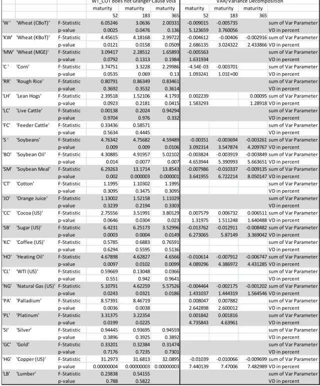
4.2 Speculative effects on variance

How does speculation affect the variance of realized returns in subsequent periods? Here,

the mere inspection of the results displayed in Table 4 (Panels A to C, which have the same

structure as in the previous Table) reveals that the number of statistically significant effects

is much larger than in the results for returns reported before. We find statistically significant

effects for 40% (34%) of the analyzed contract maturities if COT (SCOT) data is used.17 Also,

the results are more mixed across the individual commodities. The findings can be summa‐

rized as follows:

 If speculation is measured by the Working WT index, 15 (7) commodities and 38 (18)

maturities exhibit a significant relationship, which is negative for 11 (5) and positive

for 4 (2) commodities out of 25 (12).18 Thus, for the majority of commodities, more

unnecessary speculation Granger causes lower a lower volatility in the subsequent

weeks. The explained variance does not exceed 8%. There is an overlap of significant

effects for the COT and SCOT speculation proxies for 7 commodities: lean hogs and

cocoa (positive), and Chicago and Kansas wheat, soybean oil and meal, and sugar

(negative).

 For speculative open interest (SOI) as speculation measure, 12 (6) commodities and

28 (11) maturities exhibit a significant relationship, which is negative for 9 (2) and

positive for 3 (4) commodities. Thus, the use of SCOT‐based measures leads to a larg‐

er number of volatility‐increasing effects. The explained variance does not exceed

6%. There is an overlap of significant negative effects for the COT and SCOT specula‐

tion proxies for 2 commodities: Kansas wheat and soybean oil (for all maturities).

 If speculative pressure (SP) is used as proxy, i.e. the sign of net speculation is consid‐

ered to be relevant, 11 (5) commodities and 24 (8) maturities exhibit a significant re‐

lationship, which is negative in 5 (3) and positive in 5 (1) cases.19 Of course, it is a pri‐

ori not clear whether an overhang of long20 or short positions should be associated

with a higher volatility – it could well be that a large overhang with either sign could

be associated with a large volatility; such an effect would imply a non‐linear relation‐

ship and requires a different test procedure. The mixed results (signs) which are in

apparent contrast to those for the other two proxies could be a possible conse‐

quence of such an effect. There is an overlap of significant effects for the COT and

17

Again, a significance level of 90% is selected.

18

The sign of the relationship is the same across all maturities for essentially all commodities, except for LC if

the SP is used as speculation proxy.

19

As stated before, one commodity (LC, life cattle) is indeterminate across maturities.

20

Net long (short) speculation increases (decreases) volatility for e.g. soybean oil and meal, rice, sugar, and

occasionally wheat, while it decreases (increases) volatility for e.g. cocoa, lean hogs, feeder cattle, WTI oil,

(12)

SCOT speculation proxies for 2 commodities, feeder cattle and cocoa (both negative),

however, for a single maturity only.

Overall, the results can be summarized as follows: If speculative open interest is regarded as

valid proxy and SCOT data are analyzed, one would be tempted to conclude more specula‐

tion leads to higher futures price volatility. However, the picture changes completely if the

speculation is related to commercial positions: the WT index indicates a negative volatility

effect for most commodities, except for lean hogs and cocoa. Overall, the results are ex‐

tremely robust across the maturities of the contracts (for positive and negative effects) and

the COT and SCOT data. The only heterogeneous results are reported for the speculation

pressure proxy, which would not be surprising if a non‐linear relationship between SP and

volatility should exist.

In general, the explanatory power of the speculative proxies is considerably higher for the

volatilities than for the returns. However, the fraction of variance explained is in a typical

range of 2‐6% and does not exceed 8%, which indicates a rather limited role of speculative

effects in explaining futures volatility.

4.3 Special results for index commodities?

Are the empirical results stronger for commodities which are included in popular commodity

indices? If index investing has special pricing effects on commodity futures, then the number

of significant effects or the explained variance should be larger for those commodities where

SCOT‐data are available. Moreover, the SCOT‐based speculation proxies should also provide

more precise estimates of speculation. Recall that SCOT statistics were introduced for those

commodities which are subject to significant index trading.

The number of significant results is measured by the total number of contracts (a total of 75

maturities for the 25 COT commodities, and 36 maturities for the 12 SCOT commodities) for

which statistically significant Granger causality is observed on the 10% significance level.

For the return analysis (Table 3), indeed, the number of significant results is larger for the

SCOT data than for the COT data (20% vs. 12%).21 However, this is only true if SP and SOI are

used as speculation proxies, not for the WT index. Therefore, speculation proxies unrelated

to commercial positions might indeed indicate more significant return effects in index‐

related commodities.

In case of the volatility analysis (Table 4), the picture is different: the number of significant

results is smaller for the SCOT data across all three speculation proxies (34% vs. 40%).

21_The_percentages_are_computed_as_simple_averages_across_commodities_and_contracts_(for_each_proxy),_and

(13)

With respect to the explained variance, we observe the following differences between the

COT‐ and SCOT‐results: the mean (and median) explained variance of returns is 2% for the

SCOT data (1.7%) and is slightly larger than for the COT data with 1.6% (1.5%). But apparent‐

ly, the overall figure is small for both datasets. The mean explained variance of volatilities is

virtually identical for the SCOT and COT data, namely 3.1%, and the median is slightly larger

for the SCOT data (3.4% vs. 3.2%).22 Thus, in terms of the explained variance, the SCOT da‐

taset reveals slightly more explanatory power for the speculation proxies, but in absolute

size of the figures does not indicate substantial differences.

We therefore conclude that our empirical findings – in terms of the strength of the observed

causal effects ‐ do not differ substantially between the COT or SCOT datasets. Thus, we do

not find stronger effects for index‐related commodities in our results.

22

A breakdown of the results for the individual speculation proxies, however, reveals that the explanatory

power of the WT index (which we regard as the economically superior proxy) is consistently smaller for the

(14)

5. Summary and conclusions

Granger causality tests are very popular in the current discussion about the role of financial

speculation in commodity futures markets. Unfortunately, the heterogeneity of tests in

terms of speculation proxies, price variables, futures contracts, or analyzed time period

makes it extremely hard to draw meaningful conclusions from the published results. Also,

the focus of many papers is not on individual commodities. The main contribution of our

paper is therefore to apply T‐Y augmented Granger causality tests to a consistent set of fu‐

tures returns and volatilities, for three maturities, using three speculation proxies applied to

two data sources of position data.

Our findings can be summarized as follows: There is a substantial higher degree of spillover

effects from speculation to volatilities than from speculation to returns on futures markets.

In the case of volatilities, we found statistically significant effects in some 40% of the con‐

tracts (COT data), compared to 20% for returns (SCOT data). There is essentially no return

effect if the WT measure is used, some positive effects for the SP measure, and negative for

the SOI measure. The volatility effects are mostly negative, i.e. more speculation is followed

by lower return volatility. This is particularly true if the Working index is used as speculation

proxy which is widely regarded as the most meaningful measure.

Even where statistically significant effects are found, the explained variance is economically

small or at best moderate: the typical values are in the range of 1‐2% (for returns) and 2‐6%

(for volatilities).

With respect to the individual commodities, two observations are striking: First, there are

essentially no destabilizing effects of speculation with respect to agricultural commodity

futures prices. Where significant effects are reported, they rather point to the opposite di‐

rection: more speculation is followed by lower returns (SOI measure) and lower volatilities –

with very few exceptions. Second, destabilizing effects, if any, are more frequently observed

in livestock, in particular live cattle and lean hogs: the signs in the return effects are however

mixed, but for several volatility effects are positive (for the WT and OI proxies, in the COT

and SCOT data). This might be the first study to find effects in this commodity group with

some persistence.

There is some – but less conclusive – evidence for some destabilizing effects for the soft

commodities: coffee futures returns react positively to SP, but no volatility effects are ob‐

served. For sugar, negative and positive volatility effects are observed (negative for WT, pos‐

itive for SOI). Cocoa volatility reacts positively to speculation measured by WT, but not to the

other two proxies. Thus, the overall picture is mixed here.

(15)

References

Cootner, Paul H. (1960): Returns to speculators: Telser versus Keynes, Journal of Political

Economy 68, pp. 396‐404.

Gilbert, Christopher L., and Simone Pfuderer (2014): The financialization of food commodity

markets. Handbook on Food: Demand, Supply, Sustainability and Security (edited by

Raghbendra Jha, Raghav Gaiha and Anil B. Deolalikar), Elgar, pp. 122‐48.

Haase, Marco, Yvonne Seiler, and Heinz Zimmermann (2015): Permanent and transitory

price shocks in commodity futures markets and their relation to storage and speculation,

ssrn‐Working Paper, WWZ Uni Basel, January

Lehecka, Georg V. (2015): Do hedging and speculative pressures drive commodity prices, or

the other way round? Empirical Economics 49, pp. 575‐603

Sanders, Dwight R., Scott H. Irwin, and Robert P. Merrin (2010): The adequacy of speculation

in agricultural futures markets: Too much of a good thing? Applied Economic Perspectives

and Policy 32, pp. 77‐94

Sanders, Dwight R., Keith Boris, and Mark Manfredo (2004): Hedgers, funds, and small

speculators in the energy futures markets: an analysis of the CFTC's Commitments of Traders

reports, Energy Economics 26, pp. 425‐445.

Stoll, Hans and Robert Whaley (2011): Commodity index investing: Speculation or diversifica‐

tion?, Journal of Alternative Investments 14 (Summer), pp. 50‐60.

Toda, Hiro Y., and Taku Yamamoto (1995): Statistical inference in vector autoregressions

with possibly integrated processes, Journal of Econometrics 66, pp. 225‐250.

Working, Holbrook (1960): Speculation on hedging markets, Food Research Institute Studies

2, pp. 185‐220.

(16)

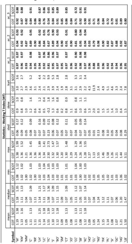
Table 1: Descriptive Statistics

The table displays descriptive statistics of the levels of the three speculation proxies used in this paper: Working T‐

index WT, relative speculative open interest SOI, and speculation pressure SP. The construction of the measures is

described in Section 2 in the text. The abbreviations of commodities are clarified in Table 2. The statistical measures

(mean, median, etc.) are standard. The extensions “cot” and “scot” of the speculation proxies refer to the CFTC posi‐

tion data releases (cot: Commitments of Traders Report, and “scot”: Supplemental Commitments of Traders Report

which contains a reclassification of “index traders”). A confidence level of 90% is applied to autocorrelation coeffi‐

cient, and significant values are displayed in bold. Weekly data are used which cover the period from January 2006 to

March 2015.

Panel A: Working T‐Index, WT

Sy m b o l CO T SCO T C O T SC O T CO T SCO T C O T SC O T CO T SCO T C O T SC O T CO T SCO T C O T SC O T CO T SCO T C O T SC O T 'W ' 1.1 9 1.3 8 1. 18 1 .3 5 1.0 8 1.1 2 1. 38 1 .9 9 0.0 6 0.1 7 0. 9 1 .0 3.0 3. 6 0. 97 0 .97 0. 94 0. 9 3 0. 92 0 .88 'K W ' 1. 13 1. 1 6 1. 11 1 .13 1. 02 1. 0 2 1. 36 1 .52 0. 09 0. 1 2 0. 8 0 .8 2. 7 2. 7 0. 96 0 .97 0. 92 0. 9 2 0. 87 0 .88 'M W ' 1. 05 Na N 1. 04 Na N 1. 00 Na N 1. 21 Na N 0. 05 Na N 1. 0 Na N 2. 9 Na N 0. 93 0. 00 0. 87 0. 0 0 0. 82 0. 00 'C ' 1.1 1 1.1 3 1. 07 1 .0 9 1.0 2 1.0 3 1. 36 1 .4 5 0.0 8 0.0 9 1. 2 1 .6 3.6 5. 2 0. 94 0 .98 0. 89 0. 9 5 0. 84 0 .91 'R R ' 1. 11 Na N 1. 11 Na N 1. 00 Na N 1. 36 Na N 0. 07 Na N 0. 6 Na N 3. 1 Na N 0. 95 0. 00 0. 90 0. 0 0 0. 86 0. 00 'L H ' 1. 15 1. 2 5 1. 14 1 .21 1. 02 1. 0 3 1. 36 1 .89 0. 07 0. 1 6 0. 4 1 .2 2. 4 4. 4 0. 94 0 .97 0. 86 0. 9 2 0. 80 0 .87 'L C ' 1. 14 1. 1 8 1. 11 1 .17 1. 03 1. 0 4 1. 34 1 .41 0. 07 0. 0 9 0. 5 0 .4 2. 1 2. 2 0. 92 0 .96 0. 84 0. 9 1 0. 76 0 .86 'F C ' 1. 55 1. 3 9 1. 58 1 .36 1. 04 1. 0 5 2. 30 2 .73 0. 23 0. 2 1 ‐ 0. 2 1 .8 2. 9 9. 9 0. 81 0 .86 0. 67 0. 7 6 0. 54 0 .65 'S ' 1.1 0 1.1 2 1. 07 1 .0 9 1.0 3 1.0 3 1. 32 1 .4 7 0.0 6 0.0 8 1. 3 1 .6 3.9 5. 3 0. 95 0 .96 0. 89 0. 9 0 0. 84 0 .85 'B O' 1. 12 1. 1 8 1. 11 1 .15 1. 02 1. 0 3 1. 30 1 .57 0. 07 0. 1 2 0. 6 0 .8 2. 4 2. 8 0. 97 0 .97 0. 94 0. 9 3 0. 91 0 .89 'S M ' 1. 09 Na N 1. 09 Na N 1. 01 Na N 1. 20 Na N 0. 05 Na N 0. 2 Na N 1. 9 Na N 0. 95 0. 00 0. 90 0. 0 0 0. 85 0. 00 'C T' 1. 09 1. 1 3 1. 07 1 .09 1. 01 1. 0 1 1. 30 1 .48 0. 07 0. 1 1 0. 8 0 .9 2. 8 2. 8 0. 97 0 .97 0. 91 0. 9 1 0. 86 0 .85 'J O' 1. 08 Na N 1. 05 Na N 1. 01 Na N 1. 29 Na N 0. 07 Na N 1. 1 Na N 3. 1 Na N 0. 96 0. 00 0. 90 0. 0 0 0. 84 0. 00 'C C ' 1. 11 1. 1 3 1. 11 1 .12 1. 03 1. 0 4 1. 24 1 .29 0. 04 0. 0 5 0. 6 0 .8 3. 1 3. 3 0. 92 0 .90 0. 81 0. 8 0 0. 71 0 .72 'S B ' 1. 08 1. 1 1 1. 05 1 .07 1. 00 1. 0 0 1. 26 1 .36 0. 07 0. 0 9 1. 0 1 .1 2. 9 3. 1 0. 98 0 .98 0. 95 0. 9 4 0. 92 0 .91 'K C ' 1. 12 1. 1 8 1. 10 1 .14 1. 02 1. 0 3 1. 28 1 .55 0. 07 0. 1 4 0. 6 1 .1 2. 2 3. 4 0. 97 0 .98 0. 94 0. 9 4 0. 90 0 .91 'H O' 1. 09 Na N 1. 07 Na N 1. 02 Na N 1. 27 Na N 0. 05 Na N 1. 3 Na N 4. 3 Na N 0. 96 0. 00 0. 93 0. 0 0 0. 91 0. 00 'C L' 1. 05 Na N 1. 04 Na N 1. 03 Na N 1. 13 Na N 0. 01 Na N 2. 0 Na N 11. 9 Na N 0. 88 0. 00 0. 79 0. 0 0 0. 71 0. 00 'N G ' 1. 24 Na N 1. 24 Na N 1. 05 Na N 1. 55 Na N 0. 13 Na N 0. 3 Na N 2. 4 Na N 0. 99 0. 00 0. 98 0. 0 0 0. 96 0. 00 'P A ' 1. 15 Na N 1. 12 Na N 1. 05 Na N 1. 46 Na N 0. 08 Na N 1. 5 Na N 4. 9 Na N 0. 96 0. 00 0. 90 0. 0 0 0. 84 0. 00 'P L' 1. 14 Na N 1. 11 Na N 1. 02 Na N 1. 58 Na N 0. 10 Na N 1. 5 Na N 5. 1 Na N 0. 92 0. 00 0. 82 0. 0 0 0. 72 0. 00 'S I' 1. 08 Na N 1. 07 Na N 1. 01 Na N 1. 26 Na N 0. 05 Na N 1. 4 Na N 4. 6 Na N 0. 94 0. 00 0. 87 0. 0 0 0. 79 0. 00 'G C ' 1. 07 Na N 1. 06 Na N 1. 03 Na N 1. 21 Na N 0. 04 Na N 1. 0 Na N 3. 3 Na N 0. 94 0. 00 0. 88 0. 0 0 0. 81 0. 00 'H G ' 1. 21 Na N 1. 20 Na N 1. 06 Na N 1. 44 Na N 0. 08 Na N 0. 4 Na N 2. 4 Na N 0. 96 0. 00 0. 92 0. 0 0 0. 89 0. 00 'L B ' 1. 50 Na N 1. 47 Na N 1. 02 Na N 3. 11 Na N 0. 29 Na N 1. 5 Na N 7. 8 Na N 0. 95 0. 00 0. 87 0. 0 0 0. 80 0. 00 ac _ 3 St a ti st ic s ‐ Wo rk in g T In d ex (W T) sk ew ku rt a c_1 ac _2 m ean m e di an m in m a x st ed

(17)

Panel B: Speculative Open Interest, SOI

(18)

Panel C: Speculative Pressure, SP

(19)

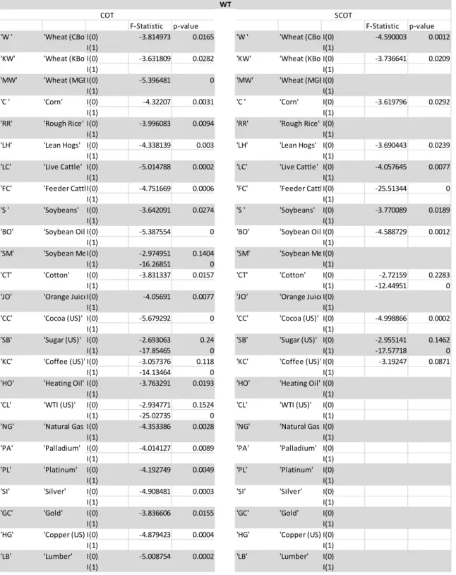
Table 2: Unit root tests for speculation proxies

The table contains ADF (augmented Dickey Fuller) test statistics of unit root tests for the three speculation proxies

used in this paper: The F‐statistic and its p‐value test the null hypothesis of no‐stationarity. If the null of non‐

stationarity for the levels cannot be rejected with 90% confidence (as displayed on the respective first row, I(0) ),

then the test is also applied to first differences and the results are displayed in the second row labelled as I(1). The

results are displayed in separate Panels for three speculation proxies: Working T‐index WT (Panel A), relative specula‐

tive open interest SOI (Panel B), and speculation pressure SP (Panel C). The construction of the measures is described

in Section 2 in the text. Each speculation proxy is calculated with CFTC position data from two data sources: the COT

Commitments of Traders Reports, and SCOT Supplemental Commitments of Traders Reports which contains a reclas‐

sification of “index traders”. Weekly data are used which cover the period from January 2006 to March 2015.

Panel A: Working T‐Index, WT

F‐Statistic p‐value F‐Statistic p‐value 'W ' 'Wheat (CBoTI(0) ‐3.814973 0.0165 'W ' 'Wheat (CBoTI(0) ‐4.590003 0.0012 I(1) I(1) 'KW' 'Wheat (KBoTI(0) ‐3.631809 0.0282 'KW' 'Wheat (KBoTI(0) ‐3.736641 0.0209 I(1) I(1) 'MW' 'Wheat (MGEI(0) ‐5.396481 0 'MW' 'Wheat (MGEI(0) I(1) I(1)

'C ' 'Corn' I(0) ‐4.32207 0.0031 'C ' 'Corn' I(0) ‐3.619796 0.0292

I(1) I(1)

'RR' 'Rough Rice' I(0) ‐3.996083 0.0094 'RR' 'Rough Rice' I(0)

I(1) I(1)

'LH' 'Lean Hogs' I(0) ‐4.338139 0.003 'LH' 'Lean Hogs' I(0) ‐3.690443 0.0239

I(1) I(1)

'LC' 'Live Cattle' I(0) ‐5.014788 0.0002 'LC' 'Live Cattle' I(0) ‐4.057645 0.0077

I(1) I(1)

'FC' 'Feeder CattlI(0) ‐4.751669 0.0006 'FC' 'Feeder Cattl I(0) ‐25.51344 0

I(1) I(1)

'S ' 'Soybeans' I(0) ‐3.642091 0.0274 'S ' 'Soybeans' I(0) ‐3.770089 0.0189

I(1) I(1)

'BO' 'Soybean Oil I(0) ‐5.387554 0 'BO' 'Soybean Oil I(0) ‐4.588729 0.0012

I(1) I(1)

'SM' 'Soybean MeI(0) ‐2.974951 0.1404 'SM' 'Soybean Me I(0)

I(1) ‐16.26851 0 I(1)

'CT' 'Cotton' I(0) ‐3.831337 0.0157 'CT' 'Cotton' I(0) ‐2.72159 0.2283

I(1) I(1) ‐12.44951 0

'JO' 'Orange JuiceI(0) ‐4.05691 0.0077 'JO' 'Orange JuiceI(0)

I(1) I(1)

'CC' 'Cocoa (US)' I(0) ‐5.679292 0 'CC' 'Cocoa (US)' I(0) ‐4.998866 0.0002

I(1) I(1)

'SB' 'Sugar (US)' I(0) ‐2.693063 0.24 'SB' 'Sugar (US)' I(0) ‐2.955141 0.1462

I(1) ‐17.85465 0 I(1) ‐17.57718 0

'KC' 'Coffee (US)' I(0) ‐3.057376 0.118 'KC' 'Coffee (US)' I(0) ‐3.19247 0.0871

I(1) ‐14.13464 0 I(1)

'HO' 'Heating Oil' I(0) ‐3.763291 0.0193 'HO' 'Heating Oil' I(0)

I(1) I(1)

'CL' 'WTI (US)' I(0) ‐2.934771 0.1524 'CL' 'WTI (US)' I(0)

I(1) ‐25.02735 0 I(1)

'NG' 'Natural Gas I(0) ‐4.353386 0.0028 'NG' 'Natural Gas I(0)

I(1) I(1)

'PA' 'Palladium' I(0) ‐4.014127 0.0089 'PA' 'Palladium' I(0)

I(1) I(1)

'PL' 'Platinum' I(0) ‐4.192749 0.0049 'PL' 'Platinum' I(0)

I(1) I(1)

'SI' 'Silver' I(0) ‐4.908481 0.0003 'SI' 'Silver' I(0)

I(1) I(1)

'GC' 'Gold' I(0) ‐3.836606 0.0155 'GC' 'Gold' I(0)

I(1) I(1)

'HG' 'Copper (US) I(0) ‐4.879423 0.0004 'HG' 'Copper (US) I(0)

I(1) I(1)

'LB' 'Lumber' I(0) ‐5.008754 0.0002 'LB' 'Lumber' I(0)

I(1) I(1)

WT

(20)

Panel B: Speculative Open Interest, SOI

F‐Statistic p‐value F‐Statistic p‐value 'W ' 'Wheat (CBoTI(0) ‐3.71382 0.0223 'W ' 'Wheat (CBoTI(0) ‐3.495004 0.041 I(1) I(1) 'KW' 'Wheat (KBoTI(0) ‐3.96538 0.0104 'KW' 'Wheat (KBoTI(0) ‐3.971232 0.0102 I(1) I(1) 'MW' 'Wheat (MGEI(0) ‐2.626392 0.2687 'MW' 'Wheat (MGEI(0) I(1) ‐22.45215 0 I(1)

'C ' 'Corn' I(0) ‐5.23808 0.0001 'C ' 'Corn' I(0) ‐5.186743 0.0001

I(1) I(1)

'LC' 'Live Cattle' I(0) ‐5.388334 0 'LC' 'Live Cattle' I(0) ‐4.158575 0.0055

I(1) I(1)

'FC' 'Feeder Cattl I(0) ‐4.615782 0.0011 'FC' 'Feeder Cattl I(0) ‐4.062982 0.0076

I(1) I(1)

'S ' 'Soybeans' I(0) ‐6.655633 0 'S ' 'Soybeans' I(0) ‐5.680997 0

I(1) I(1)

'BO' 'Soybean Oil I(0) ‐5.599974 0 'BO' 'Soybean Oil I(0) ‐4.823318 0.0005

I(1) I(1)

'SM' 'Soybean Me I(0) ‐4.916506 0.0003 'SM' 'Soybean Me I(0)

I(1) I(1)

'JO' 'Orange JuiceI(0) ‐6.157663 0 'JO' 'Orange JuiceI(0)

I(1) I(1)

'CC' 'Cocoa (US)' I(0) ‐4.524428 0.0015 'CC' 'Cocoa (US)' I(0) ‐4.192974 0.0049

I(1) I(1)

'SB' 'Sugar (US)' I(0) ‐5.572807 0 'SB' 'Sugar (US)' I(0) ‐4.575224 0.0012

I(1) I(1)

I(1) ‐6.024555 0 I(1) ‐5.779638 0

I(1) I(1)

I(1) ‐15.05055 0 I(1)

I(1) I(1)

'SI' 'Silver' I(0) ‐4.811921 0.0005 'SI' 'Silver' I(0)

I(1) I(1)

'GC' 'Gold' I(0) ‐4.335998 0.003 'GC' 'Gold' I(0)

I(1) I(1)

'HG' 'Copper (US) I(0) ‐5.588393 0 'HG' 'Copper (US) I(0)

I(1) I(1)

SOI

(21)

Panel C: Speculative Pressure, SP

F‐Statistic p‐value F‐Statistic p‐value 'W ' 'Wheat (CBoTI(0) ‐5.223423 0.0001 'W ' 'Wheat (CBoTI(0) ‐5.627741 0 I(1) I(1) 'KW' 'Wheat (KBoTI(0) ‐4.270751 0.0038 'KW' 'Wheat (KBoTI(0) ‐4.721007 0.0007 I(1) I(1) 'MW' 'Wheat (MGEI(0) ‐4.291186 0.0035 'MW' 'Wheat (MGEI(0) I(1) I(1)

'C ' 'Corn' I(0) ‐4.359639 0.0027 'C ' 'Corn' I(0) ‐4.261138 0.0039

I(1) I(1)

'LC' 'Live Cattle' I(0) ‐3.88488 0.0134 'LC' 'Live Cattle' I(0) ‐3.686567 0.0241

I(1) I(1)

'FC' 'Feeder CattlI(0) ‐3.947699 0.011 'FC' 'Feeder Cattl I(0) ‐3.662142 0.0259

I(1) I(1)

'S ' 'Soybeans' I(0) ‐3.740995 0.0206 'S ' 'Soybeans' I(0) ‐4.17631 0.0052

I(1) I(1)

'BO' 'Soybean Oil I(0) ‐4.809005 0.0005 'BO' 'Soybean Oil I(0) ‐4.711666 0.0007

I(1) I(1)

'SM' 'Soybean MeI(0) ‐3.6585 0.0261 'SM' 'Soybean Me I(0)

I(1) I(1)

'JO' 'Orange JuiceI(0) ‐2.731033 0.2245 'JO' 'Orange JuiceI(0)

I(1) ‐17.16197 0 I(1)

'CC' 'Cocoa (US)' I(0) ‐4.071245 0.0074 'CC' 'Cocoa (US)' I(0) ‐4.302088 0.0034

I(1) I(1)

'SB' 'Sugar (US)' I(0) ‐4.206944 0.0047 'SB' 'Sugar (US)' I(0) ‐5.180066 0.0001

I(1) I(1)

I(1) ‐23.78016 0 I(1)

I(1) I(1)

'SI' 'Silver' I(0) ‐5.617024 0 'SI' 'Silver' I(0)

I(1) I(1)

'GC' 'Gold' I(0) ‐4.014484 0.0089 'GC' 'Gold' I(0)

I(1) I(1)

'HG' 'Copper (US) I(0) ‐3.028388 0.1255 'HG' 'Copper (US) I(0)

I(1) ‐17.58599 0 I(1)

I(1) I(1)

SP

(22)

Table 3: Speculative effects on returns

The table contains the results of Granger causality tests (respectively, Y‐T augmented Granger causality tests where

the speculation proxy is non‐stationary) that speculative positions do not “cause” subsequent futures returns. The F‐

statistic and p‐value of the test are displayed in the third 4th to 6th columns. For those cases where a significant

effect is found with 90% confidence, the results of a variance decomposition is displayed in the 7th to 9th columns,

which show the impact (sum of the VAR parameters) and explained variance (in percentages). The results are dis‐

played in separate Panels for three speculation proxies: Working T‐index WT (Panel A), relative speculative open

interest SOI (Panel B), and speculation pressure SP (Panel C). The construction of the measures is described in Section

2 in the text. Each speculation proxy is calculated with CFTC position data from two data sources: the COT Commit‐

ments of Traders Reports, and SCOT Supplemental Commitments of Traders Reports which contains a reclassification

of “index traders” (Subpanels A1, A2, etc.). The abbreviations of commodities are clarified in Table 2. Weekly data are

used which cover the period from January 2006 to March 2015.

Panel A1: Working T‐Index, WT COT

maturity maturity maturity maturity maturity maturity

52 183 365 52 183 365

'W ' 'Wheat (CBoT)' F‐Statistic 0.00957 0.30615 0.66599 sum of Var Parameter p‐value 0.9905 0.7364 0.5142 VD in percent 'KW' 'Wheat (KBoT)' F‐Statistic 1.02449 0.84724 0.4789 sum of Var Parameter

p‐value 0.3815 0.4685 6.97E‐01 VD in percent 'MW' 'Wheat (MGE)' F‐Statistic 0.4164 0.77686 1.18637 sum of Var Parameter

p‐value 0.519 0.3785 0.2766 VD in percent 'C ' 'Corn' F‐Statistic 1.19847 1.11986 1.31471 sum of Var Parameter

p‐value 0.3098 0.3406 0.2689 VD in percent 'RR' 'Rough Rice' F‐Statistic 0.01948 0.13991 0.43586 sum of Var Parameter

p‐value 0.889 0.7085 0.8995 VD in percent 'LH' 'Lean Hogs' F‐Statistic 0.67656 2.57455 0.24184 sum of Var Parameter

p‐value 0.5667 1.09E‐01 0.6231 VD in percent 'LC' 'Live Cattle' F‐Statistic 1.24568 2.69754 7.12515 ‐0.021403 sum of Var Parameter

p‐value 0.2815 0.1012 0.0079 1.412086 VD in percent 'FC' 'Feeder Cattle' F‐Statistic 0.72782 0.80966 sum of Var Parameter

p‐value 0.394 0.3687 VD in percent

'S ' 'Soybeans' F‐Statistic 0.39086 0.62405 0.75023 sum of Var Parameter p‐value 0.7596 0.5362 0.4728 VD in percent 'BO' 'Soybean Oil' F‐Statistic 1.26564 1.50201 2.07E+00 sum of Var Parameter

p‐value 0.2612 0.221 0.1507 VD in percent 'SM' 'Soybean Meal' F‐Statistic 0.76999 0.76102 0.72875 sum of Var Parameter

p‐value 0.5112 0.5164 0.5352 VD in percent 'CT' 'Cotton' F‐Statistic 0.27204 0.54262 0.8664 sum of Var Parameter

p‐value 0.8456 0.6533 0.4584 VD in percent 'JO' 'Orange Juice' F‐Statistic 1.06075 1.10263 0.58611 sum of Var Parameter

p‐value 0.347 0.3328 0.6244 VD in percent 'CC' 'Cocoa (US)' F‐Statistic 0.1611 0.03547 0.01202 sum of Var Parameter

p‐value 0.8513 0.9652 0.988 VD in percent 'SB' 'Sugar (US)' F‐Statistic 0.11356 0.27212 0.77074 sum of Var Parameter

p‐value 0.9522 0.8455 0.5108 VD in percent 'KC' 'Coffee (US)' F‐Statistic 0.32615 0.30283 0.30921 sum of Var Parameter

p‐value 0.8604 0.8761 0.8718 VD in percent 'HO' 'Heating Oil' F‐Statistic 0.33173 0.34764 0.549 sum of Var Parameter

p‐value 0.7178 0.7065 0.5779 VD in percent 'CL' 'WTI (US)' F‐Statistic 0.57381 0.37526 0.34722 sum of Var Parameter

p‐value 0.6325 0.7709 0.7912 VD in percent 'NG' 'Natural Gas (US)' F‐Statistic 1.56591 0.11051 0.02144 sum of Var Parameter

p‐value 0.2114 0.7397 0.8836 VD in percent 'PA' 'Palladium' F‐Statistic 0.74681 0.76261 sum of Var Parameter

'PL' 'Platinum' F‐Statistic 4.65188 4.46065 ‐0.000465 ‐0.000422 sum of Var Parameter p‐value 0.01 0.012 2.123944 2.070111 VD in percent 'SI' 'Silver' F‐Statistic 0.03057 0.02786 0.02868 sum of Var Parameter

p‐value 0.9699 0.9725 0.9717 VD in percent 'GC' 'Gold' F‐Statistic 2.56785 2.58328 2.6309 ‐0.006978 ‐0.007102 ‐0.006712 sum of Var Parameter

p‐value 0.0538 0.0528 0.0495 1.642979 1.635991 1.65E+00 VD in percent 'HG' 'Copper (US)' F‐Statistic 0.05229 0.13484 0.13941 sum of Var Parameter

p‐value 0.8192 0.7136 0.709 VD in percent 'LB' 'Lumber' F‐Statistic 0.38057 0.21021 sum of Var Parameter

VAR/Variance Decomposition WT COT does not Granger Cause return