Effect of Strip-Cast Micro-Segregation on Phase
Transformations in Medium to High-Carbon Steels
by
Jerome Cornu
Submitted in fulfilment of the requirements for the degree of Doctor of Philosophy
Deakin University April, 2018
Acknowledgements
Upon completing this work, many people should be personally acknowledged. First and foremost, I would like to thank my supervisors A.Prof. Nicole Stanford, Dr. Thomas Dorin and Prof. Peter Hodgson for giving me the opportunity to take part in the PhD journey, as well as in the most valuable local and international experiences: experiments, conferences and workshops made this time all the more exciting and rewarding on both personal and professional levels. Thanks for your guidance and support during the course of this work.
Many thanks go to the post‐doctoral and technical staff at the IFM for their constant help and support: Dr. Andrew Sullivan, Dr. Mark Nave, Dr. Adam Taylor and Rosey Squire for sharing their skills on characterisation techniques, Rob Pow, Huaying (Maggie) Yin, John Vella, Lynton Leigh, Steve Mills and Mohan Setty for their regular help in the lab, Dr. Ross Marceau and Dr. Hossein Beladi for helping out on the project on many occasions. Special thanks to David Gray who made alloy casting the most entertaining experiments I have ever assisted: thanks for sharing your great playlists and surfing tips.
I owe my gratitude to many people outside of the IFM as well: Prof. Christopher Hutchinson and Yuxiang Wu at Monash University for kindly sharing their experience with Thermocalc, Dr. Paul Guagliardo for the helpful collaborative work at UWA and Prof. Bevis Hutchinson for his much appreciated insight on various aspects of the project.
Many fellow PhD students should be thanked for helping out on many levels. Sharing personal experiences and tips was the best support and made the times of doubt all the more bearable. In this regard and to only name a few, my appreciation goes to Lu Jiang, Mahendra Ramajayam, Nima Haghdadi, Andreas Kupke, and Ilias Bikmukhametov; and of course Nicolas Goujon and Julie Gaburro for the countless much appreciated Timtam breaks. Very special thanks to Erwan Castanet, who helped me greatly when I arrived to Australia and has been a great friend and surf mate.
On a more personal level, I would like to address very particular thanks to Katrin Mester for being a wonderful partner all along, helping me go through the toughest moments of the PhD and making the experience so much more enjoyable. Last but not least, my family and friends back home for their constant, much needed faith, help and support from the very beginning. These few lines certainly are barely enough to begin to express my gratitude to you.
Abstract
Direct strip casting is a near‐net shape process for the production of thin metal sheets which allows significant energy and cost savings. Materials produced by direct strip casting undergo extremely high solidification and cooling rates, and these are responsible for micro‐segregation of substitutional solute elements in the inter‐dendritic regions. In this study, the effect of micro‐segregation on microstructural development during both continuous cooling and isothermal treatment was evaluated in five nano‐bainitic compositions with different carbon, silicon and chromium concentrations. Two sets of samples were studied and compared: samples containing micro‐segregation from rapid solidification, and homogenised samples. It has been found that the phase transformation behaviour is markedly influenced by the presence of micro‐segregation.
Solidification of strip cast samples resulted in the formation of coarse austenite grains elongated in the solidification direction with a strong fibre texture with the <100> direction parallel to the solidification direction. Short‐range micro‐ segregation of substitutional elements (silicon, manganese, chromium) was found in the inter‐dendritic areas as a result of the fast cooling rates encountered during solidification. This segregation was found to stabilize the austenite in the inter‐ dendritic regions at room temperature. The extent of micro‐segregation was quantified by both energy dispersive spectroscopy and Nano‐SIMS, and this analysis revealed good agreement with Scheil predictions for solute segregation during solidification. Manganese sulphides and aluminium nitrides with a size range of 1 – 3 μm were observed in all specimens, and a thermodynamic analysis coupled with kinetic considerations has revealed that these particles formed in the inter‐dendritic liquid immediately prior to the end of solidification.
Low‐temperature isothermal treatment resulted in a mixed microstructure of nano‐ bainite, retained austenite and martensite. Dilatometry experiments showed that in the segregated specimens, bainite started forming earlier and the overall bainite growth was faster than in the homogeneous samples. Preferential bainite
nucleation was higher. The nano‐bainite laths were not observed to grow across the solute‐enriched inter‐dendritic spaces, and this has been attributed to a drop in the bainite start temperature below the isothermal transformation temperature in these regions. The solute enrichment in the inter‐dendritic spaces was found to locally stabilize austenite. Thermodynamic and kinetic calculations showed that both bainite nucleation and growth were promoted in the solute‐depleted regions. An interrupted isothermal test revealed that the nuclei density on both the homogenized and segregated specimens were similar. Lenticular martensite formed in the coarser austenite pockets upon quenching.
The continuous‐cooling‐transformation diagrams were markedly different in the low‐carbon and high‐carbon specimens. The former allowed the formation of pearlite, bainite and martensite, while the latter did not allow bainite formation. Continuous cooling experiments showed that both the pearlite and bainite transformations were promoted in the solute depleted regions of the segregated specimens. This resulted in an increase in the number of nucleation sites in the segregated samples for both the bainite and pearlite phases. Hence a competitive transformation between bainite and pearlite was highlighted in the depleted regions of the low‐carbon alloys. Because of the higher onset transformation temperature (Ae1) and faster transformation kinetics, pearlite was found to form
preferentially at the expense of bainite in high‐carbon specimens and in the segregated samples. Therefore micro‐segregation appeared to promote pearlite formation at the expense of bainite.
This work has shown for the first time that low‐temperature nano‐bainitic microstructures can be formed in strip cast alloys without the need for a homogenization treatment. It has been found that taking advantage of the short wavelength micro‐segregation formed during DSC effectively increased the kinetics of bainite formation. From an alloy process perspective, this work indicates that the short wavelength micro‐segregation generally detrimental to microstructural development and alloy properties can in this particular case be a beneficial side effect of the energy efficient strip casting process.
Contents
List of figures ... V List of tables... XVIII Chapter 1. Introduction ... 1 Chapter 2. Literature Review ... 2 2.1. Direct Strip Casting ... 2 2.2. Phase Transformations in Steels... 6 2.2.1. Effect of Alloying Elements ... 6 2.2.2. The Limitations of the Phase Diagram: Non‐Equilibrium Phases ... 7 2.2.3. Transformation Kinetics and Cooling Rate ... 8 2.2.4. Different Ferrite Morphologies ... 14 2.3. Prediction of the Martensite and Bainite Start Temperatures of Steels ... 29 2.3.1. Martensite Start Temperature ... 29 2.3.2. Bainite Start Temperature ... 31
2.4. Effect of Composition on the Kinetics of Phase Transformations in Bainitic Steels 34 2.4.1. Effect of Carbon ... 34 2.4.2. Effect of Silicon ... 35 2.4.3. Effect of Manganese ... 36 2.4.4. Effect of Chromium ... 37 2.4.5. Particular Requirements of the Nanoscale Structure ... 39 2.5. Rapidly Solidified Microstructures ... 41 2.5.1. Dendritic Structure ... 41 2.5.2. Solute Segregation Resulting from Solidification ... 44
2.5.3. Effect of Rapid Solidification on Precipitation ... 48 2.5.4. Recrystallization in Rapidly Solidified Microstructures ... 48 2.5.5. Effect of Micro‐Segregation on Phase Transformations ... 51 2.6. Summary and Scope of Thesis ... 54 Chapter 3. Experimental Methodology ... 56 3.1. Alloy Design ... 56 3.2. Casting ... 57 3.3. Coiling Treatments ... 60 3.4. Homogenisation Treatments ... 62 3.5. Dilatometry ... 62 3.6. Microstructure Characterisation ... 64 3.6.1. Optical Microscopy ... 64 3.6.2. Electron Microscopy ... 65 3.6.3. Nano‐SIMS ... 66 3.6.4. X‐Ray Diffraction ... 68 3.6.5. Stereological corrections ... 75 3.6.6. Phase quantifications ... 76 3.7. Hardness Measurements ... 77 Chapter 4. Strip Cast Microstructure ... 78 4.1. As‐Cast Condition ... 78 4.2. Effect of Coiling ... 83 4.2.1. Austenite Stabilization ... 83 4.2.2. Phases ... 84 4.3. Solidification Features ... 97 4.3.1. Prior‐Austenite Grain Morphology ... 98 4.3.2. Micro‐Segregation ... 100
4.3.3. Precipitation ... 110 4.4. Discussion ... 112 4.4.1. Solidification ... 112 4.4.2. Micro‐Segregation ... 115 4.4.3. Precipitation ... 117 4.4.4. Microstructural Development during Direct Cooling ... 128 4.4.5. Microstructural Development during Coiling... 134 4.5. Conclusions ... 139 Chapter 5. Phase Transformations during Isothermal Treatment ... 142 5.1. Introduction ... 142 5.2. Thermal Treatment and Microstructural Analysis... 143 5.2.1. Austenitizing Treatment ... 143 5.2.2. Micro‐Segregation and Precipitation ... 145 5.2.3. Prior‐Austenite Grains ... 146 5.2.4. Coiled Microstructures ... 149 5.3. Kinetics of Bainite Formation ... 152 5.3.1. Incubation Time ... 153 5.3.2. Bainite Growth ... 155 5.4. Martensite Formation during Quenching ... 160 5.5. Discussion ... 161 5.5.1. Microstructural Features ... 161 5.5.2. Bainite Formation ... 163 5.5.3. Carbon Concentration of Retained Austenite. ... 180 5.6. Conclusions ... 183 Chapter 6. Phase Transformations during Continuous Cooling ... 185
6.2. Thermal Treatment ... 186 6.3. Homogeneous Alloys ... 187 6.3.1. Continuous‐Cooling‐Transformation (CCT) Diagram ... 187 6.3.2. Martensite Transformation ... 189 6.3.3. Bainite Transformation ... 190 6.3.4. Pearlite Transformation ... 190 6.4. Segregated Alloys ... 192 6.4.1. Continuous‐Cooling‐Transformation Diagrams ... 192 6.4.2. Martensite Transformation ... 193 6.4.3. Bainite Transformation ... 194 6.4.4. Pearlite Transformation ... 195 6.5. Discussion – Effect of Micro‐Segregation on Phase Transformations during Continuous Cooling ... 197 6.5.1. Effect of Micro‐Segregation on Martensite Transformation ... 202 6.5.2. Effect of Micro‐Segregation on Eutectoid Transformations ... 207 6.6. Conclusions ... 217 Chapter 7. Summarizing Conclusions ... 219 7.1. Solidification Features of Strip Cast Steels ... 219
7.2. Effect of Micro‐Segregation on Nano‐Bainite Formation during Isothermal Treatment ... 221
7.3. Effect of Micro‐Segregation on Pearlite and Bainite formations during Continuous Cooling ... 222
7.4. Effect of C, Si and Cr Solute Concentration on the Kinetics of Phase Transformations during Continuous Cooling ... 223
Bibliography ... 225
Appendix: Medium to high‐carbon steels designed for bainite development ... 242
List
of
figures
Figure 2‐1: Three‐dimensional representation of Bessemer's strip caster, adapted from [2]. ... 2 Figure 2‐2: Steel strip formation at the nip point during twin‐roll strip casting, adapted from [2]. ... 3 Figure 2‐3: Dimension differences between conventional slab casting and direct strip casting. The latter allows significant reduction in plant size and production costs for thin sheets. Figure adapted from [4]. ... 4 Figure 2‐4: Comparison between (a) the microstructure of a steel produced by direct strip casting (CASTRIP process) showing coarse Widmanstätten and polygonal ferrite, and (b) that of the same steel produced by conventional slab casting showing fine equiaxed ferrite grains [21]. ... 5 Figure 2‐5: Effect of various alloying elements on the eutectoid temperature and composition [37]. ... 7 Figure 2‐6: TTT‐diagram of a medium‐alloyed steel, showing the C‐curves associated with pearlite (P) and bainite (B), adapted from [24]. ... 9 Figure 2‐7: CCT‐diagram showing the occurrence areas of the different phases that can be formed under continuous cooling conditions in a HSLA steel. The cooling curves were plotted as well [24]. ... 11 Figure 2‐8: Comparison between the TTT and CCT diagrams of a low‐alloy steel [24]. ... 12 Figure 2‐9: Dubé morphological classification of ferrite, modified by Aaronson: (a) grain boundary allotriomorphs, (b) Widmanstätten sideplates or needles, (c) Widmanstätten sawteeth, (d) idiomorphs, (e) intragranular Widmanstätten and (f) massive structures. Adapted from [23]. ... 14 Figure 2‐10: Optical micrograph (x500) of a British Standard 3100 normalized medium carbon steel etched in 3 % Nital, showing coarse polygonal ferrite (white phase) and pearlite (dark phase) [72]. ... 15 Figure 2‐11: Sympathetic nucleation configurations in the case of plate/needle‐like phases: (a) face‐to‐face, (b) edge‐to‐edge and (c) edge‐to‐face. Adapted from [79].
Figure 2‐12: Optical micrographs of (a) an Fe‐C alloy of peritectic composition [80] and (b) of a continuously cooled UNS steel [81] consisting of Widmanstätten ferrite laths (white) and pearlite (dark phase). Note the edge‐to‐face sympathetic nucleation of the Widmanstätten ferrite laths on grain‐boundary allotriomorphs and on other Widmanstätten ferrite laths. ... 17 Figure 2‐13: Bainite classification according to Ohmori [92], presenting (a) the BI, (b) BII and (c) BIII morphologies of bainite [23]. ... 19 Figure 2‐14: TEM micrograph of a bainite sheaf consisting of carbide‐free bainitic ferrite nano‐laths (α, bright phase) separated by thin films of retained austenite (γ, dark phase) [128]... 24 Figure 2‐15: Schema of the classic nano‐bainitic microstructure. Individual bainite laths and austenite films out of scale. ... 25 Figure 2‐16: Range of properties available in high‐strength steels. The nano‐bainitic steels area was added and shows the exceptional combination of strength and ductility of these steels compared to conventional grades. Figure adapted from [135]. ... 26 Figure 2‐17: Ashby diagram showing the tensile strength and total elongation of some alloys. Nano‐bainitic steels (red box) were added using data found in the literature [130‐134]. Note the logarithmic scales on both axes. Chart plotted using the software CES with a Level III database. Tool steels and high‐alloy steels are not presented here. ... 27 Figure 2‐18: Average price in AUD/kg of different industrial grades. Data found using CES 2015 (level III database). SS refers to stainless steels. HSLA steels and ferrite‐ bainite grades present an obvious advantage in terms of costs. ... 28 Figure 2‐19: Tensile strength over price ratio for the main categories of steels used in the industry, nano‐bainitic steels presenting the highest ratio. Data from CES 2015 (level III database). ... 28 Figure 2‐20: Comparison between the experimental and theoretical Ms values given
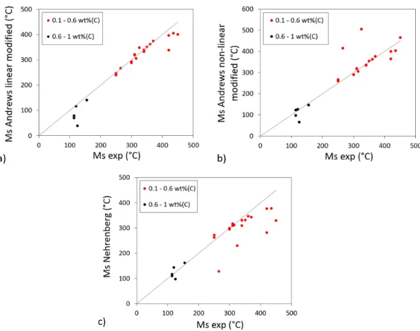
by (a) Andrews modified linear, (b) Andrews modified non‐linear and (c) Nehrenberg’s equations, for nano‐bainitic compositions found in the literature [33, 46, 48, 130, 131, 137‐144]. ... 31
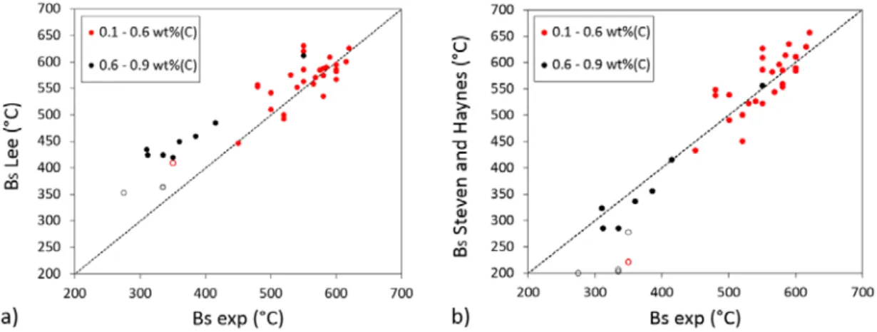
Figure 2‐21: Comparison of (a) Lee’s and (b) Steven and Hayne’s formulae for calculation of the Bs of steels with carbon contents ranging from 0.1 to 0.6 wt% and
0.6 to 0.9 wt%. Open circles correspond to alloys with a high Mn content (>3.5 wt% Mn). ... 33 Figure 2‐22: Effect of carbon content (a) on the TTT diagram C‐curve associated with the formation of 15 vol% of bainite in plain carbon steels [23], and (b) on the growth rate of bainite needles at 400 °C [45]. ... 34 Figure 2‐23: Retarding effect of silicon on (a) the lengthening rate of bainite laths in a 0.5 wt%(C) steel [116] and (b) on the bainitic isothermal transformation for the formation of 10 %, 50 % and 90 % of bainite at 250 °C in a 0.9 wt%(C) steel [137], and (c) Promoting effect of silicon on the amount of retained austenite after isothermal bainitic transformation at 250 °C [137]. ... 36 Figure 2‐24: Retarding effect of manganese on the formation of 10, 50 and 90 % of bainite in high‐carbon steels. Adapted from [137]. ... 37 Figure 2‐25: Solidification surface on the substrate side of a steel in the case of (a) a smooth substrate (ridge pitch value of zero) and (b) a rough substrate (ridge pitch of 200 μm), and effect of substrate roughness (ridge pitch) on (c) the nuclei density on the substrate side of the sample and (d) the maximum heat flux. Figures adapted from ref [166]. ... 42 Figure 2‐26: Cooling curves of an aluminium alloy associated with various casting processes. Note the logarithmic time scale. Adapted from [170]. ... 43 Figure 2‐27: Cooling rate and secondary dendrite arm spacing (SDAS) ranges associated with various casting routes. DSC refers to direct strip casting. Adapted from [2]. ... 44 Figure 2‐28: Dendritic structure highlighted by etching of strip cast specimens. Image adapted from [10, 11]. ... 46 Figure 2‐29: Particular arrangement of precipitates in the inter‐dendritic arm spaces. This figure illustrates both the presence of micro‐segregation and the shorter SDAS in strip cast materials as compared to conventionally cast products [22]. ... 47 Figure 2‐30: Recrystallization kinetics and grain size as a function of fraction
free from precipitates, and (e) 90 %‐recrystallized microstructure of alloyed denoted Fe‐0.5C in (a‐b) showing the elongated shape of recrystallized grains. Adapted from [202]. ... 50 Figure 2‐31: Banded microstructure in a hot‐rolled steel plate showing alternating layers of ferrite (bright phase) and pearlite (dark phase) due to chemical micro‐ segregation [178]. ... 52 Figure 2‐32: Banded structures in a coiled strip cast low‐carbon steel containing Nb, showing polygonal ferrite in the core of the dendrites, and pearlite in the inter‐ dendritic regions [12]. ... 53 Figure 3‐1: (a) Three‐dimensional representation of the dip‐caster used in this work with the copper substrate in the immersed position, (b) photograph of the immersion paddle, and (c‐d) photographs of the strip cast dip sample, (c) surface in contact with the copper substrate and (d) surface on the melt side. ... 58 Figure 3‐2: Cooling curve during direct strip casting, measured using a thermocouple attached to the copper substrate. ... 59 Figure 3‐3: Thermal treatments during casting of the alloys studied. For each composition, (AC) designs as‐cast samples, and (T) specimens coiled at 310 °C for 24 hours then air‐cooled to room temperature. The two cooling rates indicated correspond to the onset of solidification (‐ 103 °C/s) and the average cooling rate in
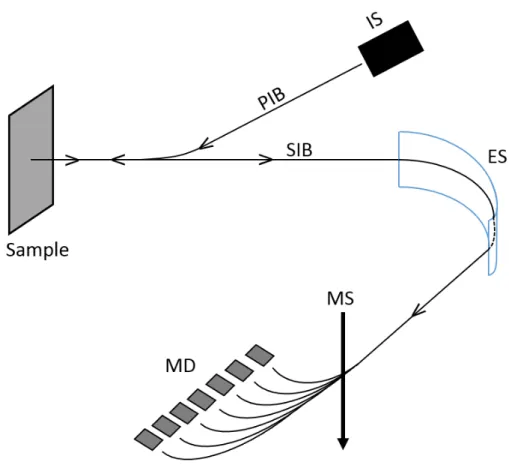
the 500 – 800 °C range (‐ 10 °C/s). ... 61 Figure 3‐4: Specimen geometry and position in the induction heating coil. Dilatometer experimental setup. ... 63 Figure 3‐5: Summary of the thermal schedule from casting to the end of the dilatometry treatments of (a) the segregated and (b) the homogenised specimens. The dilatometry segments (black) present here the isothermal treatment. ... 64 Figure 3‐6: Functional schematic of the NanoSIMS equipment used in the present work. IS: ion source; PIB: primary ion beam; SIB: secondary ion beam; ES: electrostatic sector; MS: magnetic sector; MD: multi‐detection unit. ... 67 Figure 3‐7: Atomic scattering factor of iron as a function of sin(θ)/λ, adapted from [216]. ... 71 Figure 3‐8: Comparison between the volume fractions of austenite obtained by XRD and EBSD in the coiled specimens. Black dotted unity line indicated. ... 75
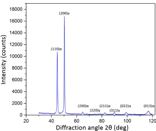
Figure 4‐1: X‐Ray Diffraction spectrum of sample 5AC, showing the presence of retained austenite and a body‐centered phase. ... 79 Figure 4‐2: Volume fractions of retained austenite in the as‐cast specimens given by X‐ray diffraction. The standard error was 5 % of the measured value. ... 80 Figure 4‐3: Optical micrographs of the cross section of the air‐cooled samples, x200. The arrow indicates the solidification direction for all specimens. ... 81 Figure 4‐4: SEM secondary‐electron images of the air‐cooled samples, showing coarse laths‐ martensite microstructures in all specimens. The arrow indicates the solidification direction for all samples. ... 82 Figure 4‐5: Volume fraction of retained austenite in the coiled specimens compared to that in the as‐cast samples, given by X‐Ray diffraction. ... 84 Figure 4‐6: Electron images showing a nano‐bainitic microstructure in all coiled specimens. Martensite lenses appear in compositions 4 and 5 (d‐e). A high magnification image shows the fine stack of bainite‐austenite laths within a bainite sheaf (f). αb: individual bainite lath, αnb: nano‐bainite (bainite laths + retained
austenite films), αM: martensite, γ: austenite. Solidification direction aligned with
vertical direction. ... 86 Figure 4‐7: EBSD images of the low‐carbon specimens 1 (a, c, e) and 2 (b, d, f) after coiling at 310 °C for 24 hours. (a, b) Band‐Contrast maps, (c, d) phase map with bainite in blue and austenite in red and (e, f) Euler angle map. Solidification direction aligned with vertical direction. ... 88 Figure 4‐8: EBSD images of sample 3T. (a) Band‐Contrast, (b) phase map with ferrite in blue and austenite in red and (c) Euler angle map. Solidification direction aligned with vertical direction. ... 89 Figure 4‐9: EBSD images of the high‐carbon‐high‐silicon specimens 4 (a, c, e) and 5 (b, d, f) after coiling at 310 °C for 24 hours. Band‐Contrast maps (a, b), phase map with bainite in blue and austenite in red (c, d) and Euler angles map (e, f). Solidification direction aligned with vertical direction. ... 91 Figure 4‐10: High‐magnification image in a bainite sheaf showing (a‐c) bainite laths separated by retained austenite films and (b‐d) associated EBSD phase map with austenite in red and ferrite in blue. ... 92
Figure 4‐11: Electron back‐scattered image of a bainite sheaf showing the presence of (a‐c) stacking faults and (d) dislocations in the austenite films adjacent to bainite laths. αb: bainite, γ: austenite. ... 93
Figure 4‐12: Misorientation angle distribution of the bainite/austenite interface in specimen 5T showing a preference for the N‐W orientation relationship. Theoretical K‐S and N‐W orientation relationships obtained from [223]. ... 94 Figure 4‐13: Lenticular martensite in sample 5T. αb: bainite, αLM: lenticular
martensite. ... 94 Figure 4‐14: Stress induced in the austenite as a results of lenticular martensite formation: (a) dislocations and stacking faults along the edge and (b) at the tip of the martensite lenses. ... 95 Figure 4‐15: Bainitic ferrite lath width distributions in the coiled specimens. ... 96 Figure 4‐16: Phase volume fractions in the specimens coiled 24 hours at 310 °C, obtained by combination of X‐Ray Diffraction (austenite) and image analysis (bainitic ferrite, martensite). ... 97 Figure 4‐17: EBSD Euler maps of the austenite in the Dip Direction (DD) – Normal Direction (ND) plane (cross‐section) of specimen 5. Substrate side of the specimen on the bottom, solidification direction along ND. ... 98 Figure 4‐18: EBSD Euler maps of the austenite in the Dip Direction (DD) ‐ Transverse Direction (TD) plane on the substrate side (left) and on the melt side (right) of sample 5T, and corresponding austenite inverse pole figures. ... 99 Figure 4‐19: Austenite grain size distributions corresponding (a) to the substrate side and (b) to the melt side of the specimen. Log‐Normal distribution of the substrate side in red. ... 100 Figure 4‐20: EDS maps of the cross‐section of sample 5AC, showing the segregation of interstitial elements (silicon, chromium and manganese) in the inter‐dendritic regions during solidification. Normal (solidification) direction aligned with vertical direction. ... 102 Figure 4‐21: Nano‐SIMS mapping of sample 5T showing the segregation of substitutional elements in the inter‐dendritic regions. ... 104
Figure 4‐22: Nano‐SIMS map and segregation quantification profile of Manganese, Silicon, Chromium and Aluminium along the green horizontal line. Profiles fitted using a Pearson VII function for Mn, Si and Cr and a Gauss function for Al. ... 105 Figure 4‐23: High magnification Carbon map obtained by nano‐SIMS and associated phase schematic: the area presents bainite sheaves (ferrite and retained austenite laths, blue in schematic), and pockets of martensite lenses (green in schematic). 107 Figure 4‐24: Sequence of image modification to account for the crystal orientation contrast in the SIMS carbon map. ... 108 Figure 4‐25: Carbon concentration profile across a bainite sheaf, measured by nano‐ SIMS. ... 109 Figure 4‐26: EBSD‐EDS correlation in sample 5AC. (a) Band contrast, (b) phase map with austenite in red and ferrite in blue, (c) IPF colouring, (d) EDS silicon K‐lines map, (e) Euler colouring, and (f) superimposition of the austenite from (b) on the silicon EDS map (d) showing the concentration of retained austenite in the segregated inter‐dendritic arms. Solidification direction aligned with vertical direction. ... 110 Figure 4‐27: Aluminium nitrides and manganese sulphides revealed by EDS. Note that (a‐b) and (c‐f) present two different regions of the sample. Solidification direction aligned with vertical direction. ... 111 Figure 4‐28: EDS merged image showing the aluminium nitrides and manganese sulphides in the enriched inter‐dendritic regions. Silicon in green, aluminium nitrides in red, manganese sulphides in yellow. Solidification direction aligned with vertical direction. ... 112 Figure 4‐29: Evolution of grain morphology during solidification, adapted from [236]. The red box highlights the morphologies found in the strip cast alloys studied in the present work. ... 114 Figure 4‐30: Angle of dendritic growth with respect to the normal (solidification) direction in specimen 5T. ... 115 Figure 4‐31: Comparison between the Scheil predictions and experimental quantifications of micro‐segregation in the alloys studied, obtained by EDS (full symbols) and nano‐SIMS (empty symbols). The line of slope 1 is also plotted to show
Figure 4‐32: Phase stability at equilibrium as a function of temperature in specimen 5, Thermocalc. ... 118 Figure 4‐33: [Al].[N] product (a) in the inter‐dendritic liquid and (b) in austenite, compared to AlN solubility in the respective phases showing that AlN are favourable across the whole solidification range. ... 120 Figure 4‐34: Liquid enrichment in Mn and S as solidification proceeds according to Scheil, Thermocalc. ... 122 Figure 4‐35: [Mn].[S] product in a) the inter‐dendritic liquid and b) in austenite, compared to MnS solubility in the respective phases. The onset of precipitation in the liquid is marked with the red dot. No precipitation is predicted in austenite. . 123 Figure 4‐36: Equilibrium calculations a) in the first and b) in the last liquid to solidify. Compositions given by Scheil calculations. MnS becomes stable in the liquid at the end of solidification, temperature range highlighted by the box in (b). ... 124 Figure 4‐37: EDS maps showing AlN and MnS precipitates. Common positions highlighted with the yellow circles. ... 125 Figure 4‐38: Solidification‐precipitation sequence in the alloys studied. Aluminium nitrides (AlN) and manganese sulphides (MnS) formed at the end of solidification in the super‐saturated liquid between the dendrites. ... 127 Figure 4‐39: Predictions of the martensite start temperature Ms in all compositions.
... 128 Figure 4‐40: Martensite volume fraction as a function of temperature during cooling, according to the Koistinen‐Marburger model with composition‐dependent parameters, (a) in the full range of martensite volume fractions and (b) limited to the martensite volume fractions above 80 vol%. The red vertical line in (a) highlights room temperature. The black vertical lines in (b) highlight for each alloy the M99
temperature, corresponding to a martensite volume fraction of 99 vol%. ... 130 Figure 4‐41: Comparison between the experimental (XRD) and predicted (Koistinen‐ Marburger model) martensite volume fractions at room temperature in all specimens. Vertical error bars within dot radii. ... 131 Figure 4‐42: Koistinen‐Marburger predictions in (a‐b) the depleted regions and (c‐d) the enriched inter‐dendritic areas of the alloys studied. (a‐c) present the full range of martensite volume fractions and (b‐d) are limited to the martensite volume
fractions above 80 vol%. The black vertical lines in (b‐d) highlight for each alloy the temperature corresponding to a martensite volume fraction of 99 vol%. ... 132 Figure 4‐43: Differences in martensite morphology showing (a) lath‐martensite in composition 2 and (b) plate‐martensite in composition 4. Solidification direction aligned with vertical direction. ... 133 Figure 4‐44: Schematic microstructure morphologies in the coiled specimens. Solidification direction aligned with vertical direction. ... 136 Figure 4‐45: Bainite lath width ‐ austenite strength correlation in the alloys studied in this work (red points) and in alloys referenced in Singh’s work [138] (black points). ... 139 Figure 5‐1: Schema of the microstructure of the strip cast specimen of composition 5 after coiling at 310 °C for 24 hours. ... 142 Figure 5‐2: Thermal treatment applied in the dilatometer. Tc refers to the coiling
temperature. ... 144 Figure 5‐3: Energy‐Dispersive‐Spectroscopy (EDS) of (a‐b) the as‐cast dip sample, (c‐ d) sample after austenitizing treatment 2 min at 1150 °C, and (e‐f) after homogenisation treatment 8 hours at 1100 °C, showing (a‐c‐e) the silicon K‐line maps and (b‐d‐f) MnS precipitates. ... 146 Figure 5‐4: EBSD images showing the prior‐austenite grain morphology in (a) the strip cast dip sample, (b) the segregated sample 5S after austenitizing treatment and (c) the homogeneous sample 5H after austenitizing treatment. The white lines correspond to the austenite grain boundaries (> 15° angles). Solidification direction along ND. ... 148 Figure 5‐5: Back‐scattered electron micrographs of (a) the strip cast dip sample, (b) segregated sample 5S and (c) homogeneous sample 5H transformed at 310 °C for 24 hours: αnb nanobainite sheaves and αLM lenticular martensite pockets. ... 149
Figure 5‐6: Bainitic ferrite lath width distribution in (a) segregated sample 5S and (b) homogeneous sample 5H transformed at 310 °C for 24 hours in the dilatometer. Raw and stereologically corrected average values are presented in the table. ... 151 Figure 5‐7: Bainite sheaves length and width in (a‐c) segregated sample 5S and (b‐d) homogeneous sample 5H transformed at 310 °C for 24 hours in the dilatometer. 152
Figure 5‐8: (a) Dilatometry response during thermal treatment. Bainite formation highlighted by red hashed region. Temperature (black curve) and length change of the sample (blue curve) as a function of time, ti incubation time for the start of
bainite transformation. (b) Graphical determination of the end of incubation. The green region in (b) highlights the uncertainty on the measurement of ti. ... 153
Figure 5‐9: Incubation time for bainite formation in the segregated (red) and the homogeneous (blue) samples. The data points were fitted by a degree 2 polynomial function. The indicated BS is that of the homogeneous sample, as calculated using
Steven and Haynes formula. ... 154 Figure 5‐10: Length change of the homogeneous dilatometry sample associated with bainite growth at 290 °C. ... 155 Figure 5‐11: Bainitic ferrite volume fraction as a function of time after the end of incubation in (a) the segregated and (b) the homogeneous samples: effect of transformation temperature. ... 159 Figure 5‐12: Bainite volume fraction as a function of time of isothermal transformation at 290 °C, 300 °C, 310 °C and 320 °C. Segregated sample in red, homogeneous sample in blue. ... 160 Figure 5‐13: Dilatometry data of the segregated sample showing (a) the formation of bainite during isothermal treatment and (b) the formation of martensite during quenching at the end of the isothermal treatment. Point Q corresponds to the onset of quenching. The green vertical line in (b) marks the onset of martensite formation during quenching. ... 161 Figure 5‐14: Selection of the area near prior‐austenite grain boundaries in the strip cast dip sample of composition 5, coiled at 310 °C for 24 hours. (a) Austenite Euler colour map, (b) corresponding schema with prior‐austenite grain numbering 1‐3, (c) EDS silicon K‐line map and (d) band contrast map of the corresponding area. ... 165 Figure 5‐15: (a) Merged map consisting of (b) the EBSD band‐contrast map and (c) the EDS silicon map of the dip sample of composition 5 coiled at 310 °C for 24 hours. The white dotted‐lines correspond to prior austenite grain boundaries, the yellow ellipses highlight the enriched regions where bainite did not form. ... 166 Figure 5‐16: (a) Nano‐SIMS Mn map in the strip cast dip specimen showing the line (AB) along which (b) the driving force for ferrite nucleation and (c) the bainite start
temperature were calculated using Thermocalc and Steven and Haynes’ formula respectively. The driving force for ferrite nucleation and the Bs in the homogeneous
specimen (blue dotted‐lines in (b) and (c)) and the coiling temperature (black TC line
in (c)) are indicated. ... 167 Figure 5‐17: Effect of the undercooling (a) below T0 and (b) below BS on the
maximum bainite volume fraction. Red points and blue points correspond to the heterogeneous and homogeneous specimens respectively. The composition of the segregated sample is that in the solute‐depleted regions, where the bainite laths formed. ... 169 Figure 5‐18: Global kinetics of bainite transformation in the range 290 °C ‐ 320 °C in the segregated (red) and homogeneous (blue) samples. dX/dt first derivative of bainite volume fraction with respect to time, here presented as a function of the bainite volume fraction. ... 172 Figure 5‐19: Effect of temperature on the maximum bainite transformation rate in the segregated (red) and the homogeneous (blue) samples. ... 173 Figure 5‐20: Effect of the undercooling (a) below T0 and (b) below BS on the
maximum bainite transformation rate. Red points correspond to the segregated sample, blue points to the homogeneous specimen. The composition of the segregated sample is that in the solute‐depleted regions... 174 Figure 5‐21: Interrupted treatment at 310 °C to measure the bainite spatial nucleation rate in (a) the segregated and (b) the homogeneous specimens. Note the scale difference between (a) and (b). The transformation times indicated refer to the time after the end of incubation in each specimen. ... 175 Figure 5‐22: Bainite lengthening rate in the depleted (red squares) and enriched (red triangles) areas of the segregated sample and in the homogeneous specimen (blue squares), calculated as per method described in [116]. ... 179 Figure 6‐1: Thermal treatment applied in the dilatometer prior to cooling at controlled rates. ... 186 Figure 6‐2: Continuous‐Cooling‐Transformation (CCT) diagrams of the homogeneous specimens, compositions 1H to 5H (respectively a‐e). Ae1, Ae3 and Acm temperatures
Figure 6‐3: Phases formed during continuous cooling of specimen 1H: (a) full pearlite, (b) mixture of bainite and martensite) and (c) full martensite. Backscattered electrons signal. ... 189 Figure 6‐4: Pearlite nose position on the CCT diagram of the homogeneous samples. The element which concentration varies between two consecutive samples is indicated. ... 191 Figure 6‐5: Continuous‐Cooling‐Transformation (CCT) diagrams of the segregated strip cast specimens of compositions 1‐5 (respectively a‐e). The black dashed line on each graph presents the cooling curve measured by a thermocouple during the actual direct strip casting process. Ae1, Ae3 and Acm temperatures indicated. Error
bars within points radii. Cooling rates indicated on some cooling curves. ... 193 Figure 6‐6: Comparison of the experimental Ms in the homogeneous (blue) and
segregated (red) specimens of each bulk composition. Experimental error +/‐ 5 °C. ... 194 Figure 6‐7: Pearlite nose position comparison between homogeneous and segregated specimens of each composition. ... 196 Figure 6‐8: CCT diagram of specimen 5S limited to the pearlite transformation. The cooling curve corresponding to a cooling rate of ‐1 °C/s is highlighted in blue. PS and
Pf refer to the pearlite start and finish temperatures, and t the time for pearlite
completion at the considered cooling rate. ... 199 Figure 6‐9: Diffusion distance of the various elements during pearlite formation at the start and finish temperatures in specimen 5S cooled down at ‐1 °C/s. ... 200 Figure 6‐10: Dilatation curves of the segregated samples 1‐5 (a‐e) showing the martensite phase transformation at ‐10 °C/s cooling rate. ... 204 Figure 6‐11: Theoretical MS comparison between homogeneous and segregated
specimens of each composition. ... 206 Figure 6‐12: Comparison between calculated and experimental martensite start temperatures in the homogeneous (blue) and the segregated (red) samples. Error on the experimental MS +/‐ 5 °C. ... 207
Figure 6‐13: Merged CCT diagrams of alloys 1 to 5 (a‐e) in the homogeneous (full lines) and segregated (dotted lines) conditions. ... 208
Figure 6‐14: Pearlite nucleation (a‐c‐e) in specimen 2S cooled at ‐2 °C/s and (b‐d) in sample 2H cooled at ‐1 °C/s. Microstructures consisting of pearlite (dark) and martensite (grey). Bainite laths can also be seen in sample 2H. (e) Silicon K‐line EDS map corresponding to image (c). ... 210 Figure 6‐15: Experimental pearlite start temperature measured on the CCT diagrams at a cooling rate of ‐0.5 °C/s, as a function of the calculated Ae1 temperature. The
latter are presented in the homogeneous samples (blue squares), and in the depleted regions of the segregated specimens (red squares). ... 212 Figure 6‐16: Merged CCT diagrams of composition 1 in the homogeneous (full lines) and segregated (dotted lines) configurations. ... 214 Figure 6‐17: Merged bainite curves (CCT diagrams) of alloy 2 in the homogeneous (full lines) and segregated (dotted lines) configurations. ... 216
List
of
tables
Table 2‐1: Stabilising properties of the classical alloying elements used in steelmaking, adapted from [36]. ... 6 Table 2‐2: Average error associated with the various MS prediction formulae,
calculated from the data presented in Figure 2‐20. ... 31 Table 2‐3: Average error associated with the various BS prediction formulae,
calculated from the data presented in Figure 2‐21. ... 33 Table 2‐4: Selected formulae for Ms and Bs calculations. ... 34
Table 3‐1: Nano‐bainitic compositions (in wt%) selected for the present project. The predicted MS and BS are indicated. ... 56
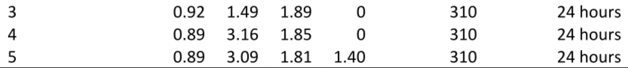
Table 3‐2: Summary of the selected alloys, coiling temperature (Tc) and time (tc).
Compositions are in wt%. ... 60 Table 4‐1: Quantitative Energy‐Dispersive‐Spectroscopy analysis of the specimens studied. Concentrations are given in wt%. ... 103 Table 4‐2: Comparison of the segregation quantification by EDS and Nano‐SIMS in specimen 5T, showing the good agreement between the two techniques. Concentrations are given in wt%. ... 106 Table 4‐3: Volume fraction of sample above and below bulk composition due to micro‐segregation in specimen 5T, determined from Nano‐SIMS image analysis. . 106 Table 4‐4: Concentration range (Min ‐ Max) in each specimen, as calculated by Thermocalc using Scheil conditions of solidification. ... 116 Table 4‐5: Predicted Ms of the austenite laths and the austenite blocky regions.
Carbon concentrations obtained by Nano‐SIMS, Ms predicted using Nehrenberg's
formula. ... 134 Table 4‐6: Estimation of austenite strength at 310 °C in all alloys. Calculated using equation given in [138]. Compositions are given in wt%, strength in MPa. ... 138 Table 5‐1: Compositions (in wt%) and transformation temperatures in the homogeneous and segregated (depleted and enriched regions) alloys of composition 5. The number in red corresponds to a BS value out of the composition
Table 5‐2: Summary of the microstructural features in the 3 samples compared in the present chapter: strip cast dip specimen, segregated dilatometry sample 5S, and homogeneous dilatometry sample 5H. ... 162 Table 5‐3: Bainite lath thickness and austenite strength at 310 °C in the depleted areas of the segregated sample and in the homogeneous specimen. ... 163 Table 5‐4: Parameters for bainite lengthening rate calculations. ... 178 Table 5‐5: Alloy concentration in the depleted areas of the segregated sample according to Nano‐SIMS, MS of the segregated sample obtained by dilatometry after
treatment at 310 °C (MS dilatometry), Carbon concentration of the martensite pockets
deducted from MS dilatometry (Cdilatometry) and obtained by Nano‐SIMS (CNano‐SIMS).
Compositions are given in wt%. ... 182 Table 6‐1: Martensite start temperature Ms of the homogeneous alloys determined
experimentally by quenching dilatometry, and theoretical values determined with Andrews’ (compositions 1 ‐ 2) and Nehrenberg’s formulae (compositions 3 – 5). . 190 Table 6‐2: Eutectoid temperature Ae1 in the homogeneous specimens, calculated
using Andrews formula [136]. ... 192 Table 6‐3: Martensite start temperature Ms of the segregated alloys, determined
experimentally by quenching dilatometry. ... 194 Table 6‐4: Eutectoid temperature Ae1 in the homogeneous samples, and in the
enriched and depleted regions of the segregated samples. ... 197 Table 6‐5: Diffusion coefficients used for calculations. ... 199 Table 6‐6: Summary of the effect of carbon, silicon and chromium on phase transformations during continuous cooling. The text in red highlights the discrepancies with the literature. ... 202
Chapter
1.
Introduction
Direct strip casting (DSC) is a new process for the production of thin steel sheets from the melt in a single step [1]. By eliminating the numerous secondary thermomechanical steps needed after conventional casting methods, DSC allows significant energy, time and cost savings [2]. Materials produced by DSC undergo extremely high solidification and cooling rates in the order 103 °C/s at the onset of
solidification [2, 3]. In such conditions, non‐equilibrium microstructures form. Non‐ equilibrium concentrations of alloying elements in solid solution [4‐7], refined precipitates [5, 8, 9], and short‐wavelength micro‐segregation of impurities [10, 11] are examples of the features inherited from DSC which are not emulated in slow cooled slab castings. Such features were shown to have a significant impact on the morphology of the microstructures developing during secondary processes such as static recrystallisation [12, 13]. However, the effect of micro‐segregation on the kinetics of phase transformations has not before been studied.
Nano‐bainitic steels received extensive attention in the past decades due to the remarkable mechanical properties they exhibit. These alloys of simple chemistry present high strength levels while retaining toughness in the excess of 40 MPa.m1/2
[14‐16]. Though these unique microstructures have been extensively studied in conventional steels, they have never before been investigated in alloys produced by direct strip casting.
This thesis examines the impact of the particular features inherited from direct strip casting on microstructure development in 5 medium to high carbon steels designed for nano‐bainite development. In particular, the impact of the solidified grain structure, fine precipitation, and micro‐segregation of substitutional elements that develop during DSC on the morphology and kinetics of phase transformations during continuous cooling and isothermal treatment are investigated.
Chapter
2.
Literature
Review
2.1.
Direct Strip Casting
Direct strip casting (DSC) is a near‐net shape casting method in which molten steel is poured directly on counter‐rotating copper rolls to achieve the final product, as illustrated in Figure 2‐1.
Figure 2‐1: Three‐dimensional representation of Bessemer's strip caster, adapted from [2].
Solidification of the molten steel occurs upon contact with the cold copper rolls, followed by dendritic growth into the liquid, Figure 2‐2. At the nip point of the rolls the two solidifying shells on each roll connect to form a single steel strip [2, 17]. Despite being a fairly old concept [2], DSC has only recently been brought to industrial production [1].
Figure 2‐2: Steel strip formation at the nip point during twin‐roll strip casting, adapted from [2].
Because DSC is a near‐net shape process, the thickness of the steel sheet after solidification is close to that of the final product. This allows the elimination of many secondary processing steps such as hot and intermediate rolling [18], thus resulting in a decrease in the overall processing costs, a decrease in the plant dimensions and significant energy savings: it was estimated that the production of steel sheets through DSC instead of conventional casting would allow a reduction in the energy consumption by more than 85 % [19, 20]. The economic and environmental advantages of this process are therefore clear. Figure 2‐3 illustrates the significant reduction in plant size that comes with a production by DSC instead of conventional slab casting.
Figure 2‐3: Dimension differences between conventional slab casting and direct strip casting. The latter allows significant reduction in plant size and production costs for thin sheets. Figure adapted from [4].
However, the radical change in processing has a significant impact on the subsequent microstructural development. Strip cast microstructures are strongly affected by the non‐equilibrium rapid cooling conditions experienced during solidification and subsequent phase transformations [2, 21]. For the case of a low‐ carbon steel, it has been shown that the final microstructure of a steel produced by conventional slab casting is markedly different to that produced by DSC. Figure 2‐4 shows that the fine equiaxed ferrite microstructure of steel produced by conventional casting can be changed to a more complex microstructure consisting of coarse Widmanstätten ferrite and polygonal ferrite in the same alloy produced by DSC. Such differences arise from the significant morphological difference in the solidification structure between the two processes [2, 13, 21], in addition to the markedly reduced thermo‐mechanical processing window available after DSC.
Figure 2‐4: Comparison between (a) the microstructure of a steel produced by direct strip casting (CASTRIP process) showing coarse Widmanstätten and polygonal ferrite, and (b) that of the same steel produced by conventional slab casting showing fine equiaxed ferrite grains [21].
Minor changes in compositions have been shown to induce major changes in microstructures in DSC steels. For instance, slight additions of vanadium to a low‐ alloy steel chemistry can turn a blocky ferrite microstructure into a fully bainitic one under DSC conditions [22]. The behaviour of the different elements such as carbon, silicon, manganese, chromium is therefore different during DSC as compared to conventional casting. Solute behaviour under conventional processing conditions has been extensively studied [23, 24], however, the behaviour of different solutes under strip cast conditions remains unclear and is still under investigation [2]. To date, DSC studies have mainly investigated plain carbon steels, and more recently Nb‐micro‐alloyed steels have been studied [25‐33]. In particular, it was shown that the high cooling rates experienced during DSC prevent precipitation and lead to super‐saturated solid solutions. These properties were successfully exploited in Nb‐steels where reheating led to considerable strengthening by cluster formation and better mechanical properties than in conventionally cast materials [30]. This demonstrates that DSC offers the opportunity to produce new microstructures with potentially improved properties compared to conventional casting. It is therefore of great benefit to re‐assess what microstructures are to be expected in strip cast materials as compared to conventionally cast materials.
2.2.
Phase Transformations in Steels
Steels produce an extensive range of mechanical properties [34] related to the existence of different allotropes (forms) for iron [35, 36]. Transitions between these various forms are called phase transformations and the latter govern microstructural development in steels. These transitions are described in the following sections.
2.2.1. Effect of Alloying Elements
Various elements can be added to steels in order to control their microstructure and physical properties. These alloying elements can be classified into two categories depending on their thermodynamic effect on the phase diagram, ferrite stabilisers and austenite stabilisers. Table 2‐1 summarizes the effect of the classical alloying elements used in the steel industry.
Table 2‐1: Stabilising properties of the classical alloying elements used in steelmaking, adapted from [36].
Alloying elements α ‐ stabilisers Si Cr Al P B V W Ta Nb Zr Ti Mo γ ‐ stabilisers C Mn N Cu Ni Co The austenite stabilisers and ferrite stabilisers respectively expand and contract the austenite phase field of the phase diagram. These changes occur by moving the Ae1,
Ae3, and Acm temperatures as well as the eutectoid composition, as shown in
Figure 2‐5. As can be seen, the austenite stabilisers (Ni, Mn) depress the eutectoid temperature Ae1 while the ferrite stabilisers increase it. Aside from these
modifications, alloying elements can form stable compounds such as carbides, nitrides and sulphides (MnS, AlN, Cr23C6, TiC, Al4C, NbN) which adds further
complexity the Fe‐C phase diagram.
Figure 2‐5: Effect of various alloying elements on the eutectoid temperature and composition [37].
2.2.2. The Limitations of the Phase Diagram: Non‐Equilibrium Phases
Phase diagrams are an effective tool to predict the formation of equilibrium phases obtained by transformations at infinitely slow cooling rates. Their use is therefore limited when trying to predict the microstructures obtained in complex alloys produced in industrial conditions at various cooling rates. The steel phase diagram suggests that the only phases which can be observed at room temperature are ferrite, cementite and eutectoid pearlite. This diagram does not account for the formation of transformation products such as martensite or bainite.
2.2.3. Transformation Kinetics and Cooling Rate
The kinetics of transformation and the applied cooling rate are critical parameters that determine the formation of microstructures not predicted by thermodynamics and the equilibrium phase diagram, such as retained austenite at room temperature, martensite or bainite. Since equilibrium phase diagrams do not account for transformation kinetics, they are ineffective in predicting the formation of non‐equilibrium phases. Instead, time‐temperature diagrams are used in this regard. Two types of diagrams are widely used: time‐temperature‐transformation (TTT) diagrams and continuous‐cooling‐transformation (CCT) diagrams. Both diagrams are typically obtained by dilatometry [38‐44].
2.2.3.1. Time‐Temperature‐Transformation (TTT) Diagrams
Time‐Temperature‐Transformation (TTT) diagrams map the occurrence areas of both the equilibrium and non‐equilibrium phases which develop in an alloy during isothermal treatment. The advantage of TTT diagrams as compared to equilibrium phase diagrams is that they incorporate time which is a critical parameter in understanding metastable phase transformations in steels. Each diagram is associated with one particular chemical composition [24], and an example is shown in Figure 2‐6.
Figure 2‐6: TTT‐diagram of a medium‐alloyed steel, showing the C‐curves associated with pearlite (P) and bainite (B), adapted from [24].
The curves drawn in a TTT‐diagram usually have a C‐shape [24]. The C‐shape can be explained by understanding that diffusional phase transformation kinetics are mostly dependent on two parameters, the driving force for the reaction ∆ , and the diffusivity of the considered species. The higher these two parameters are, the faster the phase transformation. ∆ and D are strongly dependent on the temperature T at which the system is held. There are two regimes to consider:
At high temperatures, the diffusion coefficient D is large, but the undercooling is small, thus the driving force for the transformation ∆ is small.
At low temperatures, the diffusivity is reduced while the undercooling and hence the driving force for the reaction are increased.
In these two extreme cases, the time to complete transformation is large. For intermediate temperatures, a better compromise between the values of ∆ and D allows the transformation to be completed faster, hence the C‐shape of the curves.
However, the addition of certain alloying elements such as the carbide‐formers Mn, Cr, Mo, W, V, Ti, Zr, Nb [37] can distort these curves and lead to more complicated shapes [24].
2.2.3.2. Continuous‐Cooling‐Transformation (CCT) Diagrams
Continuous‐Cooling‐Transformation diagrams (CCT‐diagrams) are the second type of widely used diagrams in predictive metallurgy. They differ from the TTT‐diagrams in that they are obtained through continuous cooling of the samples instead of isothermal holding. They are therefore useful in predicting microstructural changes under industrial conditions such as casting. The onset points of a given phase transformation at each cooling rate are plotted in a time‐temperature diagram and linked together. The line interpolates the boundary for the region of formation of the considered phase. Figure 2‐7 shows an example of a CCT diagram. It can be seen that austenite, bainite and martensite all appear on this diagram. The phase fields in CCT diagrams do not necessarily have a C‐shape. The complexity of the shapes is mainly due to the fact that during continuous cooling, different phases may form at different temperatures, and this sequence of events may alter the subsequent transformation behaviour.
Figure 2‐7: CCT‐diagram showing the occurrence areas of the different phases that can be formed under continuous cooling conditions in a HSLA steel. The cooling curves were plotted as well [24].
The austenite/martensite boundary (dotted‐line in Figure 2‐7) is horizontal, and corresponds to the martensite start temperature Ms. This temperature is not
kinetic, and does not depend on the cooling rate provided no other phase forms upon cooling prior to martensite formation. However it strongly depends on the austenite chemistry, in particular austenite carbon concentration as discussed in 2.3.1. It is therefore influenced by the presence of other phase transformations: for a given cooling rate, the Ms can be gradually depressed (respectively increased) if
martensite formation is preceded by the formation of a phase accommodating less (respectively more) carbon than the overall alloy content. The case of Ms depression
when bainite formation precedes that of martensite is illustrated by the dotted‐line in Figure 2‐7.
Apart from martensite, the upper boundary of the first phase to form upon cooling is generally not a straight line. This particularly applies to phases formed by purely diffusional processes such as polygonal ferrite and pearlite for which the undercooling is a function of cooling rate: the lower the cooling rate, the lower the undercooling at the start of transformation. Thus for ferrite and pearlite, as the
cooling rate is decreased, the fields upper boundaries on the CCT diagram (these boundaries are referred to as Ar3 and Ar1 respectively) converge to the equilibrium
temperatures Ae3 and Ae1 respectively. The lower boundaries of these phases
follow the same trend [24]. Figure 2‐8 shows the TTT and the CCT diagrams associated to a low‐alloy steel [24]. As can be seen, the two diagrams are markedly different since the formation region of a given phase is different in the two diagrams. Therefore the associated CCT and TTT diagrams of a given steel should not be compared [24, 45].
Figure 2‐8: Comparison between the TTT and CCT diagrams of a low‐alloy steel [24].
2.2.3.3. Effect of Alloying Elements on Time‐Temperature Diagrams
For most of the classically used elements, increasing the alloy concentration delays the austenite decomposition, shifting the phase fields towards longer times and/or towards lower temperatures on the Time‐Temperature diagram [24]. An exception exists for cobalt and aluminium [46], which increase both the nucleation and growth rates of pearlite [47] and low‐temperature bainite [48] by increasing the free energy change of the reaction [49]. Therefore these elements result in a shift of the pearlite and bainite stability regions to the left of the Time‐Temperature
The effect of most alloying elements on the martensite transformation are well established and documented in the literature, and are summarized in the numerous empirical formulas for Ms predictions in steels [50], which are discussed in further
detail in section 2.3.1. According to these, most alloying elements (C, N, Mn, Cr) contribute to a drop in the Ms, carbon and nitrogen having the most significant
effect. The case of silicon is generally more complex and, even though it is commonly reported to drop the Ms, it has also been shown to increase the Ms in
some alloys [50].
The impact of alloying elements on the kinetics of pearlite formation has been extensively studied [47, 51‐57]. Most of these studies come down to the partitioning/non‐partitioning of substitutional elements during pearlite formation. Substitutional elements either partition to ferrite or cementite: silicon partitions to ferrite [58] while carbide forming elements, in particular manganese [51, 59, 60] and chromium [51, 61‐63] partition to cementite during pearlite formation. Because of this partitioning behaviour, the pearlite transformation rate is thought to be controlled by the rate of partitioning of the substitutional elements, rather than carbon diffusion. Therefore increasing the concentration of substitutional elements tends to delay the kinetics of pearlite formation. This generally stands true for manganese and chromium [47]. Silicon partitions preferentially to ferrite during pearlite formation, and tends to delay cementite precipitation at low temperatures [64‐66]. However, its diffusivity in ferrite and cementite has been shown to be higher than other substitutional elements [58], therefore silicon is not believed to have a significant influence on the kinetics of pearlite formation. Finally, pearlite transformation largely relies on carbon diffusion in the austenite [54]. At any given temperature, carbon diffusivity in austenite increases as a function of carbon concentration [67]. Therefore higher carbon concentrations increase pearlite growth rate. Moreover, the driving force for cementite precipitation largely increases with increasing carbon concentrations [68], therefore the overall pearlite transformation is fostered by higher carbon concentrations. The effects of selected individual alloying elements on the bainitic transformation are further discussed in section 2.4.
2.2.4. Different Ferrite Morphologies
Austenite decomposition can produce a variety of ferrite morphologies depending on the alloy chemistry and the cooling rate. These morphologies have been classified by Dubé [69] and the classification matrix further modified by Aaronson [70], Figure 2‐9.
Figure 2‐9: Dubé morphological classification of ferrite, modified by Aaronson: (a) grain boundary allotriomorphs, (b) Widmanstätten sideplates or needles, (c) Widmanstätten sawteeth, (d) idiomorphs, (e) intragranular Widmanstätten and (f) massive structures. Adapted from [23].
In this section, these morphologies will be grouped into two categories: polygonal ferrite (idiomorphs and allotriomorphs) and plate‐like structures. The complex bainitic ferrite will be described in its own subsequent section. Martensite is dedicated its own sub‐section, but is only briefly reviewed here.
2.2.4.1. Polygonal Ferrite
Polygonal ferrite is the simplest ferritic morphology encountered in steels, formed from the austenite at relatively high temperature close to Ae3, or during continuous
![Figure 2‐2: Steel strip formation at the nip point during twin‐roll strip casting, adapted from [2].](https://thumb-us.123doks.com/thumbv2/123dok_us/1402903.2687802/29.892.332.658.160.541/figure-steel-strip-formation-point-strip-casting-adapted.webp)
![Figure 2‐5: Effect of various alloying elements on the eutectoid temperature and composition [37].](https://thumb-us.123doks.com/thumbv2/123dok_us/1402903.2687802/33.892.304.697.105.682/figure-effect-various-alloying-elements-eutectoid-temperature-composition.webp)
![Figure 2‐10: Optical micrograph (x500) of a British Standard 3100 normalized medium carbon steel etched in 3 % Nital, showing coarse polygonal ferrite (white phase) and pearlite (dark phase) [72].](https://thumb-us.123doks.com/thumbv2/123dok_us/1402903.2687802/41.892.361.638.493.772/figure-optical-micrograph-british-standard-normalized-polygonal-pearlite.webp)
![Figure 2‐14: TEM micrograph of a bainite sheaf consisting of carbide‐free bainitic ferrite nano‐laths (α, bright phase) separated by thin films of retained austenite (γ, dark phase) [128].](https://thumb-us.123doks.com/thumbv2/123dok_us/1402903.2687802/50.892.305.691.107.380/figure-micrograph-bainite-consisting-bainitic-separated-retained-austenite.webp)
![Figure 2‐26: Cooling curves of an aluminium alloy associated with various casting processes. Note the logarithmic time scale. Adapted from [170].](https://thumb-us.123doks.com/thumbv2/123dok_us/1402903.2687802/69.892.290.708.337.752/figure-cooling-aluminium-associated-various-processes-logarithmic-adapted.webp)