Scheduling in Mapreduce Clusters

DigitalCommons@University of Nebraska - Lincoln

Dissertations, and Student Research Computer Science and Engineering, Department of

2-2018

Scheduling in Mapreduce Clusters

University of Nebraska-Lincoln, [email protected]

Follow this and additional works at:https://digitalcommons.unl.edu/computerscidiss Part of theComputer Engineering Commons, and theComputer Sciences Commons

This Article is brought to you for free and open access by the Computer Science and Engineering, Department of at DigitalCommons@University of Nebraska - Lincoln. It has been accepted for inclusion in Computer Science and Engineering: Theses, Dissertations, and Student Research by an authorized administrator of DigitalCommons@University of Nebraska - Lincoln.

He, Chen, "Scheduling in Mapreduce Clusters" (2018).Computer Science and Engineering: Theses, Dissertations, and Student Research. 148.

by

Chen He

A DISSERTATION

Presented to the Faculty of

The Graduate College at the University of Nebraska In Partial Fulfillment of Requirements

For the Degree of Doctor of Philosophy

Major: Computer Science

Under the Supervision of Professors Ying Lu and David Swanson Lincoln, Nebraska

Chen He, Ph.D. University of Nebraska, 2018 Advisers: Ying Lu and David Swanson

MapReduce is a framework proposed by Google for processing huge amounts of data in a distributed environment. The simplicity of the programming model and the fault-tolerance feature of the framework make it very popular in Big Data processing.

As MapReduce clusters get popular, their scheduling becomes increasingly important. On one hand, many MapReduce applications have high performance requirements, for example, on response time and/or throughput. On the other hand, with the increasing size of MapReduce clusters, the energy-efficient scheduling of MapReduce clusters becomes inevitable. These scheduling challenges, however, have not been systematically studied.

The objective of this dissertation is to provide MapReduce applications with low cost and energy consumption through the development of scheduling theory and algorithms, energy models, and energy-aware resource management. In particu-lar, we will investigate energy-efficient scheduling in hybrid CPU-GPU MapReduce clusters. This research work is expected to have a breakthrough in Big Data pro-cessing, particularly in providing green computing to Big Data applications such 


detection. The tools we propose to develop are expected to increase utilization and reduce energy consumption for MapReduce clusters. In this PhD dissertation, we propose to address the aforementioned challenges by investigating and developing 1) a match-making scheduling algorithm for improving the data locality of Reduce applications, 2) a real-time scheduling algorithm for heterogeneous Reduce clusters, and 3) an energy-efficient scheduler for hybrid CPU-GPU Map-Reduce cluster.


Grant Information

This Ph.D. dissertation is supported by the National Science Foundation Award: 1018467, "CSR: Small: Energy Management for Heterogeneous MapReduce Data Cen-ter.


Table of Contents

CHAPTER 1. INTRODUCTION ...1

2.1 Hadoop MapReduce ...6

2.1.1 Task Scheduling & Data Locality ...8

2.1.2 Speculative Execution ...9

2.1.3 Fault Tolerance ...10

2.1.4 YARN ...10

2.2 Hadoop Distributed File System ...13

2.2.1 HDFS Architecture ...13

2.2.2 Data Placement and Fault-tolerance ...14

2.2.3 Data Balancer ...15

2.4 GPGPU and CUDA ...15

CHAPTER 3. RELATED WORK ...20

3.1 MapReduce Scheduling ...20

3.2 Power Management in Hadoop Cluster ...25

CHAPTER 4. MATCHMAKING SCHEDULER ...28

4.1 Hadoop Default FIFO Scheduler ...29

4.2 Delay Scheduling Algorithm ...30

4.3 Matchmaking Scheduling Algorithm ...31

4.4 Evaluation of Different Data Locality Policies ...35

4.4.1 Experimental Environment ...35

4.4.2 Experiments ...38

CHAPTER 5. REAL-TIME MAPREDUCE SCHEDULER ...48

5.1 Deadline Constraint Scheduler ...48

5.2 RTMR Scheduler ...50

5.2.1 Algorithm ...51

5.2.2 Proof of Correctness ...63

5.3 Evaluation of RTMR scheduler and Deadline Constraint Scheduler 72 5.3.1 Experimental Environment ...73

CHAPTER 6. ENERGY EFFICIENT SCHEDULER ...79

6.1.3 Adaptive Execution ...82

6.1.4 Relevant Container ...84

6.2 Scheduling Algorithm ...85

6.2.1 Level I: Application Scheduler ...87

6.2.2 Level II: Task Scheduler ...92

6.3 Evaluation ...93

6.3.1. Workload ...95

6.3.2. Energy Efficiency Profiling ...96

6.3.3. Experiment Results ...98

CHAPTER 7. CONCLUSION AND FUTURE WORK ...107

List of Figures

Figure 2.1 MapReduce Framework ...6

Figure 2.2 YARN Architecture[2] ...11

Figure 2.3 HDFS Architecture [2] ...14

Figure 2.4 CPU + GPU Architecture ...18

Figure 4.1 Loadgen Workload: Data Locality Ratio ...40

Figure 4.2 Wordcount Workload: Data Locality Ratio ...40

Figure 4.3 Loadgen Workload: Map Tasks' Average Response Time ...41

Figure 4.4 Wordcount Workload: MapTasks' Average Response Time ...42

Figure 4.5 Fair Scheduler: Data Locality Rate ...45

Figure 4.6 Fair Scheduler: Map Tasks' Average Response Time ...47

Figure 6.1. Turnaround time, data locality, and energy consumption for three sched-ulers ...100

List of Tables

Table 4.1 Matchmaking Algorithm ...34

Table 4.2 Locality Marker Maintenance ...35

Table 4.3 Experimental Environment ...35

Table 4.4 Facebook Workload ...38

Table 5.1 Admission Controller ...56

Table 5.2 Dispatcher Algorithm ...60

Table 5.3 Feedback Controller Algorithm ...63

Table 5.4 Experimental Environment ...73

Table 5.5 Workload I ...74

Table 5.6 Workload I’s Configuration (in Terms of Number of Map, Reduce Tasks and Deadline) ...74

Table 5.7 Workload II ...75

Table 5.8 Scheduler Performance with workload I ...77

Table 5.9 Scheduler Performance with Workload II ...77

Table 6.1 Adaptive Execution for MapReduce Application ...84

Table 6.2 Application Scheduler with Adaptive Execution ...90

Table 6.3 Application Scheduler without Adaptive Execution ...91

Table 6.4 Task Scheduler: Dispatcher ...93

Table 6.5 Experimental Environment ...94

Table 6.6 Workload I [20] ...95

Table 6.7 Workload Configuration (in terms of number of map and reduce) ...96

Table 6.8 Energy consumption of MD simulation job (1 map) on different types of nodes (1800 seconds sampling interval) ...97

Table 6.9 Energy efficiency factor for MD simulation ...97

Table 6.10 Energy efficiency factor for loadgen ...98

Table 6.11 EFH schedulers without Adaptive Execution comparing with FIFO scheduler ...101

Table 6.12 EFH schedulers with and without adaptive execution ...102

Table 6. 14 Confidence intervals with 95% confidence ...105 Table 6. 15 Standard Error Estimation ...106

CHAPTER 1. INTRODUCTION

MapReduce is a framework developed by Google [1] for processing huge amounts of data in distributed computer systems. Hadoop MapReduce [2] is the open source clone of Google’s MapReduce. Due to the simplicity of the programming model and the run-time tolerance for node failures, MapReduce is widely used as a platform to solve Big Data problems. In the following part of this dissertation, we will use Hadoop and MapReduce interchangeably.

Big Data was first used in 1970 on atmospheric and oceanic soundings [3]. People use it to refer to a collection of data sets that is too large and complex to be processed by tra-ditional tools. Examples of Big Data include social network logs, financial fraud detec-tions [4,5], AI applicadetec-tions [6,7], and electronic books. The McKinsey Global Institute reports that Big Data will “become a basis of competition, underpinning new waves of productivity growth, innovation, and consumer surplus.” With the help of MapReduce, scientists and engineers made significant progresses in many fields. For example, Michael C. Schatz [8] introduced MapReduce to parallelize BLAST that is a DNA se-quence alignment program and achieved 250 times speedup. Event logs from Facebook’s website are imported into a Hadoop cluster every hour, where they are used for a variety of applications, including analyzing usage patterns to improve site design, detecting spam, data mining and ad optimization [9]. Uber uses MapReduce to analyze mobile tra-jectory of taxi [10].

The current MapReduce scheduling, however, has some limitations.

First of all, in a MapReduce cluster, data is distributed to individual nodes and stored in their disks. To execute a map task on a node, we first need to have its input data avail-able on that node. Since transferring data from one node to another takes time and delays task execution, an efficient MapReduce scheduler must avoid unnecessary data transmis-sion. MapReduce default First In First Out (FIFO) scheduler has a policy to improve task data locality. However, it has inevitable deficiencies because of its strict FIFO service policy. Zaharia et al. [9] have developed a delay algorithm to improve the data locality rate. With their technique, a MapReduce scheduler breaks the strict FIFO job order when assigning map tasks to a node. That is, if the first job does not have a map task whose in-put data is stored in the node's disk (a so-called local task), the scheduler can delay it and assign another job’s local map tasks. A maximum delay time D is specified. Only when a job has been delayed for more than D time units will the scheduler assign the job’s non-local map tasks. For the delay algorithm, the maximum delay time D is a critical parame-ter. It is configurable but may need to vary for different workloads and hardware envi-ronments.

Secondly, many MapReduce applications [6,7], like online data analytics for spam de-tection and advertisement optimization, are time sensitive. They require real-time data processing. Scheduling real-time applications in MapReduce environment has become a significant problem. Polo et al. [11] developed a soft real-time scheduler that allows per-formance-driven management of MapReduce jobs. Dong et al. [12] extended the work by

Polo et al., where a two-level MapReduce scheduler was developed to handle a mixture of soft real-time and non-real-time jobs according to their respective performance de-mands. Although taking MapReduce jobs’ QoS (Quality of Service) into consideration, most existing approaches [11-16] do not provide deadline guarantees for the jobs. Kc and Anyan Wu were the first to investigate the hard real-time scheduling of MapReduce ap-plications [17], where they developed a Deadline Constraint scheduler, aiming to provide time guarantees for MapReduce jobs. However, the Deadline Constraint scheduler has several deficiencies (please see Chapter 5 for details), which may lead to not only re-source underutilization but also deadline violations.

Thirdly, with the increasing demands of computational power in big data analysis, Hadoop cluster becomes larger and larger (with thousands of servers) and the cost rises correspondingly. To satisfy the increasing computation power requirement with sustaable costs, General Purpose Graphics Processing Units (GPGPU or simply GPU) are in-troduced into MapReduce clusters as accelerators. Figure 1.1 provides a performance comparison between CPU and GPU clusters in running the same benchmark. A medium-size hybrid CPU-GPU cluster can be more than 3 times faster than a regular CPU cluster running Hadoop MapReduce applications but with only 1/10 of the hardware costs and 1/20 of the power consumption costs [18]. J. A. Stuart et al. [19,20] built GPMR, an im-plementation of MapReduce, on a cluster of GPUs. F. Ji et al. [21] developed and opti-mized another MapReduce framework on GPU by considering GPU multi-level memory hierarchy. K. Shirahata et al. [22] proposed a scheduling technique for hybrid CPU-GPU

Hadoop MapReduce clusters. It tries to minimize the job execution time by using dynam-ic profiling data of map tasks running on CPU cores and GPU devdynam-ices. However, they have focused on the performance of MapReduce applications and do not consider the en-ergy consumption costs. Some scientists [22-30] have developed and improved the power model for a hybrid CPU-GPU cluster. But these efforts are not targeted at MapReduce clusters and their models do not consider the specialties of the MapReduce framework.

Last but not least, according to our investigation, energy-efficient real-time scheduling in MapReduce clusters has not been systematically investigated. A. Saifullah et al. [31] developed a method to find intermediate deadlines for synchronous parallel applications running on multi-processor systems, which provides a feasible algorithm, to deal with deadline constraints in MapReduce clusters. However, they do not address energy con-sumption and data locality issues.

To overcome the aforementioned four limitations, in this PhD dissertation work, we plan to develop:

1. A MapReduce data locality improvement mechanism, which leverages a match-making algorithm to adaptively increase the percentage of local tasks for MapReduce ap-plications.

2. A real-time MapReduce scheduling algorithm that provides a deadline guarantee for real-time MapReduce applications. In this work, we not only enforce the real-time agreement but also maintain good cluster resource utilization.

3. An energy-efficient scheduling algorithm in hybrid CPU-GPU Hadoop clusters, which schedules tasks to available nodes with less energy consumption and high data lo-cality.

The remainder of this dissertation is organized as follows. Chapter 2 presents the back-ground information about Hadoop MapReduce and GPGPU [33]. Related work is de-scribed in Chapter 3. Chapter 4 demonstrates the match-making scheduler. In Chapter 5, a real-time scheduler for heterogeneous MapReduce clusters are provided. Chapter 6 in-cludes an energy-efficient scheduler for hybrid CPU-GPU Hadoop clusters. Chapter 7 concludes this dissertation and proposes our future work.

CHAPTER 2. BACKGROUND

Hadoop is mainly composed of two parts: Hadoop Distributed File System (HDFS) [2] and Hadoop MapReduce framework. In this Chapter, we first introduce MapReduce working mechanism, illustrate the MapReduce resource management component: YARN [34-36], and then present HDFS (for latest information about Hadoop community, please refer to [2]). In the end, GPGPU and CUDA [37-39] are described. In the later parts of this dissertation, we will use the terms “Hadoop cluster” and “MapReduce cluster” inter-changeably.

2.1 Hadoop MapReduce

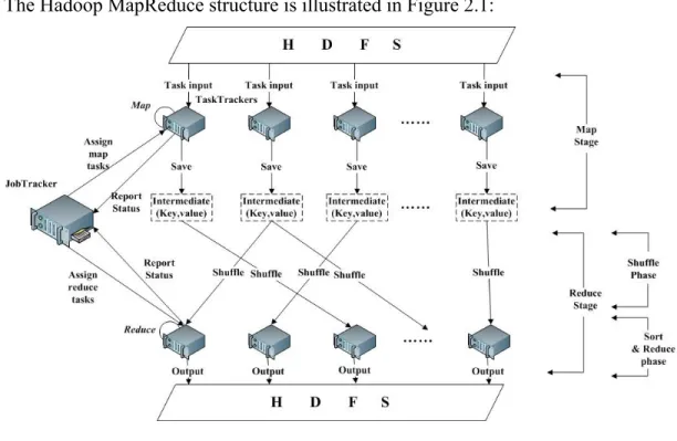
The Hadoop MapReduce structure is illustrated in Figure 2.1:

!

Figure 2.1 MapReduce Framework

as the master node and others as slave nodes. A Hadoop cluster uses Hadoop Distributed File System (HDFS) to manage its data. It divides each file into small fixed-size (e.g., 64 MB) blocks and stores several (e.g., 3) copies of each block in local disks of cluster ma-chines. A MapReduce computation is comprised of two stages, map and reduce, which take a set of input key/value pairs and produce a set of output key/value pairs. When a MapReduce job is submitted to the cluster, it is divided into M map tasks and R reduce tasks, where each map task will process one block (e.g., 64 MB) of input data.

A Hadoop cluster uses slave nodes to execute map and reduce tasks. There are limita-tions on the number of map and reduce tasks that a slave node can accept and execute simultaneously. That is, each slave node has a fixed number of map and reduce slots. Pe-riodically, a slave node sends a heartbeat signal to the master node. Upon receiving a heartbeat from a slave node that has empty map/reduce slots, the master node invokes the MapReduce scheduler to assign tasks to the slave node. A slave node that is assigned a map task reads the content of the corresponding input data block, parses input key/value pairs out of the block, and passes each pair to the user-defined map function. The map function generates intermediate key/value pairs, which are buffered in memory, and peri-odically written to the local disk and partitioned into R regions by the partitioning func-tion. The locations of these intermediate data are passed back to the master node, which is responsible for forwarding these locations to reduce tasks. A reduce task uses remote pro-cedure calls to read the intermediate data generated by the M map tasks of the job. Each reduce task is responsible for a region (partition) of intermediate data. Thus, it has to

re-trieve its partition of data from all slave nodes that have executed the M map tasks. This process is called shuffle, which involves many-to-many communications among slave nodes. The reduce task then reads in the intermediate data and invokes the reduce func-tion to produce the final output data (i.e., output key/value pairs) for its reduce partifunc-tion [2].

2.1.1 Task Scheduling & Data Locality

MapReduce framework has a very important feature that is different from traditional distributed computing environments like MPI, OpenMP, and computing Grid, etc. Tradi-tional frameworks move data to where the computation is while MapReduce moves com-putation to where data is. This way, MapReduce framework gets performance improve-ment through reduced network traffic. Thus, how to schedule MapReduce jobs becomes an important issue. In the following paragraphs, we will introduce MapReduce sched-uling mechanism and its data locality policy.

Hadoop MapReduce framework has a default FIFO scheduler. It schedules MapReduce jobs following a strict FIFO order, i.e., the second job will not be considered if the first job still has a task to be scheduled. Facebook [9] and Yahoo! [36] have developed multi-user schedulers in their production clusters, which will be described in the related work chapter. In the next two paragraphs, we introduce how the FIFO scheduler works and its data locality policy.

Hadoop default FIFO scheduler's data locality policy works as follows. First of all, when a slave node with empty map slots sends the heartbeat signal, the scheduler checks

the first job in the queue. If the job has map tasks whose input data blocks are stored in the slave node, the scheduler assigns the node one of these local tasks. If a slave node has more unused map slots, the scheduler will keep assigning local tasks to the node. Howev-er, if the scheduler can no longer find a local task from the first job, it assigns the node one and only one non-local task during this heartbeat interval, no matter how many free slots the node has.

For reduce stage, to evenly distribute reduce tasks to slave nodes, FIFO scheduler only assigns one reduce task to a node in a heartbeat interval because a worker node may be congested if it is assigned many reduce tasks of a job.

2.1.2 Speculative Execution

Since a parallel job's turnaround time is decided by its slowest task, to avoid a MapRe-duce job from being delayed by the slowest task, MapReMapRe-duce framework has a specula-tive execution policy that detects slow tasks and runs a duplicated copy of those tasks.

The MapReduce framework maintains task counters for every job. If a task is 1/3 slower than the average of a job's tasks' execution, the framework will launch another copy of this task on a different slave node. The faster of these two executions will be tak-en and the other one will be killed. This way, Hadoop MapReduce framework detects the straggler in advance to avoid further delay of execution. There are some researches for speculative execution including LATE [40], SAMR [41], and ESAMR [42], which will be introduced in the related work chapter.

2.1.3 Fault Tolerance

Fault tolerance is an important feature of Hadoop MapReduce. MapReduce clusters do not require sophisticated high-end servers to be used as worker nodes. This assumes that failures exist by default and happen frequently.

Failures are caused by many reasons, for example, network outage, hardware failure, users’ misconfiguration, and so on. MapReduce deals with failures through re-execution. Furthermore, Hadoop MapReduce framework has configurable timeout parameters to de-tect tasks without response. However, some failures cannot be resolved through re-execu-tion. Thus, the maximum-retry-times parameter is used to limit the maximum number of re-executions of a failed task.

For failures caused by an individual slave node, Hadoop MapReduce framework can blacklist a slave node that always fails to execute tasks. In this scenario, the system ad-ministrator needs to get involved to restore the blacklisted nodes.

2.1.4 YARN

Since previous Hadoop MapReduce clusters can only schedule MapReduce jobs, the system is not well utilized if users want to run other applications when the MapReduce cluster is not busy. Scientists and system architects proposed the next generation MapRe-duce framework (YARN) to resolve this problem. In the following paragraphs, we will explain YARN architecture.

!

Figure 2.2 YARN Architecture[2]

The basic idea of YARN is to split up the two major functionalities of the JobTracker, resource management and job scheduling/monitoring, into separate components. The idea is to have a global ResourceManager (RM), per-node NodeManager (NM), and per-ap-plication Apper-ap-plicationMaster (AM). In YARN, an apper-ap-plication is either a single job in the classical sense of a MapReduce job or a job described as a DAG (Directed Acyclic Graph, where a vertex is a processing stage and an edge represents data movement). Users are allowed to submit different types of jobs, create different kinds of AMs, and ask RM for resource allocation.

RM is responsible for allocating resources to the various running applications subject to constraints like capacities, priorities, etc. Here, the cluster resources are regarded as a

collection of LXCs (Linux containers) [43]. The "Slot" which is used in an older version of Hadoop MapReduce is not used anymore. The RM's scheduler does not monitor or track application status. Also, it offers no guarantees about restarting failed applications either due to application failure or hardware failures. This scheduler performs its sched-uling function based on the resource requirements of that application; which are ex-pressed in terms of resource containers that incorporate elements such as memory, CPU, disk, and network demands. The RM's scheduler has a policy plug-in, which is responsi-ble for partitioning the cluster resources among the various queues, applications etc. The current MapReduce schedulers such as the Capacity Scheduler [44] and the Fair Sched-uler [45] would be some examples of the plug-in. The RM and per-node slave, the NodeManager (NM), form the data-computation framework. The RM is the ultimate au-thority that arbitrates resources among all the applications in the system. The NM is the per-machine framework agent who is responsible for containers, monitoring their re-source usage (CPU, memory, disk, network), and reporting to the RM's scheduler. The per-application AM is, in effect, a framework specific library and is tasked with negotiat-ing resources from the RM and worknegotiat-ing with the NM(s) to execute and monitor the tasks. It is responsible for accepting job-submissions, negotiating the first container for execut-ing the application specific AM and provides the service for restartexecut-ing the AM container upon a failure. It also has the responsibility of negotiating appropriate resource containers from the RM scheduler.

re-sources including accelerators such as GPU [47], etc. AM can specify a set of NMs to run its tasks. For example, with label scheduling, an application that requires GPU can run on NMs that have GPU installed.

2.2 Hadoop Distributed File System

Hadoop Distributed File System (HDFS) is an essential component of the Hadoop framework.

HDFS is designed as a highly fault-tolerant, high throughput, and high capacity dis-tributed file system. It is ideal for storing terabytes or even petabytes of data on clusters that may be comprised of commodity hardware. HDFS is based on write-once-read-many and streaming access models. HDFS is very efficient in distributing and storing large amount of data.

2.2.1 HDFS Architecture

HDFS follows the master/slave architecture. The master node in the HDFS cluster is called the Namenode that manages the file system namespace and regulates client access-es to filaccess-es. There are a number of slave nodaccess-es, called Datanodaccess-es, which store actual data in units of blocks.

The Namenode maintains a mapping table that maps data blocks to Datanodes in order to process write and read requests from HDFS clients. It is also in charge of file system namespace operations like closing, renaming, and opening files and directories.

like replace, create, delete, and replicate from the Namenode. Figure 2.3 (adopted from Apache Hadoop Project) illustrates the HDFS architecture.

!

Figure 2.3 HDFS Architecture [2]

A Datanode periodically reports its status (including aliveness, data blocks, etc.) to the Namenode through sending messages (also called heartbeats) and asks the Namenode for instructions. The heartbeat can also help the Namenode to detect connectivity with its Datanodes. Every Datanode maintains an open server socket for data transferring from other Datanodes and user client(s). In order to keep the content of a Namenode in case of failures, HDFS allows a secondary Namenode to periodically backup Namenode data.

2.2.2 Data Placement and Fault-tolerance

of failure in a large-scale cluster becomes non-negligible. This means HDFS has to han-dle the scenario in which some components are non-functional.

HDFS employs an intelligent replica placement policy to guarantee reliability and per-formance. HDFS keeps 3 replicas for each data block by default. Once a data block is created, the first replica will be placed in a random node. The second replica will be placed in a node that is located in the same rack of that first node. The last replica will be stored in a node from a different rack to guarantee data availability even in the event that an entire rack is down.

2.2.3 Data Balancer

HDFS provides a balancer to equilibrate the disk usage among Datanodes. When plac-ing data blocks, the Namenode randomly picks a node to place the first copy of a data block. This mechanism may result in some nodes with smaller capacity having higher percentage of disk usage. The balancer is designed to solve this problem. It allows an administrator to balance HDFS Datanodes based on disk usage percentage.

2.4 GPGPU and CUDA

“General-Purpose Graphics Processing Unit (GPGPU) is utilizing the graphics-pro-cessing unit (GPU) to do computation for applications that are traditionally handled by the CPU” [33]. It is widely used in supercomputers as an accelerator to enhance the com-putational power. The comparison between CPU and GPU is detailed documented [33, 37-39].

CUDA [37] (Compute Unified Device Architecture) is a parallel computing architec-ture designed for GPUs and proposed by NVIDIA in 2006. It enables programmers to write C (C-CUDA) code to utilize GPUs for processing non-graphical data. C-CUDA programs are compiled using a specialized Path Scale Open64 C compiler. CUDA has been widely used to accelerate computations which otherwise take much longer or are intractable with the current technology, e.g., molecular dynamics simulation, electronic design automation, accelerated rendering of 3D graphics, speech indexing, and physical simulations.

With a design principle different from traditional CPUs, GPUs are based on a parallel throughput architecture that is aimed at executing a large number of concurrent threads slowly, as opposed to executing a single thread very fast. CUDA provides APIs for multi-ple operating systems, including Windows, Linux, and recently Mac OS X. Moreover, CUDA is supported by all GPUs recently designed and manufactured by NVIDIA [48], i.e., from the G8X series onwards, including GeForce, Quadro and the Tesla product lines. NVIDIA maintains compatibility among different generations of their GPUs such that CUDA programs developed for the GeForce 8 series will also work without modifi-cation on all future NVIDIA graphics cards.

With a radically different design, CUDA is superior over traditional GPGPU solutions with graphics APIs. For example, CUDA supports Scattered Reads, i.e., programs can access memory at arbitrary addresses on both the host and the device. Moreover, CUDA has a solid hardware implementation of floating-point arithmetic, which is essential for

scientific computations.

Admittedly, CUDA also suffers several drawbacks at the current stage. For instance, C-CUDA disallows the uses of recursion and function pointers, which might place a burden on programmers while developing CUDA programs in some scenarios. Although equipped with very fast internal cache memories, GPU might suffer from the limited bus bandwidth along the data-path to the CPU. Furthermore, the deep memory hierarchy and intricate internal mechanisms might have huge performance implications if CUDA pro-grams are written without accounting for such complexities in the design. Nevertheless, we believe the advantages of massive-parallelization offered by CUDA surely outweigh the drawbacks, as mentioned above, in real world applications.

Besides C, CUDA has bindings for most mainstream programming languages, includ-ing C++, Java, .NET, Perl, Python, Ruby, Lua, FORTRAN, and Matlab. In this work, we focus on JCuda [48], which is the CUDA binding for the Java language, which is being actively developed with support for the most recent CUDA API. JCuda provides a solid foundation for using CUDA libraries in Java applications.

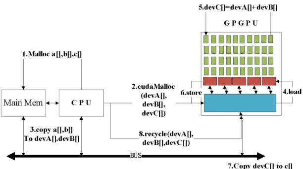
We use a very simple array summation example in Figure 2.4 to demonstrate how GPU and CPU cooperate together. In order to distinguish arrays in main memory from those in GPU’s global memory, we use “dev” (short for device) plus capital characters to identify three arrays in GPU’s global memory. First of all, CPU allocates three arrays in the main memory, array “a” and “b” contains elements we want to sum where array “c” is used to store the results (step 1). Correspondingly, CPU also needs to allocate three arrays

in GPU’s global memory that is the bottom rectangle in GPU (step 2). CPU copies array “a” and “b” contents from main memory into GPU’s global memory (step 3). On the GPU side, the first 4 rows of rectangles from top are computation elements and the fifth row of rectangles are shared memories. Communication between shared memories should employ global memory. The computation element needs to load array “devA” and “devB” into shared memories before launching the summation (step 4).

After the summation operation (step 5), array “devC” will be stored to global memory from shared memory (step 6). The next step is to copy array “devC” to array “c” from global memory to main memory (step 7). Finally, all memory space in shared memories and global memory will be recycled (step 8).

!

Figure 2.4 CPU + GPU Architecture

research reports: "On the Top500 Supercomputers list — a biannual ranking of super-computing sites around the world — the number of GPU-powered systems is rapidly growing. Today, three of the five fastest supercomputers in the world are NVIDIA GPU-powered. And these systems are much more energy efficient." More and more Hadoop clusters are equipped with GPUs to accelerate computational intensive MapReduce ap-plications [20-33]. In this dissertation, we will develop an energy efficient scheduler for Hadoop MapReduce clusters that have GPUs.

CHAPTER 3. RELATED WORK

MapReduce framework was first proposed by Google [1]. It is a fault-tolerant platform used for parallel processing huge amounts of data. Hadoop is a well-accepted open source implementation of Google’s MapReduce framework. In this dissertation, we focus on re-search work related to Hadoop MapReduce [2] from two aspects: scheduling and power management.

3.1 MapReduce Scheduling

Early versions of Hadoop had a very simple approach to scheduling users’ jobs: they ran in order of submission, using a FIFO scheduler by default. Typically, each job would use the whole cluster, so jobs had to wait their turn. As MapReduce clusters got popular, their scheduling became increasingly important. However, the default FIFO scheduler does not support many desired features like QoS guarantee, resource sharing, preemption, etc. Then, scientists started to explore various algorithms to improve MapReduce sched-uling [15-62]. In this section, we mainly focus on introducing research work from follow-ing areas that are related to my dissertation: detectfollow-ing speculative tasks, improvfollow-ing data locality, providing QoS guarantee, and scheduling MapReduce jobs in hybrid (CPU-GPU) clusters.

Hadoop’s scheduler implicitly assumes that cluster nodes are homogeneous and Map-Reduce tasks make progress linearly and uses these assumptions to decide when to specu-latively re-execute tasks that appear to be stragglers [2]. To overcome this limitation and

make the speculative execution mechanism effective in heterogeneous environments, re-searchers then developed LATE (Longest Approximate Time to End) scheduler [40], SAMR (Self-Adaptive MapReduce Scheduling) algorithm [41], and ESAMR algorithm [42].

MapReduce framework has a significant difference from previous parallel processing platforms, like computing Grid [63]. Previous frameworks move data to where the com-putation resource is located. However, MapReduce allocates the comcom-putation to where the data is stored. That is, when scheduling a task, MapReduce system will first consider a server that stores this task’s input data in local disk. To enhance this data locality in ex-ecuting MapReduce application, researchers have used technologies like prefetching [80], node status prediction [81], and delay scheduling algorithm [40].

In order to improve MapReduce cluster utilization, researchers introduce resource sharing [64-66], iterative execution [67-70], load balancing [72], online aggregation [73], genetic algorithm based data-aware group scheduling [74], introducing erasure cod-ing in storage [75], network-aware task placement schedulcod-ing [76], and multi-object scheduling [77] into MapReduce. Yahoo! developed a multi-queue scheduler called Ca-pacity Scheduler [44] for Hadoop clusters, where every queue is guaranteed a fraction of the capacity. Within a queue, it supports job priorities but no job preemption is allowed. To prevent one or more users from occupying all resources of a queue, each queue en-forces a limit on the percentage of resources allocated to a user at any given time if there is competition for resources.

The fair scheduler [40] also supports multiple queues (also called pools). Jobs are or-ganized into pools and resources are fairly divided between these pools. By default, there is a separate pool for each user so that each user gets an equal share of the cluster. Within each pool, jobs can be scheduled using either fair sharing or FIFO scheduling. Fair shar-ing schedulshar-ing is a method of assignshar-ing resources to jobs such that all jobs get, on aver-age, an equal share of resources over time. When there is a single job running, that job uses the entire cluster. When other jobs are submitted, task slots that free up are assigned to the new jobs so that each job gets roughly the same amount of CPU time. Unlike the default Hadoop FIFO scheduler, which forms a queue of jobs based on job arrival times, fair sharing scheduling mechanism guarantees that short jobs finish in reasonable time without starving long jobs. It provides an easy way to share a cluster between multiple users [40].

Since many MapReduce applications [73], including online data analytics for spam detection and ad optimization, require real-time data processing, scheduling real-time ap-plications in MapReduce Environment become an important problem[33,68-73]. Scien-tists have already established many important theories for real-time scheduling [90-98], especially in distributed systems [99-115]. For MapReduce real-time scheduling, J. Polo et al. [68] developed a scheduler that focuses on MapReduce jobs that have soft dead-lines. It estimates jobs’ execution times and tries to let jobs satisfy their deadlines by scheduling resources according to the estimated finishing times. Dong et al. [70] extend-ed the work by Polo et al., where a two-level MapRextend-educe schextend-eduler was developextend-ed to

schedule mixed soft real-time and non-real-time jobs according to their respective per-formance demands. Linh T.X. Phan et al [72] built HadoopRT that focuses on enhance-ment of EDF with locality-awareness and overload handling in cloud environenhance-ment. They defined a parameter to describe the execution time difference between local and non-local tasks. HadoopRT can adjust its scheduling policies according to this parameter to im-prove MapReduce applications' performance. Chen F. et al. proposed a system that schedule real-time MapReduce applications based on job size [115]. However, they did not consider energy consumption and hybrid clusters.

Kamal Kc et al. [69] developed a scheduler for MapReduce applications with hard deadlines. It also estimates the job finishing time according to available resources in a MapReduce cluster. If a job cannot finish before the hard deadline, the scheduler will not execute the job and will instead inform the user to adjust the job deadline. However, it has deficiencies that may cause deadline misses and low hardware utilization.

After YARN was created, scientists and architects started to improve its performance by optimizing the scheduling algorithms. Yao et al. [119] proposed YARN scheduler, named HaSTE, which can effectively reduce the make-span of MapReduce jobs in YARN by leveraging the information of requested resources, resource capacities, and dependen-cy between tasks. Lin et al. [120] employed real time ABS-YARN, which is a formal lan-guage for executable modeling of deployed virtualized software, to optimize the deploy-ment decision in the cloud to reduce scheduling cost.

emerged as major players in high performance computing [119-133]. For some types of MapReduce applications that require significant amount of computation (like machine learning and data mining algorithms), hybrid CPU-GPU architecture can be a high- per-formance, scalable, cost-effective, and power-efficient solution. [133-142].

B. Catanzaro et al. [135] created a platform that can automatically generate GPU CUDA code for MapReduce applications. J.A. Stuart et al. [20] also created a MapRe-duce framework on a cluster of GPUs to do volume rendering. Chen et al. [140] opti-mized MapReduce performance for GPU through reduction-based method that allows MapReduce to carry out reductions in shared memory. They designed and implemented their MapReduce framework in a single AMD Fusion chip. Qiao Z. et al. [138] built MR-Graph, an implementation of MapReduce, on a cluster of GPUs. F. Ji et al. [139] devel-oped and optimized performance for another MapReduce framework on GPU by consid-ering GPU multi-level memory hierarchy. However, all aforementioned frameworks did not focus on Hadoop MapReduce that is a widely accepted MapReduce platform. Liu LF. Et al. [142] developed an adaptive MapReduce framework for GPUs

K. Shirahata et al. [22] proposed a scheduling technique in hybrid CPU-GPU Hadoop MapReduce clusters, which minimizes job execution time via dynamic profiling of Map tasks running on CPU cores and GPU devices. However, they focused on optimizing the map stage of MapReduce applications and did not consider the energy consumption in their scheduling algorithm.

3.2 Power Management in Hadoop Cluster

With the increasing scale of MapReduce clusters, the cost of maintaining a MapReduce cluster becomes larger and larger. How to reduce MapReduce cluster power bill turns out to be a critical concern. Scientists have done some research work on power management of MapReduce clusters [144-148] inspired by previous theories in cluster power man-agement.

Lang et al. [143] provided an algorithm that only keeps the smallest number of servers that can guarantee data integrity in HDFS. However, it is not flexible if the cluster exe-cutes time-sensitive online applications. T. Wirtz et al. [144] used an experimental ap-proach to study the scalability of performance, energy, and efficiency of MapReduce for computation intensive workloads. They proposed a power management policy through resource allocation that changes the number of available workers and DVFS (Dynamic Voltage and Frequency Scaling) that adjusts the processor frequency based on current computational needs. M. Cardosa et al. [145] considered power management in cloud en-vironment through VMs management algorithm. Jerry Chou et al. [146] built an algo-rithm that can monitor system utilization and re-direct requests to existing powered-on recourses. N. Yigitbasi et al. [147] investigated scheduling algorithm in a heterogeneous cluster made of high performance nodes and low power nodes. His scheduling algorithm is limited in this specific hardware environment. Chen et al. [148] presented BEEMR through tracing MapReduce interactive analytics in Facebook Hadoop production cluster. It first categorizes MapReduce applications into different job zones according to service

types, for example, batching jobs, interactive jobs, etc. Then, BEEMR saves energy by flexibly adjusting the number of servers that work for interactive jobs according to sys-tem requests. However, it is based on Facebook’s workload that is mainly composed of online queries. It may not be a good fit for MapReduce clusters that work in other indus-tries like banks, health care companies, etc.

Since hybrid CPU-GPU cluster becomes more and more popular, scientists start to consider how to predict hybrid CPU-GPU cluster power consumption. Ren DQ et al. [149] proposed an empirical power model for GPU to predict the optimal number of ac-tive processors (CPU and GPU) for a given application. W. Liu et al. created a waterfall model [150] which uses a mapping algorithm to apply different energy saving strategies to keep the system at lower energy levels. In their mapping algorithm, they adopted dy-namic voltage scaling, dydy-namic resource scaling and -migration for GPU to reduce ener-gy consumption. H. Huo et al. [151] proposed a flexible enerener-gy efficient task-scheduling scheme for heterogeneous tasks in the heterogeneous GPU-enhanced clusters. It includes a system model to describe hardware heterogeneity and a task model to characterize ap-plication heterogeneity in a cluster. However, they provide no evaluation data from either simulation or real-system experiment. Kim et al. [153] proposed an algorithm about pow-er management in MapReduce hybrid clustpow-er. But they did not considpow-er data locality.

In summary, the previous research works outlined here do not consider multiple con-straints including energy efficiency, data locality, and throughput together in the hybrid heterogeneous Hadoop clusters. Instead, this dissertation will focus on resolve this hard

CHAPTER 4. MATCHMAKING SCHEDULER

In a MapReduce cluster, data are distributed to individual nodes and stored in their disks. To execute a map task on a node, we need to first have its input data available on that node. Since transferring data from one node to another takes time, delays task execu-tion, and consumes extra energy. An efficient MapReduce scheduler must avoid unneces-sary data transmission.

We will focus on the problem of decreasing data transmission in a MapReduce cluster and we develop a scheduling technique to improve map tasks’ data locality rate. For a given execution of MapReduce workload, the data locality ratial is defined in this disser-tation as the ratio between the numbers of local map tasks and all map tasks, where a lo-cal map task refers to a task that has been executed on a node that contains its input data. A low data locality rate means more data transfer between machines and higher network traffic. To avoid unnecessary data transfer, our scheduling technique aims to achieve high data locality rate and also short response time for MapReduce clusters. We developed a new technique to enhance the data locality. The main idea of the technique is as follows. To assign tasks to a node, local map tasks are always preferred over non-local map tasks, no matter which job a task belongs to, and a locality marker is used to mark nodes and to ensure each node a fair chance to grab its local tasks. Experiments are carried out to eval-uate the aforementioned techniques and experimental results show that our technique leads to the high data locality rate and the low response time for map tasks. Unlike the delay algorithm [40], our technique does not require the tuning of the delay parameter.

4.1 Hadoop Default FIFO Scheduler

The Hadoop default FIFO scheduler has already taken data locality into account. When a slave node with empty map slots sends the heartbeat signal, the MapReduce scheduler checks the first job in the queue. If the job has map tasks whose input data blocks are stored in the slave node, the scheduler assigns the node one of these local tasks. If a slave node has more unused map slots, the scheduler will keep assigning local tasks to the node. However, if the scheduler can no longer find a local task from the first job, it as-signs the node one and only one non-local task during this heartbeat interval, no matter how many free slots the node has.

This default FIFO scheduler, however, has deficiencies. First of all, it follows the strict FIFO job order to assign tasks, which means it will not allocate any task from other jobs if the first job in the queue still has an unassigned map task. This scheduling rule has a negative effect on the data locality because another job’s local tasks cannot be assigned to the slave node unless the first job has all its map tasks (many of which are non-local to the node) scheduled.

Secondly, the data locality is randomly decided by the heartbeat sequence of slave nodes. If we have a large cluster that executes many small jobs, the data locality rate could be quite low. As mentioned, in a MapReduce cluster, tasks are assigned to a slave node in response to the node’s heartbeat. With the FIFO scheduler, heartbeats are also processed in a FIFO order and a node is assigned a non-local map task when there is no local task from the first job. In a large cluster many nodes heartbeat simultaneously.

However, a small job has less input data that are stored in a small number of nodes. It is thus a high probability event that the scheduler assigns tasks to slave nodes that do not have the small job’s input data but give heartbeats first. For example, if we execute a job of 5 map tasks on a MapReduce cluster of 100 slave nodes, it is unlikely to get a high lo-cality rate. Since each map task needs one input data block, which by default has 3 repli-cas stored in 3 nodes, at most 15 out of 100 nodes have input data for the job, i.e., the job’s tasks are all non-local to at least 85 nodes. A slave node with empty map slots that sends in a heartbeat first will always be assigned at least one map task, local or non-local. It is highly likely that the job’s tasks will be assigned to many of those 85 nodes which do not have the input data blocks before a node even gets a chance to grab a local task from the job.

4.2 Delay Scheduling Algorithm

Zaharia et al. [40] have developed a delay scheduling algorithm to improve the data locality rate of Hadoop clusters. It relaxes the strict job order for task assignment and de-lays a job’s execution if the job has no map task local to the current slave node. To assign tasks to a slave node, the delay algorithm starts the search at the first job in the queue for a local task. If not successful, the scheduler delays the job’s execution and searches for a local task from succeeding jobs. A maximum delay time D is set. If a job has been

skipped long enough, i.e., longer than D time units, its non-local tasks will then be

as-signed for execution. With the delay scheduling algorithm, a job’s execution is postponed to wait for a slave node that contains the job’s input data. Here, the delay time D is a key

parameter. By default, it is set at 1.5 times the slave node’s heartbeat interval. However, to obtain the best performance for the delay scheduling algorithm, we have to choose an appropriate D value. If the value is set too large, job starvations may occur and affect

per-formance. On the contrary, a too small D value allows non-local tasks to be assigned too

fast. For different kinds of workloads and hardware environments, the best delay time may vary. To get an optimal delay time always requires careful D value tuning.

In addition, this delay algorithm allows a node to obtain multiple non-local map tasks in a heartbeat interval if the node has more than one free slot. In some situations, this al-gorithm could perform worse than the FIFO scheduler’s locality enhancement policy be-cause the latter only allows one non-local task to be assigned to a node in a heartbeat in-terval.

Although first developed to improve the data locality of the Hadoop fair scheduler [20], delay scheduling is applicable beyond fair sharing, in general, applicable to any scheduling policy (e.g., FIFO) that defines an order in which jobs should be given re-sources [2]. It is very popular and widely used in Hadoop clusters.

4.3 Matchmaking Scheduling Algorithm

This section presents our new technique for enhancing the data locality in MapReduce clusters. The main idea behind our technique is to give every slave node a fair chance to grab local tasks before any non-local tasks are assigned to any slave node. Since our algo-rithm tries to find a match, i.e., a slave node that contains the input data, for every unas-signed map task, we call our new technique the matchmaking scheduling algorithm.

First of all, like the delay scheduling algorithm, our matchmaking algorithm also relax-es the strict job order for task assignment. If a local map task cannot be found in the first job, the scheduler will continue searching the succeeding jobs. Second, in order to give every slave node a fair chance to grab its local tasks, when a node fails to find a local task in the queue for the first time in a row, no non-local task will be assigned to the node. That is, the node gets no map task for this heartbeat interval. Since during a heartbeat in-terval, all slave nodes with free map slots have likely given their heartbeats and been con-sidered for local task assignment, when a node fails to find a local task for the second time in a row (i.e., still no local task a heartbeat interval later), to avoid wasting comput-ing resources, the matchmakcomput-ing algorithm will assign the node a non-local task. This way, our algorithm achieves not only high data locality rate but also high cluster utiliza-tion. To enforce the aforementioned rule, our algorithm gives every slave node a locality marker to mark its status. If none of the jobs in the queue has a map task local to a slave node, depending on this node’s marked value, the matchmaking algorithm will decide whether or not to assign the node a non-local task. Third, our matchmaking algorithm al-lows a slave node to take at most one non-local task every heartbeat interval. At last, all slave nodes’ locality markers will be cleared when a new job is added to the job queue. Because a new job may comprise new local tasks for some slave nodes, upon the new job’s arrival, our algorithm resets the status of all nodes and again starts the all-to-all task-to-node matchmaking process. Tables 4.1 and 4.2 give the pseudo code of our algo-rithm. Like delay scheduling algorithm, our matchmaking algorithm is applicable to any

scheduling policy (e.g., FIFO or fair sharing scheduling) that defines an order in which jobs should be given resources.

Table 4.1 Matchmaking Algorithm

Algorithm 1: Matchmaking Scheduling Algorithm 1: for each node i of the N slave nodes do 2: set LocalityMarker[i]=null

3: end for

4: //Upon receiving a heartbat from node i:

5: while node i has free slots, i.e., its free slot count s>0 6: set previousMarker=LocalityMarker[i]

7: for each job j in the JobQueuedo

8: if job j has an unassigned local task tthen 9: assignt to node i 10: set s=s-1 11: ifLocalityMarker[i]==nullthen 12: LocalityMarker[i]=1 13: elseLocalityMarker[i]+=1 14: end if 15: break for 16: else continue 17: end if 18: end for 19: ifpreviousMarker==LocalityMarker[i] then 20: setLocalityMarker[i]=0 //mark this node

21: break while

22: elseifLocalityMarker[i]==0then

23: assign node i a non-local task t’ from the first job in the JobQueue 24: set s=s-1

25: break while 26: end if

Table 4.2 Locality Marker Maintenance

4.4 Evaluation of Different Data Locality Policies

To evaluate our matchmaking scheduling algorithm, we compare it with the Hadoop default FIFO scheduler and the delay scheduling algorithm. Two metrics, i.e., map tasks’

data locality ratio and average response time, are used for evaluation.

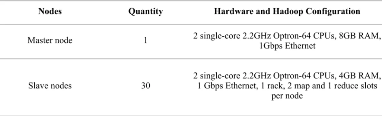
We run experiments in a private cluster of 1 head node and 30 slave nodes that are con-figured as one rack. We modify Hadoop and integrate our matchmaking algorithm with both Hadoop FIFO scheduler and Hadoop fair scheduler. The cluster is configured with a block size of 128MB, which follows Facebook’s Hadoop cluster block size configuration [20]. Table 4.3 lists our Hadoop cluster hardware environment and configuration.

Table 4.3 Experimental Environment

4.4.1 Experimental Environment

To evaluate our matchmaking algorithm, we create a submission schedule that is simi-Algorithm 2: Locality Marker Cleaning simi-Algorithm

1: //When a new job j is added into the JobQueue: 2: for each node i of the N slave nodes do 3: set LocalityMarker[i]=null

4: end for

Nodes Quantity Hardware and Hadoop Configuration

Master node 1 2 single-core 2.2GHz Optron-64 CPUs, 8GB RAM, _{1Gbps Ethernet}

Slave nodes 30 2 single-core 2.2GHz Optron-64 CPUs, 4GB RAM, 1 Gbps Ethernet, 1 rack, 2 map and 1 reduce slots per node

lar to the one used by Zaharia et al[20]. They generated a submission schedule for 100 jobs by sampling job inter-arrival times and input sizes from the distribution seen at Facebook over a week. By sampling job inter-arrival times at random from the Facebook trace, they found that the distribution of inter-arrival times was roughly exponential with a mean of 14 seconds.

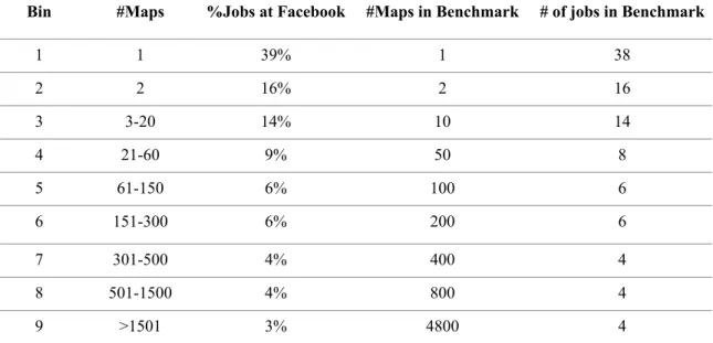
They also generated job input sizes based on the Facebook workload, by looking at the distribution of the number of map tasks per job at Facebook and creating datasets with the correct sizes (because there is one map task per 128 MB input block). Job sizes were quantized into nine bins, listed in Table 4.4 [20], to make it possible to compare jobs in the same bin within and across experiments. Our submission schedule has similar job sizes and job inter-arrival times. In particular, our job size distribution follows the first six bins of job sizes shown in Table 3.4, which cover about 89% of the jobs at the Facebook production cluster. Because most jobs at Facebook are small and our test cluster is limited in size, we exclude those jobs with more than 300 map tasks. Like the schedule in [20], the distribution of inter-arrival times is exponential with a mean of 14 seconds, making our submission schedule totally 21 minutes long.

We generate 100 input data blocks in Hadoop Distributed File System (HDFS). The popularity of blocks is assumed to follow a uniform distribution. That is, when a job re-quests a block, it is evenly likely to be any one of the blocks stored in HDFS. Each of the blocks has 2 replicas. We distribute and store these 200 block replicas evenly in 30 slave nodes, ensuring no two replicas of a block be stored in the same node. As a result, every

slave node contains about 6 (or 7) blocks. By uniformly distributing blocks among our cluster nodes, we avoid hotspots of data requests.

We use our submission schedule for two application workloads. One is loadgen that is

a test example from the Hadoop test package. It loads input data and outputs a fraction of the data intact. This application has been used as a test workload for the delay algorithm [20]. The other application we adopt is wordcount that is a classic example of Hadoop

applications.

As mentioned, we have modified Hadoop and integrated our matchmaking algorithm with both Hadoop FIFO scheduler and Hadoop fair scheduler.

In our experiments, we always configure the cluster to have just one job queue. With Hadoop fair scheduler, all jobs in a queue are scheduled following either fair sharing or FIFO scheduling rule. With fair sharing scheduling, resources are assigned to jobs such that all jobs get, on average, an equal share of resources over time. We have tested the performance of delay algorithm within Hadoop fair scheduler. Depending on the applied scheduling rules (FIFO or fair sharing), we have two different versions: FIFO with delay algorithm and Fair with delay algorithm. Since we have tested our matchmaking algo-rithm within Hadoop FIFO scheduler, when testing matchmaking algoalgo-rithm within Hadoop fair scheduler, only the fair sharing scheduling rule is applied.

We thus run each workload under five schedulers: Hadoop FIFO scheduler, Hadoop FIFO scheduler with matchmaking algorithm, FIFO with delay algorithm, Fair with delay algorithm, and Fair with matchmaking algorithm.

For the delay algorithm, we need to configure the maximum delay time D. In our

ex-periments, a total of 8 different D values are chosen. They are from 0.1 to 10 times the

slave node’s heartbeat interval. Since we configure the heartbeat interval to be 3 seconds long, the maximum delay time D changes from 0.3 to 30 seconds.

To eliminate the possible randomness of cluster hardware status, every point shown in the figures is the average of three runs.

Table 4.4 Facebook Workload

4.4.2 Experiments

We first use the data locality rate to measure the performance of the following three schedulers: Hadoop FIFO scheduler, Hadoop FIFO scheduler with matchmaking algo-rithm, and FIFO with delay algorithm. Given a workload execution, the data locality rate is defined as,

Bin #Maps %Jobs at Facebook #Maps in Benchmark # of jobs in Benchmark

1 1 39% 1 38 2 2 16% 2 16 3 3-20 14% 10 14 4 21-60 9% 50 8 5 61-150 6% 100 6 6 151-300 6% 200 6 7 301-500 4% 400 4 8 501-1500 4% 800 4 9 >1501 3% 4800 4

Data Locality Rate=! (4.1)

where l is the number of local map tasks and n is the total number of map tasks. To

make the figures properly fits the page, we did not follow numerical scale of delay times in x coordinate but simply listed them side by side to show the trend of data locality rate when delay time increases.

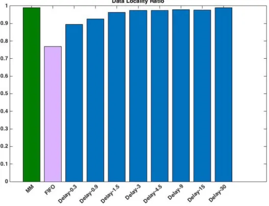
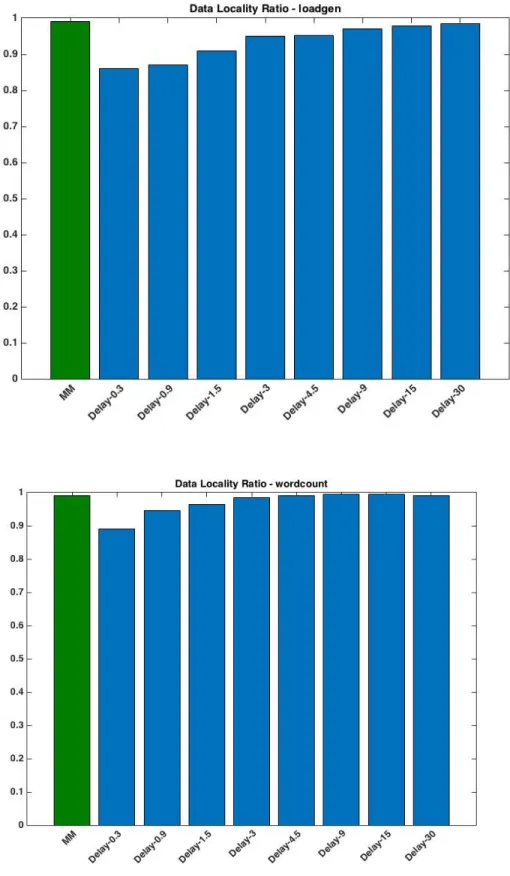
Our experimental results on data locality rate with the two application workloads are shown in Figures 4.1 and 4.2. As we can see, the data locality rate achieved with the de-lay algorithm increases with the maximum dede-lay time D. The longer a job is delayed, the

higher the probability that the job finds slave nodes that contains the input data blocks. In following diagrams, we use MM to represent Matchmaking algorithm.

Figure 4.1 Loadgen Workload: Data Locality Ratio

!

!

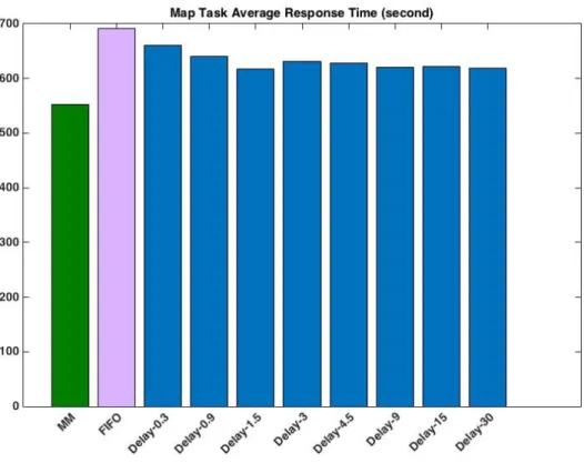
Figure 4.3 Loadgen Workload: Map Tasks' Average Response Time

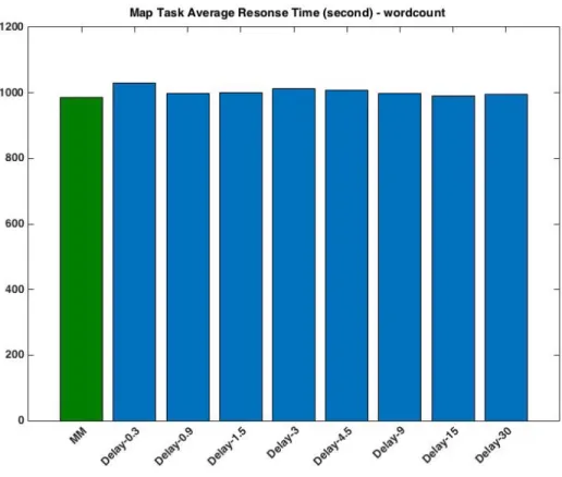
Figure 4.4 Wordcount Workload: MapTasks' Average Response Time

Figures 4.1 and 4.2 also show that the FIFO scheduler leads to the worst performance, i.e., the lowest data locality rate. However, when we integrate our matchmaking tech-nique with the FIFO scheduler, the algorithm achieves the highest data locality rate, bet-ter than any of those achieved with the delay algorithm of different D values.

To evaluate the algorithms’ performance only via the data locality rate is not enough since we can easily design an algorithm that enforces the constraint that all tasks have to be executed on slave nodes that contain their input data, leading to 100% data locality rate but also long response time for map tasks due to the long delay required to satisfy the strict constraint. Therefore, we also evaluate our algorithms by another metric: the aver-age response time of all map tasks. Figures 4.3 and 4.4 present the experimental results. As shown in the figures, when we run the workloads with the FIFO scheduler, we get the longest average response time for map tasks. After enhancing the FIFO scheduler with our matchmaking algorithm, we reduce the average response time significantly.

For the delay algorithm, although the higher the D value, the better the data locality rate (see Figures 4.1 and 4.2), the relationship between the D value and the average re-sponse time is not so straightforward. When running the loadgen workload, the average response time varies with the D value, e.g., getting smaller when D increases from 0.3 to 1.5 seconds but longer when D increases from 1.5 to 3 seconds (see Figure 4.3). The low-est average response time is achieved when the maximum delay time is set at 30 seconds (see Figures 4.1 & 4.3-loadgen). But, that is not the optimal D value when running the

wordcount workload. As shown in Figure 4.2 (and also in Figure 4.4-wordcount), when D = 9 or 15 seconds, we get the best average response time for the wordcount workload. In neither cases, the default configuration (i.e., D = 4.5 seconds, 1.5 times the heartbeat in-terval) leads to the best performance. This group of experiments demonstrates that for different workloads, the best delay parameter varies, indicating the necessity of parameter tuning for the delay algorithm. However, our matchmaking algorithm does not require this intricate parameter tuning process. For both workloads, the FIFO scheduler with our matchmaking algorithm achieves the lowest average response time, better than that achieved by the optimally configured delay algorithm.

Let tavg represent the average response time of all map tasks. It equals to the summa-tion of two parts. That is,

! (4.2)

where Rl denotes the data locality rate, ! ! represents the average response time of all local map tasks, and ! the average response time of all non-local map tasks.

Because network bandwidth is a relatively scarce resource in a MapReduce cluster [1,2] and the network data transferring rate is slower than the disk access rate when MapReduce was first developed, a local map task’s execution is often much faster than that of a non-local map task. Therefore, according to Equation (4.2), increasing the data locality rate Rl tends to decrease the average response time of all map tasks tavg. On the other hand, with the delay algorithm, as the maximum delay time D increases, a job and

its tasks’ execution is allowed to be delayed for a longer time. As a result, although Rl increases, both ! and ! increase as well, leading to the potential increase of tavg. This explains why map tasks’ average response time does not decrease monotonically with the increase of the maximum delay time D.

So far, we have used experiments to compare three schedulers: Hadoop FIFO sched-uler, Hadoop FIFO scheduler with matchmaking algorithm, and FIFO with delay algo-rithm. The results show that the FIFO scheduler with matchmaking algorithm achieves the highest locality rate and the lowest map task response time without the parameter tun-ing hassle. Next, to further compare the delay algorithm and our matchmaktun-ing algorithm, we integrate the matchmaking algorithm into Hadoop fair scheduler and compare the fol-lowing two schedulers: fair scheduler with delay algorithm and fair with matchmaking algorithm.

Figures 4.5 and 4.6 show the data locality rate and the map tasks’ average response time for the Hadoop fair schedulers.

We can see that when integrated with the fair sharing scheduling, our matchmaking algorithm still achieves better data locality rates and near-optimal average response times. More importantly, our algorithm achieves this great performance without the necessity of parameter tuning.

!

!

!

CHAPTER 5. REAL-TIME MAPREDUCE SCHEDULER

With the increasing popularity of MapReduce, more and more applications were de-veloped to employ this powerful platform. Some applications are sensitive to time. For example, financial companies require data to be processed in an acceptable time interval. A scheduler that supports real-time applications became more and more important.

In this section, we will introduce our Real-Time MapReduce (RTMR) scheduler to not only provide deadline supports for MapReduce applications executing in heterogeneous environments but also ensure good cluster utilization. The following of this section is or-ganized as follows; first, we briefly describe the Deadline Constraint scheduler [17] and its deficiencies. And then, our scheduling algorithm is presented in detail. Evaluations of these two schedulers are provided in the end.

5.1 Deadline Constraint Scheduler

The Deadline Constraint Scheduler [17] aims to ensure deadlines for real-time Map-Reduce jobs. After a job is submitted, the scheduler first determines whether the job can be completed within the specified deadline or not using a schedulability test:

It assumes that all reduce tasks of a job will start executing simultaneously for the same amount of time that is known a priori. Based on this assumption, the Deadline Con-straint Scheduler calculates the latest reduce start time for the job to meet its deadline. If sm is the map start time of the job, then the maximum time for the job to complete its map stage is. Unlike for the reduce stage, the Deadline Constraint Scheduler assumes that

each job executes at a minimum degree of task parallelism for the map stage. That is, the scheduler only assigns the job the minimum number of map slots that are required to meet its deadline. However, it demands all map slots to be available simultaneously at to run the job’s map tasks. Assume the job’s input data size is σ and the cost (i.e., time) of processing a unit data in a map task is seconds, then, the scheduler calculates as:

! . (5.1)

The Deadline Constraint scheduler, however, has some limitations and deficiencies, which may lead to resource underutilization and deadline violations. First, because the scheduler assumes that all reduce tasks of a job start to run simultaneously, it cannot ac-cept a job with more reduce tasks than the cluster’s total number of reduce slots. Second, by checking the aforementioned two conditions in the schedulability test, the scheduler only considers a single scenario where the job’s deadline might be satisfied. Those condi-tions are, however, unnecessary for meeting a job’s deadline. Many jobs that do not pass the test can nevertheless be accepted and completed by their deadlines. For instance, even if the system does not have number of map slots available upon the job’s arrival, the job can still finish its map stage on time and meet the job’s deadline if we have more re-sources available at a later time point. Furthermore, the constraint scheduler does not consider the case where slots become available and utilized at different time points. Due to these reasons, the Deadline Constraint scheduler rejects tasks unnecessarily and cannot well utilize system resources.