Author's personal copy

Thermoeconomic analysis of a novel zero-CO

2

-emission high-efficiency power

cycle using LNG coldness

Meng Liu

, Noam Lior

_{, Na Zhang}

_{, Wei Han}

China National Institute of Standardization, Beijing 100088, PR China

b

Institute of Engineering Thermophysics, Chinese Academy of Sciences, P.O. Box 2706, Beijing 100190, PR China

c

Department of Mechanical Engineering and Applied Mechanics, University of Pennsylvania, Philadelphia, PA 19104-6315, USA

a r t i c l e

i n f o

Article history:

Received 30 November 2008 Accepted 29 June 2009 Available online 12 August 2009 Keywords:

Oxy-fuel power system LNG Coldness energy Power generation Thermoeconomics CO2capture

a b s t r a c t

This paper presents a thermoeconomic analysis aimed at the optimization of a novel zero-CO2and other emissions and high-efficiency power and refrigeration cogeneration system, COOLCEP-S (Patent pend-ing), which uses the liquefied natural gas (LNG) coldness during its revaporization. It was predicted that at the turbine inlet temperature (TIT) of 900°C, the energy efficiency of the COOLCEP-S system reaches 59%. The thermoeconomic analysis determines the specific cost, the cost of electricity, the system pay-back period and the total net revenue. The optimization started by performing a thermodynamic sensi-tivity analysis, which has shown that for a fixedTITand pressure ratio, the pinch point temperature difference in the recuperator,DTp1, and that in the condenser,DTp2are the most significant uncon-strained variables to have a significant effect on the thermal performance of novel cycle. The payback per-iod of this novel cycle (with fixed net power output of 20 MW and plant life of 40 years) was5.9 years at most, and would be reduced to3.1 years at most when there is a market for the refrigeration byproduct. The capital investment cost of the economically optimized plant is estimated to be about 1000 $/kWe, and the cost of electricity is estimated to be 0.34–0.37 CNY/kWh (0.04 $/kWh). These values are much lower than those of conventional coal power plants being installed at this time in China, which, in con-trast to COOLCEP-S, do produce CO2emissions at that.

Ó2009 Elsevier Ltd. All rights reserved.

1. Introduction

Natural gas is one of the most widely used fossil energy re-source with higher heat value and less pollutant production than the other fossil energy resources. Since the first liquefied natural gas (LNG) trade in 1964, the global LNG trade has seen a continu-ously rapid growth, mainly because the transformation from natu-ral gas to the LNG reduces its volume by about 600-fold and thus facilitates the conveyance from the gas source to receiving termi-nal. Liquefaction of the gas to LNG requires, however, approxi-mately 500 kWh electric energy per ton LNG, It is noteworthy that the LNG, at about 110 K, thus contains a considerable portion of the energy and exergy that were invested in this process. The principle of the novel COOLCEP-S system is the effective use of that stored potential during the revaporization and heating to approxi-mately ambient temperature of the LNG for pipeline transmission to the consumers. This use of the valuable energy and exergy re-places the commonly employed revaporization methods of using ambient (ocean or air) or gas combustion heat, which simply waste it and may also cause undesirable environmental effects.

Recovery of the cryogenic exergy in the LNG evaporation pro-cess by incorporating this propro-cess into a properly designed ther-mal power cycle, in different ways, has been proposed in a number of past publications [1–13]. This includes methods which use the LNG as the working fluid in natural gas direct expansion cycles, or its coldness as the heat sink in closed-loop Rankine cycles [1–6], Brayton cycles [7–9], and combinations thereof[10,11]. Other methods use the LNG coldness to improve the performance of conventional thermal power cycles. For example, LNG vaporization can be integrated with gas turbine in-let air cooling [5,12] or steam turbine condenser system (by cooling the recycled water[11]), etc. Some pilot plants have been established in Japan from the 1970s, combining closed-loop Ran-kine cycles (with pure or mixture organic working fluids) and di-rect expansion cycles[1].

Increasing concern about greenhouse effects on climate change prompted a significant growth in research and practice of CO2

emission mitigation in recent years. The main technologies pro-posed for CO2capture in power plants are physical and chemical

absorption, cryogenic fractionation, and membrane separation. The amount of energy needed for the CO2capture would lead to

the reduction of power generation energy efficiency by up to 10 percentage points[14,15].

0196-8904/$ - see front matterÓ2009 Elsevier Ltd. All rights reserved. doi:10.1016/j.enconman.2009.06.033

* Corresponding author.

E-mail addresses:[email protected](M. Liu),[email protected](N. Lior).

Contents lists available atScienceDirect

Energy Conversion and Management

Beside the efforts for reduction of CO2emissions from existing

power plants, concepts of power plants having zero-CO2-emission

were proposed and studied. Oxy-fuel combustion is one of the pro-posed removal strategies. It is based on the close-to-stoichiometric combustion, where the fuel is burned with enriched oxygen (pro-duced in an air separation unit, ASU) and recycled flue gas. The combustion is accomplished in absence of the large amounts of nitrogen and produces only CO2and H2O. CO2separation is

accom-plished by condensing water from the flue gas and therefore re-quires only a modest amount of energy. Some of the oxy-fuel cycles with ASU and recycled CO2/H2O from the flue gas are the

Graz cycle, the Water Cycle, and the Matiant cycle[16–20]. We proposed and analyzed the semi-closed oxy-fuel cycles with inte-gration of the LNG cold exergy utilization[21,22]. The additional power use for O2production amounts to 7–10% of the cycle total

input energy. To reduce the oxygen production efficiency penalty, new technologies have been developed, such as chemical looping combustion (CLC)[23,24]and the AZEP concept[25], employing, respectively, oxygen transport particles and membranes to sepa-rate O2from air. Kvamsdal et al.[26]made a quantitative

compar-ison of various cycles with respect to plant efficiency and CO2

emissions, and concluded that the adoption of these new technol-ogies shows promising performance because no additional energy is then necessary for oxygen separation, but they are still under development.

We proposed and analyzed a novel zero-CO2-emission power

cycle using LNG coldness, with the name of COOLCEP-S[27], which is based on the concept proposed by Deng et al.[6]: that is a cogen-eration (power and refrigcogen-eration) recuperative Rankine cycle with CO2as the main working fluid. Combustion takes place with

natu-ral gas burning in an oxygen and recycled-CO2mixture. The high

turbine inlet temperature and turbine exhaust heat recuperation present a high heat addition temperature level, and the heat sink at a temperature lower than the ambient accomplished by heat ex-change with LNG offer high power generation efficiency. At the same time, these low temperatures allow condensation of the working fluid and the combustion-generated CO2is thus captured.

Furthermore, the sub-critical re-evaporation of the CO2 working

fluid is accomplished below ambient temperature and can thus provide refrigeration if needed.

The primary advances over the work presented in[6]are the integration of the LNG evaporation with the CO2 condensation

and capture. In the analysis in[6], it was assumed that LNG con-sists of pure CH4and the combustion production after water

re-moval can be fully condensed at the 5.3 bar/53.1°C. In COOLCEP-S, we used a different condensation process: first the amount of the working fluid needed for sustaining the process is condensed and recycled, and the remaining working fluid, having a relatively small mass flow rate (<5% of the total turbine exhaust flow rate after water removal) and higher concentration of noncon-densable gases, are compressed to a higher pressure level and then condensed. Alternatively, the CO2-enriched flue gas can be

con-densed at a lower temperature, which can be provided by the LNG coldness, but it would then freeze the CO2and is thus not

con-sidered in this paper; instead we adopted a higher condensation pressure for the flue stream condensation, which leads to a more conservative solution and some efficiency penalty but can recover the CO2fully. It is found that, at the turbine inlet temperature of

900°C and the pressure ratio of four, the energy efficiency of the COOLCEP-S cycle reaches 59%.

In this study we performed a thermoeconomic analysis of that system, to determine the conditions and costs for optimal system operation and configuration. A much more limited paper on the subject was presented as[28].

Consider the thermoeconomic analysis, the recuperator and the CO2condenser are the two most important heat exchangers in the

COOLCEP-S cycle in their effect on performance and cost. In this paper, we conduct a thermoeconomic optimization of the pinch point temperature differences, the DTp1 in the recuperator and

the DTp2in the CO2 condenser, based on the cycle thermal and

exergy efficiencies, and the economic performance evaluation cri-teria that include the plant specific cost, the cost of electricity, the payback period and the total net revenue, to find the thermo-economically optimal values ofDTp1andDTp2.

2. System configuration description

Fig. 1shows the layout of the COOLCEP-S cycle, which consists of a power subcycle and an LNG vaporization process.Fig. 2is the cyclet–sdiagram. The interfaces between the power subcycle and the LNG vaporization process are the CO2condenser CON, the heat

exchangers HEX1, and the fuel feed stream 8.

The power subcycle can be identified as 1-2-3-4-5-6-7-8-9-10-11-12/13-14-1. The low temperature (50°C) liquid CO2 as the

main working fluid (1) is pumped to about 30 bar (2), then goes through a heat addition process (23) in the evaporator EVA1 and can thereby produce refrigeration if needed. The O2(4)

pro-duced in an air separator unit (ASU) is compressed and mixed with the main CO2working fluid. The gas mixture (6) is heated (6–7) by

turbine (GT) exhaust heat recuperation in REP.The working fluid temperature is further elevated in the combustor B, fueled with natural gas (8), to its maximal value (the turbine inlet temperature

TIT) (9). The working fluid expands to the working fluid condensa-tion pressure (10) in the gas turbine (GT) to generate power and is then cooled (to 11) in the recuperator REP.

The gases in the mixture at the exit of REP (11) need to be sep-arated, and the combustion-generated CO2component needs to be

condensed for ultimate sequestration, and this is performed by fur-ther cooling: in the LNG-cooled heat exchanger HEX1, in which the H2O vapor in the mixture is condensed and drained out (12).

After-wards, the remaining working gas (13) is condensed (14) in the condenser CON against the LNG evaporation, and recycled (1). The remaining working fluid (15) enriched with noncondensable species (mainly N2, Ar and O2) is further compressed in C3 to a

higher pressure level under which the combustion-generated CO2

is condensed and captured, ready for final disposal.

The LNG vaporization process is 18-19-19a/b-20a/b-20-21-22-23/8. LNG (18) is pumped by P2 to the highest pressure (73.5 bar), typical for receiving terminals which supply long dis-tance pipeline network, and then evaporated with the heat addi-tion from the power cycle. The evaporated NG (natural gas) may produce a small amount of cooling in HEX3 if its temperature is still low enough at the exit of HEX1, and thus contribute to the overall system useful outputs. Finally, the emerging natural gas stream is split into two parts where most of it (23) is sent to outside users and a small part (8) is used as the fuel in the combus-tor of this cycle.

3. Calculation assumptions and evaluation criteria 3.1. Calculation assumptions

The simulations were carried out to the COOLCEP-S cycle by using the commercial Aspen Plus software[29], in which the com-ponent models are based on the energy balance and mass balance, with the default relative convergence error tolerance of 0.0001% which is used to determine whether a tear stream is converged or not, the tear stream is one for which Aspen Plus makes an initial guess, and iteratively updates the guess until two consecutive guesses are within a specified tolerance.

The tear stream is converged when the following is true for all tear convergence variablesXincluding the total mole flow, all com-ponent mole flows, pressure, and enthalpy:

tolerance<½ðXcalculatedXassumedÞ=Xassumed<tolerance

where the default for tolerance is 0.0001,Xassumedis the assumed

va-lue ofXbefore the calculation is conducted,Xcalculatedis the

calcu-lated value ofX.

The PSRK property method was selected for the thermal prop-erty calculations, which is based on the Predictive Soave–Red-lich–Kwong equation of state model (an extension of the Redlich–Kwong–Soave equation of state). It can be used for mix-tures of non-polar and polar compounds, in combination with light gases, and up to high temperatures and pressures. Some properties of feed streams are reported inTable 1, and the main assumptions for simulations are summarized inTable 2.

Oxygen (95 mol%) from a cryogenic ASU is chosen for the com-bustion, since this was considered to be the optimal oxygen purity when taking into account the tradeoff between the cost of produc-ing the higher-purity oxygen and the cost of removproduc-ing noncon-densable species from the CO2. The O2composition and its power

consumption for production follow those in[26].

For the water separation, the turbine exhaust gas is cooled in HEX1 to 0°C. Water is condensed and removed before CO2

com-pression in C2. To simplify the simulation it is assumed that water

and CO2are fully separated.

3.2. Thermal performance evaluation criteria

The commonly used thermal power generation efficiency is de-fined as:

g

Since the power and refrigeration cogeneration energy effi-ciency definition is problematic (cf.[30], for evaluating the cogen-eration we use the exergy efficiency as:

h¼ ðWnetþEcÞ=ðmfefþmLNGeLNGÞ ð2Þ REP CombustorB 8 7 1 2 3 4 5 6 9 10 11 Water 13 15 18 19 20 21 22 LNG 12 Liquid CO2

~

working fluid in the power cycle O2 LNG/NG

P2

HEX3

HEX2

Fig. 1.The process flowsheet of the COOLCEP-S system.

-2.5 -2.0 -1.5 -1.0 -0.5 0.0 0.5 1.0 -200 0 200 400 600 800 1000

s (kJ/kg K)

t (

C)

Fig. 2.Cyclet–sdiagram in the COOLCEP-S system.

Table 1

Molar composition and some properties for feed streams.

LNG O2 CH4(mol%) 90.82 C2H6(mol%) 4.97 C3H8(mol%) 2.93 C4H10 1.01 N2(mol%) 0.27 2 O2(mol%) 95 CO2(mol%) H2O (mol%) Ar (mol%) 3 Temperature (°C) 161.5 25 Pressure (bar) 1.013 2.38

Lower heating value (kJ/kg) 49,200 –

with both the power and cooling as the outputs, and both the fuel exergy and LNG cold exergy as the inputs. The cooling rate exergy

ECis the sum of the refrigeration exergy produced in the

evapora-tors EVA1 and HEX3. In the calculation below, the processed LNG mass flow rate is chosen to be the least which can sustain the cool-ing demand of the power cycle exothermic process.

The CO2recovery ratioRCO2is defined as:

RCO2¼mR;CO2=mCOM;CO2 ð3Þ

wheremCOM;CO2is the mass flow rate of the combustion-generated

CO2, andmR;CO2 is the mass flow rate of the liquid CO2(17) that is

retrieved.

To avoid CO2freezing, the condensation temperature in CON is

chosen to be above50°C. The simulation has shown that at the condensation pressure of 7 bar, the mass flow rate of the con-densed CO2is merely sufficient for the working fluid recycling;

and that the condensed CO2flow rate increases as the

condensa-tion pressure increases. The higher condensacondensa-tion pressure, how-ever, requires more compressor work, resulting in lower system efficiency. Considering the significant influence of the condensa-tion pressure on both system thermal performance and the CO2

recovery, the working fluid is compressed to 7 bar, and then the CO2 is condensed for recycling as the working fluid. Only the

remaining uncondensed working fluid that has a mass flow rate of only 2–5% of the total turbine exhaust after water removal, and high concentration of noncondensable species (the composi-tion is about 88 mol% CO2, and12 mol% of the noncondensable

gases N2, O2and Ar) will thus be compressed to a higher pressure

for the CO2condensation and recovery. 3.3. Economic performance evaluation criteria

The preliminary economic analysis was based on the following assumptions:

The cold energy of LNG is free, and we need not pay for it.

The annual operation hours,H, is 7000 h/year, and the plant life,

Lp, is 40 years.

The annual interest rate is 8%.

No loan is made for the total plant investment.

To optimize system configuration and design, we adopted and used four system economic performance criteria: (I) specific cost

Cw, (II) cost of electricityCOE, (III) system payback periodPY, (IV)

system net revenueRnet.

3.3.1. Specific cost Cw

The specific costCw is defined as the ratio between the total

plant investmentCiand the cycle net power outputWnet. Cw¼

Ci

Wnet

ð4Þ

where the total plant investment,Ci, is the sum of the costs of all the

hardware (dynamic equipments CDYN, heat exchangers CHEX, the conventional LNG evaporatorsCEVA, and the balance of plantCBOP). It should be pointed out that the conventional LNG evaporators is necessary as a backup for the LNG vaporization in case of the plant shutdown due to routine maintenance or emergency.

Balance of plant consists of the remaining systems, components, and structures that comprise a complete power plant or energy system that are not included in the prime mover[31]. As the sys-tems are more complex than the conventional power generation system, here we assumed that the BOP accounts for 20% of the known component cost of the system.

3.3.2. Cost of electricity (COE)

The cost of electricity in the operation period is calculated as:

COE¼bCiþcmþcfrCO2krref HWnet

ð5Þ

cmis the annual cost of operating and maintenance (O&M), assumed

to be 4% of the total plant investment,Ci[32]. Taxes and insurance

are not considered in this preliminary evaluation.cfis the annual

fuel cost, andrCO2is the annual CO2credit defined as the product

of the annual CO2emission reduction multiplied by the CO2tax.H

is the annual operation hours.bis a function of interest rate and the plant operation lifen:

b¼i=½1 ð1þiÞn ð6Þ

withn =40 andi =8%,b= 0.08386.krrefis the actual annual

refrig-eration revenue because the refrigrefrig-eration production may not be all sold out, so we adopt a refrigeration revenue factorkwith a range of 0–1 (0 for the case of no cooling requirement from users, 1 when all the refrigeration is sold) to indicate how much we can benefit from the refrigeration. The refrigeration price is assumed to be the same as the price of the electric power that would have been needed to supply the same cooling capacityQCby using state of the art vapor compression refrigeration machinery. The needed electricity,Wcomp

is thus calculated by

Wcomp¼QC=COP ð7Þ

where theCOP(coefficient of performance) is assumed to be 7, a normal value for the compression refrigerating which normally can provide refrigeration with the temperature of 5°C. It should be pointed out that, in practice, the refrigeration price is influenced by many other non-technical factors such as the market demands, climate change and artificial interference.

3.3.3. System payback period (PY)

The net current value,P, withinnyears is calculated as[33]:

P¼B ð1þiÞ n 1 ið1þiÞn ð8Þ

withn =1, 2,. . ., 40, andi =8%,Bis the annual value

B¼rCO2þreþkrrefCfCm ð9Þ reis the annual electricity power revenue defined as the product of

the annual electricity output multiplied by the electricity price,

Table 2

Main assumptions for the calculation of COOLCEP-S cycle. Ambient state

Temperature (°C) 25

Pressure (bar) 1.013

Combustor

Combustor outlet temperature and pressure (°C/bar) 900/28

Pressure loss (%) 3

Efficiency (%) 100

Excess O2beyond the stoichiometric ratio (%) 2

Gas turbine

Isentropic efficiency (%) 90

Turbine backpressurepb(bar) 7.1

Gas turbine outlet temperature (°C) 700

Recuperator

Pressure loss (%) 3

Minimal temperature difference (K) 45

LNG vaporization unit

Pressure loss (%) 2–3

Temperature difference at pinch point (K) 8

CO2condenser

Condensation pressure (bar) 7/60a

Condensation temperature (°C) 50

Pump efficiency (%) 80

Compressor efficiency (%) 88

(Mechanical efficiency)(generator electrical efficiency) (%) 96 a

7 bar is the condensation pressure for the main working fluid in the condenser; 60 bar is the condensation pressure for a small fraction of the working fluid in HEX2.

when the cash flowPis equal to the total plant investmentCi. The

related value ofnis the payback periodPY.

3.3.4. Total net revenue (Rnet)

The system total net revenue,Rnet, within the plant lifeLp of

40 years is the sum of the total gross revenueRgminus the total

plant investmentCi.

Rnet¼RgCi¼LprnetCi ð10Þ

wherernetis the system annual net revenue,

rnet¼rCO2þreþkrrefcfcmbCi ð11Þ Table 3presents the equipment and product information from the manufactures[34–37]and the product price in China, except the turbine price.

The price of the gas turbine,YGT, is calculated based on a costing

correlation we developed (from data in the Gas Turbine World Handbook 2005–2006) for mechanical drive gas turbines,

Y¼76:0763:73510 3 WGT þ 6:21106 W2 GT 2:51410 8 W3 GT þ4:66910 9 W4GT 3:27110 10 W5 GT þ1343:02

g

g

whereY($/kW) is the cost;WGT(MW) is the turbine power output;

and

g

It should be pointed out that Eq.(12)is intended for the price calculation of conventional simple gas turbines. To account for the fact that the turbine in our system uses CO2as the working

fluid, which may require some modifications of conventional tur-bines, we multiplied by 1.5 the price calculated by Eq.(12), which is based on the price of the model UGT-15000 + 20 MW turbine1_of

289 $/kW (excluding compressor). As a result, the turbine price,YGT,

is the product of the priceYobtained from Eq.(12)multiplied by the modification factor

c

YGT¼

c

4. Sensitivity analysis of the pinch point temperature differences in the major heat exchangers

In the COOLCEP-S cycle, lowering the temperature difference

DTpin the heat transfer processes is helpful to improve the cycle thermal performance, but at the same time requires larger and thus more expensive heat exchangers. Hence, a sensitivity analysis was carried here out of the COOLCEP-S cycle to study the effect of the pinch point temperature differences (DTp1in the recuperator REP andDTp2in the CO2condenser CON) on the cycle thermal

per-formance and the economic perper-formance.

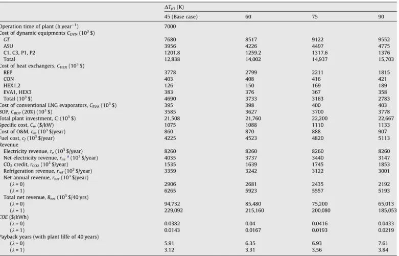
In the following calculation, the assumptions are kept un-changed as shown inTable 2, except the pinch point temperature differences, 45 K of DTp1in recuperator and 8 K of DTp2in CO2

condenser.

4.1. Effect of the pinch point temperature differenceDTp1in the recuperator REP

4.1.1. Effect ofDTp1on the cycle thermal performance

With the same net power outputWnetof 20 MW, simulation

computation is made of the basic cycle for values ofDTp1from 45 K to 90 K. The heat exchanger transfer area estimation and the cycle thermal performance are shown inTables 4 and 5. It should be pointed out that the heat transfer area estimation here is rough and based on the assumption that the heat exchangers are of the shell-and-tube type, and using average typical overall heat transfer coefficient values for these heat exchangers and fluids as found in the process heat transfer literature[38]. The recuperator REP is a conventional gas-to-gas heat exchanger; the heat exchanger HEX1 is also a gas-to-gas exchanger, HEX2 is a heat exchanger with phase change of gas-to-liquid in the hot side (16–17), and of LNG (containing some noncondensable gas) vaporizing in the cold side (19b–20b). The condenser CON consists of two parts, in the first part cooling of the CO2gas by the colder natural gas, followed by

the second part in which CO2is then condensed due to cooling

by liquid, boiling and gaseous natural gas, with an overall heat transfer coefficient of 600 W/m2_{K; the hot stream in EVA1 and}

HEX3 is assumed to be water with the inlet and outlet tempera-tures of 25 and 20°C, respectively.

As shown inTable 4, asDTp1is increased from 45 K to 90 K, the heat dutyQof the REP keeps decreasing and thus the heat transfer areaA of the REP decrease too although they are always higher than those in the other heat exchangers.Fig. 3explains the reason of the heat duty change in the REP: the hot side inlet temperature

t10is maintained fixed because of the fixed turbine inlet tempera-turet9and pressure ratiop9/p10, and the cold side inlet tempera-ture t6. The DTp1 always appears on the hot end of REP irrespective of its changes in this analysis. Hence, looking at

Fig. 3, thet7decreases and thetllincreases. As a result, theDTp1

temperature changes lead to the heat duty changes in the REP de-spite the mass flow rate increase of the working fluid in it.

Table 4indicates the heat transfer areaAin REP is reduced by 52% (or, by 8047 m2_{) as theDTp1is increased from 45 K to 90 K;}

while the total heat transfer area of all heat exchangers in the sys-tem,RA,is reduced by 30% (7483 m2_{), which is less than the}

de-crease for REP alone because the inde-crease of DTp1causes some increase in the LNG evaporation unit area.

Table 5indicates that the increase ofDTp1causes the increase of work input/output of the dynamic equipment (pumps P1 and P2, compressors C1 and C3, gas turbine GT). This is because the in-crease ofDTp1leads to the decrease of the inlet temperature of

combustorB(t7) as shown in Fig. 3, causing more fuel input to the combustor, and thus the working fluid flow rate going through

Table 3

Equipment and product cost information.

Equipment Price Equipment Price (103

$/m2 ) ASU 1376103_{$/(kg O} 2/s) Recuperator 0.244 O2compressor C1 164.5103$/(kg/s) Condenser 0.097 Compressor C3 164.5103 $/(kg/s) Heat exchangers 0.097 LNG pump P2 3.44103 $/(kg/s) Evaporator EVA1 0.097 CO2pump P1 3.2103$/(kg/s)

Product Price Product Price ($/kW h)

Fuel 0.197 $/N m3 _{Electricity 0.059}

CO2tax 0.033103$/(ton CO2) Refrigeration 0.059

1

Zorya–Mashproekt State Enterprise Gas Turbine Research & Production Complex, Ukraine.

the dynamic equipments increases (while the pressure changes across them remain the same).

We then examine the refrigeration output from the evapora-tors EVA1 where the low temperature liquid CO2 is evaporated,

and from HEX3 where the low temperature NG is heated to the near environment temperature. As theDTp1is increased,Table 5

shows that the cooling capacity and refrigeration exergy in the evaporator EVA1 increase, and that is entirely because of the asso-ciated increase in the liquid CO2mass flow rate, since the

refrig-eration temperature range is maintained fixed. Things are different in the HEX3: as theDTp1increases, both the HEX3 inlet temperature t21 and the LNG flow rate increase, and these two factors have opposite effects on the refrigeration output. The cal-culation results indicate that the negative effect of the former one dominates so overall that the refrigeration production in HEX3 de-creases. It can be seen from Table 5 that the reduction of refrigeration output in HEX3 surpasses the increment in EVA1, so there are reductions of 10.7% (6.1 MW) in the total cooling

Table 4

Estimation of heat transfer areas,A, for differentDTp1.

DTp1(K) Unit Q(MW) LMTD (K) U (W/m2K) A(m2) A(%) RA(m2)

45 (Basic case) Recuperator REP 74.17 51.5 93 15,487 62.2 24,892

LNG evaporation unit CON 44.81 29.6 99/600 4159 16.7

HEX1 9.75 77.2 99 1275 5.1

HEX2 0.9 55.9 600 27 0.1

Evaporation unit EVA1 42.42 33.6 429 2943 11.8

HEX3 14.51 33.8 429 1001 4

60 Recuperator REP 72.77 68.2 93 11,473 54.4 21,097

LNG evaporation unit CON 45.14 29.6 99/600 4205 19.9

HEX1 12.1 81.1 99 1507 7.1

HEX2 0.96 39.7 600 40 0.2

Evaporation unit EVA1 42.68 33.6 429 2961 14

HEX3 12.27 31.4 429 911 4.3

75 Recuperator REP 71.37 84.7 93 9060 48 18876

LNG evaporation unit CON 45.49 29.3 99/600 4286 22.7

HEX1 14.49 85.1 99 1720 9.1

HEX2 1.02 77.6 600 22 0.1

Evaporation unit EVA1 42.95 33.6 429 2980 15.8

HEX3 9.95 28.7 429 808 4.3

90 Recuperator REP 69.95 101.1 93 7440 42.7 17,409

LNG evaporation unit CON 45.83 29.3 99/600 4336 24.9

HEX1 16.9 89 99 1919 11

HEX2 1.08 71.4 600 25 0.1

Evaporation unit EVA1 43.23 33.6 429 2999 17.2

HEX3 7.64 25.8 429 690 4

Table 5

Cycle thermal performance for differentDTp1.

DTp1(K)

45 (Basic cycle) 60 75 90

Net power output,Wnet(MW), kept constant 20 20 20 20

Heat duty (MW) REP 74.17 72.77 71.37 69.95

CON 44.81 45.14 45.49 45.83 HEX1,2 10.65 13.06 15.51 17.98 Work (MW) Wlossa 0.831 0.832 0.833 0.834 WASU 2.338 2.493 2.654 2.817 P1 0.269 0.271 0.272 0.274 P2 1.906 1.918 1.93 1.942 C1 0.924 0.985 1.049 1.114 C3 0.264 0.282 0.3 0.318 GT 26.533 26.781 27.038 27.299 Refrigeration

EVA1 Temperature range (°C) 49.4 to 8 49.4 to 8 49.4 to 8 49.4 to 8

Cooling capacity (MW) 42.42 42.68 42.95 43.23

Exergy (MW) 6.57 6.61 6.66 6.67

HEX3 Temperature range (°C) 34.7 to 8 29.3 to 8 23.1 to 8 16.4 to 8

Cooling capacity (MW) 14.51 12.27 9.95 7.64

Exergy (MW) 2.387 1.844 1.363 0.95

Total cooling capacity,QC(MW) 56.94 54.95 52.90 50.87

Total exergy,EC(MW) 8.96 8.46 8.02 7.65

Mass flow rate (kg/s) Main working fluid,mwf 101.61 102.23 102.88 103.54

Retrieved liquid CO2,mco2,rec 1.846 1.971 2.098 2.228

NG fuel,mfuel 0.688 0.735 0.783 0.831

LNG,mLNG 95.54 96.122 96.735 97.356

Thermal efficiency,ge(%) 59.1 55.3 51.9 48.9

Exergy efficiency,h(%) 39.8 37.7 36.0 34.2

capacity QC, and of 14.6% (1.3 MW) in the total refrigeration exergy outputEC.

Fig. 4shows that the increase ofDTp1is unfavorable for the cy-cle efficiencies. AsDTp1is increased from 45 K to 90 K, the thermal

efficiency

g

and the exergy efficiencyhdeclines from 39.8% to 34.2%, a reduc-tion of 14.1%.

4.1.2. Effect ofDTp1on the cycle economic performance

Based on the cycle thermal performance results shown inTable 5, an economic analysis of the effect ofDTp1on cycle economic per-formance, including the system specific costCw, cost of electricity COE, payback periodPY, total net revenueRnet, etc., is performed

and the results are summarized inTable 6with the assumption of 40 years of plant lifeLp, 7000 of annual operation hoursHand

20 MW of net cycle power outputWnet.

The results of the economic analysis are shown inTable 6and

Figs. 5–9, and the following conclusions are drawn:

IncreasingDTp1from 45 K to 90 K indeed results in a reduction of 40.7% (1,907,000 $) in the cost of heat exchangers CHEX

mainly due to the decrease in the heat transfer areas, but also results in a counterproductive increase of 22.3% (2,865,000 $) in the cost CDYNof the dynamic equipment among which the

increase of gas turbine cost is caused by the increase of WGT

and the decrease of

g

of the other equipment’s cost is caused by the increase of work-ing fluid flow rate. Overall, that increase ofDTp1causes a 5.4% increase (1,159,000 $) in the total plant investmentCi, and thus

the related O&M cost increases by 47,000 $/year. Increasing

DTp1also increases the annual fuel cost by 21% (888,000 $/ year).

The system revenue is composed of three parts: (i) the CO2

creditrCO₂that is the revenue due to the reduction of CO2emission;

one of the most important characteristics of this cycle is zero-CO2-emission which enables the power plant to benefit from CO2

emission allowance trading. Since more fuel is consumed asDTp1

increases from 45 K to 90 K, more CO2is produced and retrieved,

therefore, the related revenue also increases by 20.7%, 318,000 $/ year; (ii) the electricity revenue re remains unchanged because

the net power output is assumed to be fixed as 20 MW for all val-ues ofDTp1increases, but here we prefer to use the net electricity revenuernewhich is defined as the electricity revenuerereduced

by the fuel cost cf, which in total shows a reduction of 22%,

888,000 $/year totally due to the increment of the fuel cost; (iii) the actual refrigeration revenuekrrefdepends on the refrigeration

market availability extent expressed bykthat can assume any va-lue between 0 and 1.Table 6shows that the upper limit (k= 1) of refrigeration revenuerrefis reduced by 10.7%, 358,000 $/year.

Based on the above analysis of cycle cost and revenue, the in-crease ofDTp1from 45 K to 90 K affects the specific costCw, total

net revenueRnet, cost of electricityCOEand payback periodPYas

follows:

(1) Specific costCwincreases. According to Eq.(4)andTable 6,

the 5.4% increase (1,159,000 $) in the total plant investment

Ci leads to and a 5.4% increase of Cw from 1075 $/kW to

1133 $/kW.

Since the actual refrigeration revenuekrrefvaries with the

value of the refrigeration revenue factork, we consider the total net revenueRnet, the cost of electricityCOEand the

pay-back periodPY, respectively, as a function of the refrigera-tion revenue factor k as well as of the pinch point temperature differenceDTp1. So the following analysis will discuss not only the effects ofDTp1and but also the effects in two extreme cases ofk= 0 andk= 1.

(2) Cost of electricityCOEincreases. According to Eqs. (5)–(7)

and Table 6, as DTp1 increases from 45 K to 90 K: (i) for

k= 0, the resulting increase of the sum of all the cost (bCi+cm+cf) surpasses the increase of the CO2creditrCO2,

and the cost of electricityCOEthus increases by 13.4%; (ii) for k= 1, the refrigeration revenue rref decreases with the

increase of DTp1, causing that the reduction of (rCO2+rref)

surpasses the increase of (bCi+cm+cf), and the cost of

elec-tricityCOEthus increases by 53.1%.

(3) System payback period PYis prolonged. Table 6 indicates that the annual valueBdecreases and the total plant invest-mentCiincreases, and therefore (Eq.(8)): (i) fork= 0, the

system payback period PY increases from 5.91 years to 7.61 years and (ii) fork= 1, thePYincreases from 3.12 years to 3.84 years.

(4) Total net revenueRnetdecreases. According to Eq. (10)for Rnet, the reduction of the net annual revenuernetand increase

of the total plant investment Ci in a reduction of 31.4%

(29,719,000 $/40 years) for k= 0, and 19.2% (44,039,000 $/ 40 years) fork= 1. -10 0 10 20 30 40 50 60 70 80 ΔTp1=45K ΔTp1=60K ΔTp1=75K

Q(MW)

t (

C)

Fig. 3.t–Qdiagram in REP for differentDTp1.

40 50 60 70 80 90 32 36 40 44 48 52 56 60 θ ηe Δ

T

(K)

,

(%)

It is thus concluded that the increase of theDTp1from 45 K to 90 K has negative effects on the cycle economic performance and makes it obvious that the optimal design in the considered range of parameters is at the lowest practicalDTp1= 45 K originally as-sumed in the system development.

It was also found that, for the sameDTp1, the system has a much better economic performance fork= 1 than fork= 0: the total net revenueRnetis 142% higher,COEis 50% lower, andPYis shortened

by at least 2.8 years.

4.2. Effect of the pinch point temperature differenceDTp2in the CO2 condenser CON

Among the needed heat exchangers, second to the size of the recuperator REP is the CO2 condenser CON. In the following

section, a sensitivity analysis is made of the thermal and economic

Table 6

Economic estimation for differentDTp1.

DTp1(K)

45 (Base case) 60 75 90

Operation time of plant (h year1

) 7000

Cost of dynamic equipmentsCDYN(103$)

GT 7680 8517 9122 9552

ASU 3956 4226 4497 4775

C1, C3, P1, P2 1201.8 1259.2 1317.6 1376

Total 12,838 14,002 14,937 15,703

Cost of heat exchangers,CHEX(103$)

REP 3778 2799 2211 1815 CON 403 408 416 421 HEX1,2 126 150 169 189 EVA1, HEX3 383 376 367 358 Total (103 $) 4690 3733 3163 2783

Cost of conventional LNG evaporators,CEVA(103$) 395 398 400 403

BOP,CBOP(20%) (103$) 3585 3627 3700 3778

Total plant investment,Ci(103$) 21,508 21,760 22,200 22,667

Specific cost,Cw($/kW) 1075 1088 1110 1133

Cost of O&M,cm(103$/year) 860 870 888 907

Fuel cost,cf(103$/year) 4225 4523 4820 5113

Revenue

Electricity revenue,re(103$/year) 8260 8260 8260 8260

Net electricity revenue,rnea(103$/year) 4035 3737 3440 3147

CO2credit,rCO2(103$/year) 1535 1639 1745 1853

Refrigeration revenue,rref(103$/year) 3359 3242 3122 3001

Net annual revenue,rnet(103$/year)

(k= 0) 2906 2681 2435 2192

(k= 1) 6265 5923 5557 5193

Total net revenue,Rnet(103$/40 yrs)

(k= 0) 94,732 85,480 75,200 65,013

(k= 1) 229,092 215,160 200,080 185,053

COE($/kWh)

(k= 0) 0.0382 0.04 0.0416 0.0433

(k= 1) 0.0143 0.0167 0.0193 0.0219

Payback years (with plant lilfe of 40 years)

(k= 0) 5.91 6.35 6.93 7.61

(k= 1) 3.12 3.31 3.56 3.84

a

The net electricity revenue,rne, is defined as the sum of the electricity revenuereminus the fuel costcf.

40 50 60 70 80 90 5000 10000 15000 20000 25000 30000

Cost of dynamic equipments, C DYN

ΔT_p1(K)

C_EVA+C_BOP+C_HEX

Total plant investment C_i Fuel cost,C_f

Cost of O&M,C_m Cost (103$)

Fig. 5.Effect ofDTp1on cycle costs.

40 50 60 70 80 90 0 2000 4000 6000 8000 10000 12000 14000 CO₂ credit, r_CO2 ΔT_p1(K) Revenue (103 $/year)

Refrigeration revenue, r_ref

Electricity revenue, r_e

effect of the pinch point temperature differenceDTp2in CON.DTp1

in REP is fixed at its near-optimal value of 45 K, and other main assumptions, including the turbine inlet/outlet parameters and the CO2 condensation pressure/temperature are maintain

unchanging as in the basic cycle where the values were fixed at

DTp1= 45 K,DTp2= 8 K.

4.2.1. Effect ofDTp2on the cycle thermal performance

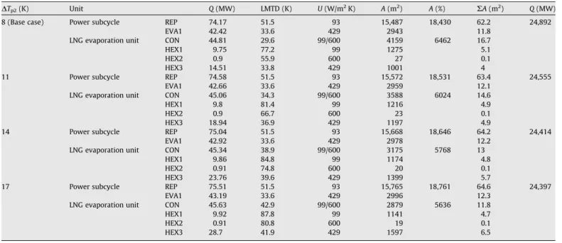
With the same net power outputWnetof 20 MW, simulation cal-culations are made to the basic cycle as theDTp2is varied from 8 K (the practical minimum, used in the basic cycle) to 17 K.Tables 7 and 8show the heat exchanger transfer area estimation and the cy-cle thermal performance under differentDTp2, respectively.

Fig. 10is thet–Qdiagram of CON, it can be seen that the heat duty of CON rises by 1.8% (0.82 MW) as theDTp2is raised from 8 K to 17 K. As assumed in the basic case, all the inlet and outlet temperatures (t13,t14andt19a) of CON, except the cold side outlet temperaturet20a, are maintained fixed as the DTp2is increased, so the increase ofDTp2is accomplished only by the decrease of

t20a. This moves the hot side stream temperature curve to the right, and the mass flow rate of the working fluid and the LNG through

the CON increase as well, therefore the heat duty of CON increases. At the same time, the mass flow rate of the working fluid and the LNG through the other heat exchangers will increase as well, leading to the increase of heat duties in all the heat exchangers as shown inTable 7.

Although the heat duties of all the heat exchangers rise with the increase ofDTp2, the heat transfer areas vary in completely differ-ent ways. As shown in Table 7, the heat transfer areas of heat exchangers REP and EVA1 (in the power subcycle) rise asDTp2 in-creases, because their LMTD-s remain unchanged while their heat duties increase. For the heat exchangers CON, HEX1,2 and HEX3, their heat transfer areas decrease asDTp2increases because their LMTD-s and heat duties increase but the LMTD-s increase more than the heat duties. The heat transfer area decrease in the LNG evaporation unit dominates over the area increase in the power subcycle, with a subsequent overall reduction of 2% (500 m2) in the total areaRAasDTp2is increased from 8 K to 17 K.

Fig. 11illustrates the effect ofDTp2on the thermal efficiency

g

and exergy efficiencyh. As theDTp2increases from 8 K to 17 K, the working fluid mass flow rate increases and the cycle specific power decreases. As a result, the net power output remains the same (20 MW), at the same time 1.9% (0.6 MW) more fuel energy input is required in the combustor B, and therefore the

g

1.8%. Also, more LNG flows through the cycle and thus 22% (8.2 MW) more LNG exergy is consumed and 43% (3.9 MW) more refrigeration exergy is produced, so the sum of exergy outputs is increased by 13.4% and the sum of exergy inputs is increased by 12%. As a result, the exergy efficiencyhhas a 1.2% increase.

4.2.2. Effect ofDTp2on the cycle economic performance

Based on the simulation results shown inTables 7 and 8, an analysis of the economic effect ofDTp2was performed and the cy-cle economic performance for differentDTp2is summarized in Ta-ble 9. The main assumptions are plant life Lp= 40 years, annual

operationH= 7000 h, and net cycle power outputWnet= 20 MW. Table 9andFigs. 12–16indicate the economic effects of increas-ingDTp2from 8 K to 17 K, as follows:

As shown inFig. 12andTable 9, there is little effect on the cost of heat exchangers CHEX, but it results in an increase of 3.7% (476,000 $) in the costCDYNof the dynamic equipment because of the increase of the working fluid flow rate. Overall, that increase ofDTp2causes a 3.1% increase (667,000 $) in the total plant investmentCi, and thus the related O&M cost increases

by 27,000 $/year. Increasing DTp2also causes the annual fuel cost to increase by 1.9% (79,000 $/year).

40 50 60 70 80 90 60000 90000 120000 150000 180000 210000 240000 λ = 0 ΔT_p1(K) R net(10 3 $/40 years) λ = 1

Fig. 7.Effect ofDTp1on total net revenueRnet.

40 50 60 70 80 90 0.015 0.020 0.025 0.030 0.035 0.040 0.045 λ=1 ΔT_p1(K) COE ($/kWh) λ=0

Fig. 8.Effect ofDTp1on the cost of electricityCOE.

40 50 60 70 80 90 3 5 7 λ=1 ΔT p1(K) PY(years) λ=0

Fig. 13andTable 9show the cycle revenue, which is composed of three parts: (i) the CO2creditrCO2; since more fuel is consumed

asDTp2increases, more CO2is produced and retrieved, therefore,

the related revenue also increases by 1.8%, or 28,000 $/year; (ii) the electricity revenuereremains unchanged because of the fixed

net power output, but the net electricity revenueredrops by 2%,

or 79,000 $/year, entirely due to the increase of the fuel cost. Apparently, the reduction in the electric power revenue is much higher than the revenue increase due to zero-CO2 emission; and

(iii) the refrigeration revenue krref; the upper limit (k= 1) of

refrigeration revenue rref increases by 26.3%, 883,000 $/year,

mainly because an increase of 98%, 14.2 MW, in the refrigeration cooling capacity in the HEX3 caused by the increase of the LNG mass flow rate from 95.5 kg/s to 116.2 kg/s and the drop of the in-let temperaturet21from35°C to50°C.

Consequently, the effects of increasingDTp2from 8 K to 17 K on

the specific costCw, the total net revenueRnet, the cost of electricity COEand the payback periodPYis as follows:

Table 7

Estimation of heat transfer area,A, for differentDTp2.

DTp2(K) Unit Q(MW) LMTD (K) U(W/m2K) A(m2) A(%) RA(m2) Q(MW)

8 (Base case) Power subcycle REP 74.17 51.5 93 15,487 18,430 62.2 24,892

EVA1 42.42 33.6 429 2943 11.8

LNG evaporation unit CON 44.81 29.6 99/600 4159 6462 16.7

HEX1 9.75 77.2 99 1275 5.1

HEX2 0.9 55.9 600 27 0.1

HEX3 14.51 33.8 429 1001 4

11 Power subcycle REP 74.58 51.5 93 15,572 18,531 63.4 24,555

EVA1 42.66 33.6 429 2959 12.1

LNG evaporation unit CON 45.06 34.3 99/600 3588 6024 14.6

HEX1 9.8 81.4 99 1216 4.9

HEX2 0.9 66.7 600 23 0.1

HEX3 18.94 36.9 429 1197 4.9

14 Power subcycle REP 75.04 51.5 93 15,668 18,646 64.2 24,414

EVA1 42.92 33.6 429 2978 12.2

LNG evaporation unit CON 45.34 38.9 99/600 3175 5768 13

HEX1 9.86 84.8 99 1174 4.8

HEX2 0.91 74.8 600 20 0.1

HEX3 23.76 39.6 429 1399 5.7

17 Power subcycle REP 75.51 51.5 93 15,765 18,761 64.6 24,397

EVA1 43.19 33.6 429 2996 12.3

LNG evaporation unit CON 45.63 42.9 99/600 2879 5636 11.8

HEX1 9.92 87.8 99 1141 4.7

HEX2 0.91 80.8 600 19 0.1

HEX3 28.7 41.9 429 1597 6.5

Table 8

Cycle thermal performance for differentDTp2.

DTp2(K)

8 (Base case) 11 14 17

Net power output,Wnet(MW) 20 20 20 20

Heat duty (MW) REP 74.17 74.58 75.04 75.51

CON 44.81 45.06 45.34 45.63 HEX1,2 10.65 10.7 10.77 10.83 Work (MW) Wloss 0.831 0.833 0.834 0.835 WASU 2.338 2.347 2.362 2.376 P1 0.269 0.27 0.272 0.273 P2 1.906 2.035 2.176 2.318 C1 0.924 0.928 0.933 0.939 C3 0.264 0.265 0.267 0.269 GT 26.533 26.678 26.843 27.01 Refrigeration

EVA1 Temperature range (°C) 49.4 to +8 49.4 to +8 49.4 to +8 49.4to +8

Cooling capacity (MW) 42.42 42.66 42.92 43.19

Exergy (MW) 6.57 6.61 6.65 6.69

HEX3 Temperature range (°C) 34.7 to +8 40.8 to +8 45.8 to +8 49.6to +8

Cooling capacity (MW) 14.51 18.94 23.76 28.7

Exergy (MW) 2.39 3.47 4.76 6.15

Total cooling capacityQC(MW) 56.94 61.6 66.68 71.89

Total exergyEC(MW) 8.96 10.08 11.41 12.84

Mass flow rate (kg/s) Main working fluid,mwf 101.61 102.17 102.8 103.43

Retrieved liquid CO2,mco2,rec 1.846 1.856 1.867 1.879

NG fuel,mfuel 0.688 0.692 0.696 0.701

LNG,mLNG 95.54 102 109.07 116.2

Thermal efficiency,ge(%) 59.06 58.73 58.37 58.01

(1) The specific costCwincreases: According to Eq.(4)andTable 9, the 3.1% increase (667,000 $) in the total plant investment

Ciresults in a 3.2% increase ofCw, from 1075 $/kW to 1109 $/

kW.

Again, the effects are considered for the limiting casesk= 0 andk= 1 in the following analysis.

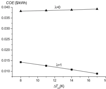
(2) Cost of electricity COE: According to the Eqs. (5)–(7)and

Table 9, asDTp2is increased from 8 K to 17 K: (i) fork= 0, the resulting increase of the sum of all the cost (bCi+Cm+ Cf) surpasses the increase of the CO2 credit rCO₂, and the cost of electricityCOEthus increases by 2.6%

Table 9

Costing estimation for differentDTp2.

DTp2(K)

8 (Base case) 11 14 17

Operation time of plant (h year1_{) 7000}

Cost of dynamic equipments,CDYN(103$)

GT 7680 7777 7883 7998

ASU 3956 3978 4003 4028

C1, C3, P1, P2 1201.8 1229 1258.5 1287.8

Total (103

$) 12,838 12,984 13,145 13,314

Cost of heat exchangers,CHEX(103$)

REP 3778 3800 3823 3847 EVA1 285 287 289 291 CON 403 348 308 279 HEX1,2 126 120 116 113 HEX3 98 116 136 155 Total (103 $) 4690 4671 4672 4685

Cost of the conventional LNG evaporatorsCEVA(103$) 395 422 451 480

BOP,CBOP(103$) 3585 3615 3654 3696

Total plant investment,Ci(103$) 21,508 21,692 21,922 22,175

Specific cost,Cw($/kW) 1075 1085 1096 1109

Cost of O&M,cm(103$/year) 860 868 877 887

Fuel cost,cf(103$/year) 4225 4250 4274 4304

Revenue

Electricity revenue,re(103$/year) 8260 8260 8260 8260

Net electricity revenue,rnea(103$/year) 4035 4010 3986 3956

CO2credit,rCO2(103$/year) 1535 1544 1553 1563

Refrigeration revenue,rref(103$/year) 3359 3634 3932 4242

Net annual revenue,rnet(103$/year)

(k= 0) 2906 2867 2824 2772

(k= 1) 6265 6501 6756 7014

Total net revenue,Rnet(103$/40 yrs)

(k= 0) 94,732 92,984 91,023 88,721

(k= 1) 229,092 238,344 248,302 258,401

COE($/kWh)

(k= 0) 0.0382 0.0385 0.0388 0.0392

(k= 1) 0.0143 0.0126 0.0108 0.0089

Payback years,PY(with plant life of 40 years)

(k= 0) 5.91 6.01 6.14 6.28

(k= 1) 3.12 3.06 2.97 2.9

a _{The net electricity revenue,r}

ne, is defined as the sum of the electricity revenuereminus the fuel costcf.

0 5 10 15 20 25 30 35 40 45 -170 -140 -110 -80 -50 -20 10 ΔTp2=8K ΔTp2=11K ΔTp2=14K Q (MW) t (O_C) ΔTp2=17K t 13a (constant) t₁₄ (constant) t_19a(constant) t_20a(decrease) Hot side Cold side

Fig. 10.t–Qdiagram of the condenser CON under differentDTp2.

8 10 12 14 16 18 39 42 45 48 51 54 57 60 ηe,θ (%) ΔTp2 (K) ηe θ

and (ii) for k= 1, it results in a 26.3% (883,000 $/year) increase in the refrigeration revenuerrefthat is the main

rea-son for a 37.8% reduction in the cost of electricityCOE. (3) System payback periodPY:Table 9shows that: (i) fork= 0,

the net annual revenuernetdecreases, thus prolonging the

system payback period PY from 5.91 years to 6.28 years according to Eq. (8); (ii) for k= 1, PY is shortened from 3.12 years to 2.9 years, mainly because of the increase in the annual valueBcaused by the increase in the refrigeration revenuerref.

(4) Total net revenueRnet: AsDTp2is increased from 8 K to 17 K:

(i) fork= 0, the reduction of the net annual revenuernetand

increase of the total plant investment Ci cause a 6.3%

(6,011,000 $/40 yrs) reduction in the total net revenueRnet

according to Eq. (10) and (ii) for k= 1, Rnet increases by

12.8% (29,309,000 $/40 yrs).

It is interesting to note from the above that increasing theDTp2

from 8 K to 17 K is unfavorable as evaluated byCOE,PYandRnetfor k= 0, while it is favorable fork= 1.

It was predicted, as shown inFigs. 14–16that, at the sameDTp2

the system economic performance is much better fork= 1 than for

8 10 12 14 16 18 5000 10000 15000 20000 25000 30000 Cost of O&M,C_m Fuel cost,C_f

Cost of dynamic equipments,C_DYN

ΔT_p2(K) Cost (103$)

C_EVA+C_BOP+C_HEX

Total plant investment, C_i

Fig. 12.Effect ofDTp2on cycle costs.

8 10 12 14 16 18 0 3000 6000 9000 12000 15000 ΔT p2 (K) Revenue (103$/year) CO 2 credit, rCO2 Electricity revenue, r_en Refrigeration revenue, r_ref

Fig. 13.Effect ofDTp2on cycle revenues.

8 10 12 14 16 18 70000 110000 150000 190000 230000 270000 λ=0 T_p2(K) R net (10 3_$/40years) λ=1

Fig. 14.Effect ofDTp2on total net revenueRnet.

8 10 12 14 16 18 0.010 0.015 0.020 0.025 0.030 0.035 0.040 λ=1 ΔTp2(K) COE ($/kWh) λ=0

Fig. 15.Effect ofDTp2on the cost of electricityCOE.

8 10 12 14 16 18 2 3 4 5 6 7 ΔTp2 (K) PY(years) λ=0 λ=1

k= 0: by a total net revenueRnetincrease over 142%, over 62%

de-crease in the cost of electricityCOE, and at least a 2.8 years shorter payback periodPY.

5. Conclusions

A thermoeconomic analysis was performed aimed at optimiza-tion of a novel power and refrigeraoptimiza-tion cogeneraoptimiza-tion system, COOLCEP-S, which produces near-zero-CO2 and other emissions

and has high efficiency. To achieve these desirable attributes, it uses the liquefied natural gas (LNG) coldness during its revaporiza-tion. In that, we focus on the study of the thermodynamic and eco-nomic effect of the pinch point temperature differences of the two most important heat exchangers,DTp1of the recuperator REP, and

DTp2of the CO2condenser CON in the COOLSEP-S system.

For the turbine inlet temperature of 900°C and pressure ratio of 4, cycle net power output of 20 MW, plant life of 40 years and 7000 annual operation hours, and two extreme cases of refrigeration revenue:k= 0 when this system has no financial benefit from the available refrigeration capacity andk= 1 when all the refrigeration produced in this plant can be sold for revenue.

The increase ofDTp1from 45 K to 90 K causes the following changes:

(1) The cycle thermal performance is worsened by a reduction of 17% in the thermal efficiency

g

efficiencyh.

(2) The cycle economic performance is worsened too: the spe-cific costCw increases by 5.4%, the cost of electricity COE

increases by 13.4% (k= 0) and by 53.1% (k= 1), the system payback period PYis prolonged by 1.7 years (k= 0) and

0.7 year (k= 1), the total net revenue Rnetis reduced by

31.4% (k= 0) and by 19.2% (k= 1).

The increase of DTp2 from 8 K to 17 K causes the following changes:

(1) The thermal efficiency

g

efficiencyhis increased by 1.2%. (2) The specific costCwincreases by 3.2%.

(3) Fork= 0, the cycle economic performance is worsened: the cost of electricityCOEincreases by 2.6%, the system payback periodPYis prolonged by 0.37 year, and the total net reve-nueRnetis reduced by 6.3%.

(4) Fork= 1, the cycle economic performance is improved: the cost of electricityCOEdecreases by 37.8%, the system pay-back periodPYis shortened by 0.22 years, and the total net revenueRnetincreases by 12.8%.

The resulting main recommendations are: (1) the optimal de-sign in the considered range of parameters is at the lowest practi-calDTp1= 45 K, (2) increasingDTp2is unfavorable forCOE,PYand

Rnet for k= 0, but favorable for k= 1, (3) for the same DTp1 or DTp2, the system has a much better economic performance for

k= 1 than for k= 0, (4) the cost of electricity in the base case (DTp1= 45 K, DTp2= 8 K) of this system is 0.0382 $/kWh (0.3 CNY/kWh) and the payback period is 5.9 years, much lower than those of conventional coal power plants being installed at this time in China, and yet COOLSEP-S has the additional major advan-tage in that it produces no CO2emissions.

Acknowledgements

The authors gratefully acknowledge the support from the Sta-toil ASA, and the Chinese Natural Science Foundation Project (No. 50520140517).

References

[1] Karashima N, Akutsu T. Development of LNG cryogenic power generation plant. In: Proceedings of 17th IECEC; 1982. p. 399–404.

[2] Angelino G. The use of liquid natural gas as heat sink for power cycles. ASME J Eng Power 1978;100:169–77.

[3] Kim CW, Chang SD, Ro ST. Analysis of the power cycle utilizing the cold energy of LNG. Int J Energy Res 1995;19:741–9.

[4] Najjar YSH, Zaamout MS. Cryogenic power conversion with regasification of LNG in a gas turbine plant. Energy Convers Manage 1993;34: 273–80.

[5] Wong W. LNG power recovery, proceedings of the institution of mechanical engineers. Part A: J Power Energy 1994;208:1–12.

[6] Deng S, Jin H, Cai R, Lin R. Novel cogeneration power system with liquefied natural gas (LNG) cryogenic exergy utilization. Energy 2004;29: 497–512.

[7] Krey G. Utilization of the cold by LNG vaporization with closed-cycle gas turbine. ASME J Eng Power 1980;102:225–30.

[8] Agazzani A, Massardo AF. An assessment of the performance of closed cycles with and without heat rejection at cryogenic temperatures. ASME J Eng Gas Turb Power 1999;121:458–65.

[9] Deng S, Jin H, et al. Novel gas turbine cycle with integration of CO2recovery and LNG cryogenic exergy utilization. In: Proceedings of ASME IMECE; 2001.

[10] Chiesa P. LNG receiving terminal associated with gas cycle power plants. ASME paper 97-GT-441; 1997.

[11] Desideri U, Belli C. Assessment of LNG regasification systems with cogeneration. In: Proceedings of TurboExpo 2000, Munich, Germany, 2000-GT-0165; 2000.

[12] Kim TS, Ro ST. Power augmentation of combined cycle power plants using cold energy of liquefied natural gas. Energy 2000;25:841–56.

[13] Velautham S, Ito T, Takata Y. Zero-emission combined power cycle using LNG cold. JSME Int J, Ser B. Fluids Therm Eng 2001;44: 668–74.

[14] Riemer P. Greenhouse gas mitigation technologies, an overview of the CO2 capture, storage and future activities of the IEA greenhouse gas R&D program. Energy Convers Manage 1996;37:665–70.

[15] Haugen HA, Eide LI. CO2capture and disposal: the realism of large scale scenarios. Energy Convers Manage 1996;37:1061–6.

[16] Jericha H, Gottlich E, Sanz W, Heitmeir F. Design optimization of the Graz cycle prototype plant. ASME J Eng Gas Turb Power 2004;126: 733–40.

[17] Anderson R, Brandt H, Doyle S, Pronske K, Viteri F. Power generation with 100% carbon capture and sequestration. In: 2nd Annual conference on carbon sequestration, Alexandria, VA; 2003.

[18] Marin O, Bourhis Y, Perrin N, Zanno PD, Viteri F, Anderson R. High efficiency, zero emission power generation based on a high-temperature steam cycle. In: 28th International technical conference on coal utilization & fuel systems, Clearwater, FL, USA; 2003.

[19] Mathieu P, Nihart R. Zero-emission MATIANT cycle. J Eng Gas Turb Power 1999;121:116–20.

[20] Mathieu P, Nihart R. Sensitivity analysis of the MATIANT cycle. Energy Convers Manage 1999;40:1687–700.

[21] Zhang N, Lior N. A novel near-zero CO2emission thermal cycle with LNG cryogenic exergy utilization. Energy 2006;31:1666–79.

[22] Zhang N, Lior N. Proposal and analysis of a novel zero CO2emission cycle with liquid natural gas cryogenic exergy utilization. J Eng Gas Turb Power 2006;128:81–91.

[23] Ishida M, Jin H. CO2 recovery in a novel power plant system with chemical-looping combustion. J Energy Convers Manage 1997;38(19): 187–92.

[24] Ishida M, Jin H. A new advanced power-generation system using chemical-looping combustion. Energy – Int J 1994;19:415–22.

[25] Griffin T, Sundkvist SG, Asen K, Bruun T. Advanced zero emissions gas turbine power plant. ASME J Eng Gas Turb Power 2005;27:81–5.

[26] Kvamsdal HM, Jordal K, Bolland O. A quantitative comparison of gas turbine cycles with CO2capture. Energy 2007;32:10–24.

[27] Zhang N, Lior N, Liu M, Han W. COOLCEP (cool clean efficient power): novel CO2-capturing oxy-fuel power systems with LNG (liquefied natural gas) coldness energy utilization, ECOS 2008. In: 21st Conference on efficiency, costs, optimization, simulation and environmental aspects of energy systems, vol. II, Krakow, Poland; 2008. p. 543–50.

[28] Liu M, Lior N, Zhang N, Han W. Thermoeconomic optimization of COOLCEP-S: a novel zero-CO2-emission power cycle using LNG (liquefied natural gas) coldness. In: ASME paper IMECE2008-6467, Proc. IMECE2008, ASME international mechanical engineering congress and exposition, Boston, Massachusetts, ASME, NY, November 2–6; 2008.

[29] Aspen PlusÒ

, Version 11.1, Aspen Technology, Inc.<http://www.aspentech. com/>.

[30] Lior N, Zhang N. Energy, exergy, and second law performance criteria. Energy – Int J 2007;32:281–96.

[31] Larson ED, Ren T. Synthetic fuel production by indirect coal liquefaction. Energy Sustain Dev 2003;VII(4).

[32] Kreutz T, Williams R, Consonni S, Chiesa P. Co-production of hydrogen, electricity and CO2from coal with commercially ready technology. Part B: Econ Anal Hydrogen Energy 2005;30:769–84.

[33] Jiaji Fu, Tong Yunhuan. Industrial economics. Beijing: Tsinghua University Press; 1996 [in Chinese].

[34]<http://www.wj.sh.cn/>[accessed October 2008]. [35]<http://www.kfas.com.cn/>[accessed October 2008]. [36]<http://www.cnjssw.com/>[accessed October 2008].

[37]<http://www.sunplushtech.com/low-temperature-pump.htm>[accessed Oct-ober 2008].

[38] Hewitt GF, Shires GL, Bott TR. Process heat transfer. Boca Raton: CRC Press/ Begell House; 1993.