Match Rates and Savings: Evidence from Individual Development Accounts

Match Rates and Savings:

Evidence from Individual Development Accounts

Mark Schreiner

June 2001

Microfinance Risk Management

6070 Chippewa St. #1W, St. Louis, MO 63109-3060, U.S.A. Telephone: (314) 481-9788, http://www.microfinance.com

and

Center for Social Development Washington University in St. Louis

Campus Box 1196, One Brookings Drive, St. Louis, MO 63130-4899, U.S.A.

JEL keywords: E21, Consumption and saving; J32, Private pensions; H3, Fiscal policy and household behavior

Abstract

How do people respond to matched-savings incentives? Studies of 401(k) plans find that matching increases participation but that higher match rates do not increase—and may decrease—the level of savings. This paper analyzes saving by low-income people in Individual Development Accounts (IDAs), a new savings incentive that matches withdrawals if used for home purchase, post-secondary education, or self-employment. The model controls for several sources of bias common in estimates of match-rate effects: unobserved heterogeneity among firms and among participants, censoring of savings at the match cap, and an inverse relationship between match rates and match caps. In IDAs, higher match rates are associated with an increased probability of continued participation but also with a decreased level of savings.

Acknowledgments

Michael Sherraden, Margaret Clancy, and Lissa Johnson helped with comments and with data collection and cleaning. Eleven foundations funded the American Dream Demonstration (ADD) of IDAs: Ford, Charles Stewart Mott, Joyce, F.B. Heron, John D. and Catherine T. MacArthur, Citigroup, Fannie Mae, Levi Strauss, Ewing Marion Kauffman, Rockefeller, and the Moriah Fund. Robert Friedman and the Corporation for Enterprise Development ran ADD. The views expressed here are mine.

1. Introduction

The federal government spends billions each year on tax breaks for Individual

Retirement Accounts (IRAs) and 401(k) plans. These incentives, however, are weak for

low-income people in low tax brackets. Individual Development Accounts (IDAs) are a

new savings incentive targeted to the poor (Sherraden, 1991). IDAs provide matches on

withdrawals for home purchase, post-secondary education, or self-employment. How do

people respond to the increased rate of return in this matched-savings structure?

For the level of savings, theory is ambiguous; the substitution effect and the

income effect work against each other. For participation, the income effect vanishes, so

higher rates of return should increase participation.

Empirical research takes two tacks. The first looks at the use of 401(k) plans

and/or IRAs and total savings. Perhaps one-third of contributions is new savings due

to incentives, with the strongest effects for low-income people (Engen and Gale, 2000;

Bernheim, 1997; Hubbard and Skinner, 1996). Conclusive measurement has been

thwarted by a lack of data on all assets and debts for people with exogenous differences

in access to savings incentives.

The second tack looks at rates of return for specific types of savings. The

empirical record suggests that household savings does not respond much (if at all) to

Deaton, 1992). Although the data preclude conclusive measurement, again effects seem

strongest for poor people (VanDerhei, Copeland, and Quick, 2000).

This paper takes this second tack; it looks at rates of return (match rates) and a

specific type of savings (IDAs). It avoids some (but not all) of the technical weaknesses

of past work on 401(k) plans.

Higher match rates are associated with an increased likelihood of continued

participation in IDAs. If the goal is to include more poor people in savings incentives,

then higher match rates worked. A higher match rate, however, was also linked with

decreased savings. This decrease might be real (income effects or target-saving effects)

or apparent (endogeneity of match rates and saving capacity). If the decrease was real

and if the goal was to boost aggregate personal savings, then higher match rates for

IDAs did not work; decreased savings more than offset increased participation. Even

though higher match rates decreased savings, they still boosted asset accumulation

(savings plus match). Thus, they may have facilitated the purchase of a big-ticket item

that might have led to discrete improvements in long-term well-being and capacity.

Section 2 describes IDAs. Section 3 reviews the measurement of match-rate

effects in the presence of match caps, endogeneity, unobserved heterogeneity, and

censoring. Section 4 presents the data, model, and results, and Section 5 discusses

2. Individual Development Accounts

Individual Development Accounts (IDAs) are matched-savings structures for the

poor. Withdrawals from IDAs are matched if used for home purchase, post-secondary

education, or self-employment. Participants also receive financial education and support

from peers and program staff. IDAs aim to include the poor in savings incentives, to

increase savings by the poor, and to boost ownership by the poor.

Sherraden (1988) proposed IDAs. The concept of asset-based policy has since

gained intellectual momentum (Shapiro and Wolfe, 2001; Ackerman and Alstott, 1999;

Conley, 1999; Stoesz and Saunders, 1999; Oliver and Shapiro, 1995). It has also

attracted broad political support. For example, IDAs are part of policy in most states,

and Bill Clinton proposed national IDA-like accounts. Both George W. Bush and Al

Gore had IDA proposals in their platforms, and a current bill (the Savings for Working

Families Act) would budget up to $10 billion for IDAs. The government of Canada will

sponsor an IDA demonstration in ten cities, and the government of the United Kingdom

has proposed IDA-like accounts.

IDAs are unique in that they are aimed at the poor, they subsidize

non-retirement savings, and they provide an explicit match. The rest of this section

compares and contrasts IDAs with Roth IRAs and 401(k) plans, two other common

1 _{Matches from employers in 401(k) plans are not subsidies but part of compensation.} 2 _{The Internal Revenue Service has not yet ruled on the tax status of IDA matches.}

Eligibility for IDAs is income-tested. Like Roth IRAs (which have universal

eligibility), deposits are supposed to come from earned income. Unlike 401(k) plans,

access and eligibility to IDAs are not provided through an employer.

Roth IRAs and 401(k) plans provide matches indirectly via tax breaks. Tax

deductions are worth little to poor people, so IDAs make direct matches. Matches in

IDAs are typically much higher than in 401(k) plans or Roth IRAs. Funds for IDA

matches and administrative expenses may come from private or public sources, whereas

the government pays for matches in Roth IRAs and 401(k) plans.1 _{Savers bear}

administrative expenses for Roth IRAs, and employers bear them for 401(k) plans.

IDAs are held in standard passbook savings accounts in banks, whereas Roth

IRAs and 401(k) plans are held in restricted-access accounts, often in mutual funds.

IDA deposits may be withdrawn at will and come from after-tax dollars (like Roth

IRAs but unlike 401(k) plans) and earnings are taxed (unlike Roth IRAs or 401(k)

plans).2 _{Withdrawals from IDAs for purposes other than home purchase, post-secondary}

education, or self-employment are not matched but are not otherwise penalized; early

distributions from Roth IRAs are subject to an excise tax, and early distributions from

3 _{IDAs and their subsidies for savings for asset purchases in the near term resemble a}

program that subsidized savings for a down payment on a home in Canada from 1974 to 1985. Unlike IDAs, the Canadian program matched through tax breaks, so most participants were in high tax brackets (Engelhardt, 1996).

IDAs—unlike Roth IRAs and 401(k) plans—are meant primarily for

pre-retirement asset purchases rather than pre-retirement consumption. This is the aspect in

which IDAs differ most from Roth IRAs and 401(k) plans.3

IDA programs (so far at least) are administered by not-for-profit organizations.

The not-for-profit sets the match cap, which may be annual or for a span beyond one

year. In contrast, 401(k) plans are sponsored by employers and have annual match caps

set by the employer and/or by law. Roth IRAs are administered by financial-service

organizations and have annual match caps set by law. Payroll deduction is required for

401(k) plans and is possible—but not required—for IDAs and Roth IRAs. Finally,

financial education is required in IDAs but is voluntary (if available) in 401(k) plans

4 _{Clancy (1996) does not explicitly say whether individual or firm data were used.}

3. Measurement of match-rate effects

The ideal test of the effects of match rates would measure participation, savings,

and all personal and program characteristics for people with exogenous differences in

match rates. No study (including this one) achieves the ideal. This section reviews past

work and argues that their estimates of match-rate effects are biased because they fail

to control for match caps, censoring, endogeneity, and unobserved heterogeneity.

3.1 Research on matched savings in 401(k) plans

Early studies of match rates use firm-level data. GAO (1988, cited in Poterba,

Venti, and Wise, 1994) tabulates participation and savings by match rate and find that

both outcomes increase with the presence of a match (perhaps at a decreasing rate) and

with the match rate. Neither study uses statistics nor controls for variables that might

cause spurious correlations between the match rate, participation, and/or savings.

Three other early studies use statistics with firm-level data. Correlation analysis

of employees who earned $32,000 a year or less at 24 firms in 1995 showed that

participation (but not savings) increased with the match rate (Clancy, 1996).4 _Papke,

Petersen, and Poterba (1996) and Papke and Poterba (1995) use regressions with one

5 _{The results are weakened because match rates are imputed from Form 5500 data.}

participation increases with matching. Papke and Poterba (1995) also find that higher

match rates—once there is a match—are not linked with savings.

These early studies point in one direction, but they use small samples, simple

methods, and firm-level data that may mask individual behavior. A second set of

studies uses larger samples, more control variables, and sometimes data on individuals.

3.1.2 Second-generation research

Papke (1995) uses pooled regressions with panel data on 3,565 to 5,363 firms

from 1985-1987.5 _{With higher match rates, participation increases (at a decreasing}

rate), and savings increase (at very low match rates) and then decrease. The effects on

diminish or vanish with controls for unobserved firm-level heterogeneity.

Bayer, Bernheim, and Scholz (1996) use a panel of 1,100 firms in 1993-94. In

pooled regressions with nine control variables, the presence of a match is linked both

with increased participation and increased savings. Again, the effects shrink or vanish

with controls for unobserved firm-level heterogeneity.

Andrews (1992) regresses participation and savings on the presence of a match

and on eleven other variables for 3,884 individuals from the May 1988 Employee

Benefit Supplement of the Current Population Survey (CPS). Matching is associated

Bassett, Fleming, and Rodrigues (1998) use the April 1993 CPS. Regression with

eight controls suggests that participation increases in the presence of a match but that

the level of the match rate does not matter. They also show simple tabulations in which

contribution rates decrease as match rates increase.

Clark and Schieber (1998) use regressions with five controls for 60,919 people at

19 firms in 1994. Higher match rates increase both participation and contributions.

Clark et al. (2000) use similar data for 156,376 people at 87 firms in 1995. They find

that higher matches increase participation but decrease contributions.

Munnell, Sundén, and Taylor (2000) use the 1998 Survey of Consumer Finances

(SCF). In a regression with 8 controls and 1,232 participants, matching is linked with

increased savings but, higher match rates are linked with decreased savings.

Like early studies, this second generation finds that the presence of a match

increases participation. With their improved data and technique, however, some find

that higher match rates do not increase—and may decrease—the level of savings.

3.1.3 Third-generation research

The best, most-recent studies use individual data, control for moderate numbers

of other variables, and account for match caps and/or possible endogeneity of match

rates with unconditional savings. On the whole, they still find that a match increases

Even and Macpherson (2001) use 1993 CPS data and control for 18 variables

and for the chance that firms with unconditionally low savers are more likely to

introduce matching (or to increase the match rate) to boost participation and savings.

Such endogeneity—if it exists—would tend to mask any positive effects of matching.

They find much larger match-rate effects on participation than in previous studies.

VanDerhei, Copeland, and Quick (2000) use the best data yet: characteristics for

137 plans and their 163,346 participants. Besides age, wage, and tenure, they control

for the match cap (although they do not interact it with the match rate). They find

that higher match rates are linked with decreased savings and that higher match caps

are linked with increased savings. This suggests, for example, that a total potential

match of 4 percent of salary would elicit more savings as a 50-percent match rate on up

to 8 percent of salary than as a 100-percent match rate on up to 4 percent of salary.

3.1.4 Summary

The best work on 401(k) plans suggests that the presence of a match increases

participation. Once there is a match, participation increases at a decreasing rate.

Higher match rates do not increase savings and may even decrease it.

That the presence of a match should increase participation and savings is not a

surprise; only the substitution effect is at work. That higher match rates would decrease

savings is theoretically possible—the result of income effects or target-saving—but is

6 _{In a 401(k) plan, the match rate is the number of dollars from the employer for each}

dollar from the employee. Tax breaks for 401(k) plans are equivalent to matches, even though they are not put in 401(k) plans. In this sense, research on 401(k) plans that ignore tax breaks understate the match rate. This study also ignores taxes, but most IDA participants are in low tax brackets; only people with income under 200 percent of poverty qualified for ADD, and the median participant was at the poverty line.

7 _{401(k) plans have up to two match caps. The employer matches contributions up to}

the employer-match cap, and the government gives tax breaks on contributions up to to control for censoring, endogeneity, unobserved heterogeneity, and/or the negative

correlation between match rates and match caps.

3.2 Match caps

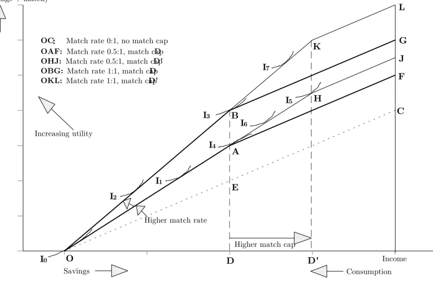
To show how match caps may affect estimates of match-rate effects, Figure 1

depicts budget sets for a person with an IDA. On the horizontal axis, savings increase

from left to right, and consumption increases from right to left. The vertical axis shows

asset accumulation (savings plus match). Utility increases to the northwest.

3.2.1 Match rates and match caps

In an IDA, the match rate is the number of dollars disbursed to a vendor for

each dollar withdrawn by the participant for a matchable purchase.6 _{In Figure 1, the}

match rate is the slope of the budget line minus unity, that is, 0:1 for OC, 0.5:1 for OA, and 1:1 for OB.

Match caps are limits on matchable deposits. IDAs cap the number of matchable

dollars, although participants are free to put non-matchable dollars in the same

the IRS match cap. Furthermore, specific plans may limit contributions at some point beyond the employer-match cap but before the IRS-match cap. Employer caps limit salary-deferral percentages, and IRS caps limit numbers of dollars.

8 _{Bernheim and Scholz (1993) suggest that target-saving predominates for poor people.}

Potential match Match cap Match rate . (1)

Potential asset accumulation Match cap Potential match ,

Match cap ( Match cap Match rate ) ,

Match cap ( 1 Match rate ) .

(2) 3.2.2 Potential matches and potential asset accumulation

The potential match is the product of the match cap and the match rate:

In Figure 1, the potential match (match rate 0.5:1, match cap D) is AE. A given potential match may result from a range of pairs of match rates and match caps.

For example, a $500 potential match may result from a 0.5:1 match rate with a $1,000

match cap or from a 1:1 match rate with a $500 match cap. In 401(k) plans, match

rates and match caps are negatively correlated (VanDerhei, Copeland, and Quick, 2000;

Clancy, 1996; Papke, Petersen, and Poterba, 1996).

Potential asset accumulation is the match cap plus the potential match:

In Figure 1, potential asset accumulation with a match rate of 0.5:1 and a

match cap of D is AD. Potential asset accumulation especially matters for target-savers. IDA participants plan to purchase a big-ticket item and so may be particularly

Together, match rates and match caps determine the potential match and

potential asset accumulation. Theory predicts two types of effects on participation and

savings due to changes in match rates and/or match caps: economic effects

(substitution and/or income), and behavioral effects.

3.2.3 Economic effects

The economic theory of matched-savings structures discussed below highlights

that the analysis of match-rate effects must control for variation in match caps.

3.2.3.1 Participation

Participation is all-or-none, so match rates exert only substitution effects. For

the example of a match rate of 0:1 (budget OC in Figure 1), the northwest-most indifference curve (I₀) is tangent to the budget at O; the person does not participate. As the match rate increases and the budget rotates up and left (first to 0.5:1 for OAF and then to 1:1 for OBG), the likelihood that the tangency will move off O (say, to I₁ or I₂) increases. Thus, higher match rates can only increase participation.

The match cap has no economic effects on participation. A shift from D to D´ (and the 0.5:1 budget from OAF to OHJ) does not change the slope near O, and quasi-concave utility implies that no tangencies on HJ give greater utility than at O. 3.2.3.2 Level of savings

The economic effects of changes in match rates (and/or changes in match caps)

9 _{If the indifference curve is exactly tangent to the budget at the original match}

cap—and this is unlikely—then a higher match cap will not increase savings. If savings are not at the match cap (say, at I1 with a match rate of 0.5:1 on

budget OAF), then an increase in the match rate has both income and substitution effects; either could dominate. For example, a move to a match rate of 1:1 on budget

OBG could lead to tangency at I₂ (decreased savings) or at I₃ (increased savings). If savings are not at the match cap, then the match cap has no economic effect.

For example, with tangency at I₁ with a 0.5:1 match rate and a match cap of D, a shift to a match cap of D´ (budget OAF to OHJ) leaves the optimal choice unchanged.

If savings are at the match cap (for example, I4 on budget OAF with a 0.5:1

match rate and a match cap of D), then a higher match rate has only an income effect. Savings may decrease (for example, to I₂) or stay the same (I₃).

If savings are at the match cap (say, I₄ at D on budget OAF), then a higher cap (D´ on budget OHJ) will increase savings (for example, to I₅ or I₆).9

3.2.3.3 How the match cap may confound estimates of match-rate effects The theory above looks at changes in either match rates or match caps, with the

other held constant. In 401(k) plans in practice, however, high match rates go with low

match caps (and inversely). If estimates of match-rate effects do not hold match caps

constant, then higher match rates may seem to decrease savings even if they really

10 _{This bias affects all who would save more at the lower match rate (0.5:1) and higher}

match cap (D´) than at the lower match cap (D) and higher match rate (1:1). The bias also affects all who, at the higher match rate (1:1), save up to the lower match cap (D). In practice, many participants save at the match cap, so the bias could be large.

For example, suppose that an increase in the match rate from 0.5:1 to 1:1 (with

the match cap of D´ held constant) would increase saving from I6 to I7 (Figure 1). If,

however, the higher match rate comes with a lower match cap D, then matched savings must decrease, say from I₆ to I₃. Failure to control for the match cap would show

(incorrectly) that higher match rates decrease savings.10

Estimates of match-rate effects should control for the match cap. Only

VanDerhei, Copeland, and Quick (2000) have done so. Estimates of the effects of match

rates on savings in other studies are biased downwards, perhaps severely.

3.2.4 Behavioral effects

Match rates and match caps can have behavioral effects because people lack

total rationality, complete information, and perfect imagination. The costs of

decision-making often lead to choices based on habit, culture, rules of thumb, or what public

policy seems to suggest. Saving may be particularly subject to these behavioral effects

(Beverly and Sherraden, 1999; Caskey, 1997; Thaler, 1994; Sherraden, 1991; Maital,

1986), in part because costs are swift and sure but rewards are distant and uncertain,

Furthermore, the human body evolved in a context of extreme scarcity and so may

have a bias for short-term gratification even at the expense of long-term well-being.

Bernheim (1999) discusses how the behavioral effects of savings incentives may

increase savings. Foremost, people may take the mere existence of incentives—be they

IDAs, IRAs, or 401(k) plans—as a suggestion that they can and should save. Likewise,

the existence of a match signals that saving is a good idea; without much in the way of

a personal benefit-cost analysis, people may assume that they would be fools not to

take advantage of “free money”. Furthermore, restrictions on the use of matched

savings may highlight goals (such as home ownership, college education, or retirement

security) that people might not focus on otherwise. People may also regard matched

savings (even if fully liquid, as in IDAs) as “off limits”, and this curbs temptations to

consume. Finally, people may turn match caps into goals and so may try to save more

if match caps are higher. In sum, behavioral theory predicts greater participation and

greater savings with higher match rates and with higher match caps.

Can behavioral effects be distinguished from economic effects? Only economic

(income) effects can explain decreases in participation and savings. If savings and/or

participation increase with higher match rates, however, the cause could be behavioral

or economic (substitution). The only sharp test involves changes in the match cap.

cap), but behavioral theory predicts changes in both participation and savings. Studies

on 401(k) plans have not distinguished between behavioral and economic effects.

3.3 Endogeneity

In 401(k) plans, match rates may depend on unconditional savings in two ways.

On the one hand, high savers may demand high match rates. On the other hand, firms

with low savers may introduce matching or boost match rates to fulfill

non-discrimination requirements. Estimates of match-rate effects are biased upwards by the

first type of endogeneity and downwards by the second type.

Only one paper convincingly controls for endogeneity. Even and Macpherson

(2001) find that firms do add matching or raise match rates in response to low

participation and/or low savings. Thus, estimates of match-rate effects that do not

account for endogeneity may be biased downwards.

3.4 Unobserved heterogeneity

Unobserved characteristics of firms or participants may be correlated both with

savings and with match rates. This unobserved heterogeneity could bias estimates of

match-rate effects either upwards or downwards.

The few studies of 401(k) plans that do deal with unobserved heterogeneity find

that firm-level controls weaken otherwise-positive associations between match rates and

participation and savings (Bayer, Bernheim, and Scholz, 1996; Papke, Petersen, and

11 _{Match caps censor desired savings, but the need to control for match caps is distinct}

from the need to control for censoring. Controlling for censoring is also distinct from controlling for kinks. Kinks affect estimates of the effects of matched-savings structures on total savings (Moffitt, 1990); this paper—and the 401(k) literature—look only at effects on matched savings.

3.5 Censoring

Even if desired savings responds to changes in match rates, actual savings may

change little or not at all, due to the match cap. Estimates of match-rate effects that do

not control for this censoring are attenuated toward zero.

For example, suppose that desired savings with a $500 match cap and a 1:1

match rate is $450. With a 2:1 match rate, desired savings may exceed the $500 cap.

Actual savings, however, is capped at $500, so the effect on actual savings is smaller

than the effect on desired savings.

This paper asks about effects on desired savings. This is the appropriate

question for counterfactual policy analysis. Given changes in desired savings, changes in

actual savings, given a specific match cap, are straightforward to compute.

How often do desired and actual savings diverge? In studies of specific 401(k)

plans, Kusko, Papke, and Poterba (1998) and Yakoboski and VanDerhei (1996) find

that about 20-30 percent of participants saved up to the highest match cap. In the

IDAs studied here, 26 percent of continuing participants were at the match cap. Thus,

3.6 Summary

Estimates of the effects of match rates should control for bias due to negative

correlations between match caps and match rates, censoring, endogeneity, and

unobserved heterogeneity among programs and among participants. No estimate in the

401(k) literature controls for more than one of these five possible sources of bias. This

4. Data, model, and results

The analysis here controls for match caps and for a wide range of characteristics

of programs and participants. It also addresses censoring and unobserved heterogeneity,

but not endogeneity. For IDAs examined here, higher match rates were associated with

increased continued participation but with decreased savings.

4.1 Data from the American Dream Demonstration

The American Dream Demonstration (ADD) comprises 14 IDA programs across

the United States. Enrollment started in July 1997, and 2,378 participants had opened

an IDA by June 30, 2000 (Schreiner et al., 2001).

Data on programs and participants in ADD come from management-information

software used by programs (Johnson, Hinterlong, and Sherraden, 2001). The system

records account-structure parameters, demographic and socio-economic data on

participants, and monthly IDA cash flows. The cash-flow data are accurate and

complete; they come from bank records, satisfy accounting identities, and were

extensively cross-checked. It may be the best (or only) high-frequency data on matched

savings by the poor.

4.1.1 Type of match-cap structure

Participants in ADD face either annual or lifetime match caps. Annual match

caps limit matchable dollars in a participation year. Lifetime match caps limit total

12 _{In practice, imperfect rationality may make match-rate effects stronger for continuing}

participation than for participation. Although opportunity costs are the same for exit Of the 2,378 participants in ADD, this paper analyzes the 807 who had an

annual match cap and who exited before the end of their first year or who completed at

least 12 months as of June 30, 2000. Participants are analyzed just after their twelfth

month for two reasons. First, like all other permanent-access matched-savings

structures, any permanent-access IDA would have an annual match cap, in part to

prevent abuse. Second, some participants in IDAs—as in IRAs—make large deposits

just before the deadline. Figure 2 shows that net deposits in ADD spike at year-end.

Measuring IDA savings before an annual or lifetime deadline would be like measuring

IRA savings in October even though most IRA deposits for a tax year are made before

April 15 in the next calender year.

4.1.2 Continued participation

There are no data on eligible people who choose not to participate in ADD, so

this paper cannot look at the effects of match rates on participation. Instead, it looks at

effects on continued participation through month 12 after enrollment. The opposite of

continued participation is exit, that is, leaving ADD without a matched withdrawal.

In theory, continued participation is analogous to participation; just as a

non-participant can enroll at any time, a non-participant can exit at any time. Opportunity

costs are the same for exit as for non-participation; factors that increase (decrease)

and for non-participation, participants may “feel” exit costs more than non-participants because participants are more likely to know what they are missing.

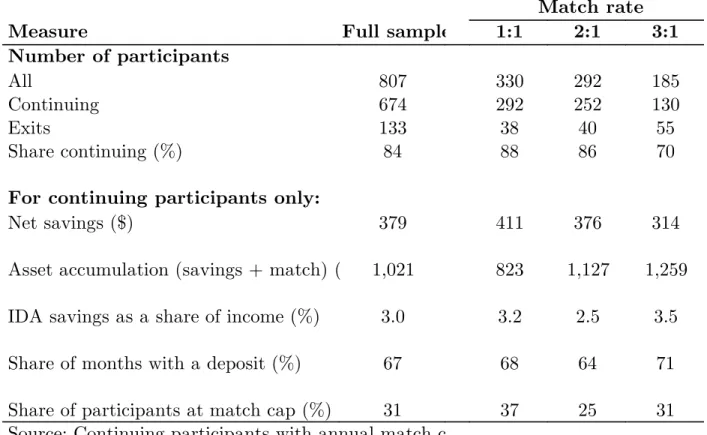
About 84 percent of participants continued participation through month 12

(Table 2). The share continuing was higher for match rates of 1:1 and 2:1 than for

match rates of 3:1. Theory cannot explain this, but the tabulations do not control for

other variables correlated both with continuing participation and with match rates.

4.1.3 Level of IDA savings

IDA savings are the smaller of the match cap or of deposits minus unmatched

withdrawals. Unlike research on 401(k) plans, this paper looks at savings in terms of

dollars rather than in terms of shares of income. This is because IDA match caps are in

terms of dollars and because income data in ADD are noisy.

Average net savings in the first 12 months were $379 (Table 2). Savings

decreased with the match rate: $411 for 1:1, $376 for 2:1, and $314 for 3:1. Again, the

tabulations do not control for other variables and so may not say much about

match-rate effects.

Table 2 also shows that asset accumulation (savings plus match) averaged

$1,021 and increased with the match rate. IDA savings as a share of income averaged

3.0 percent and was highest for 3:1 match rates. On average, continuing participants

4.1.4 Variation in match caps and match rates

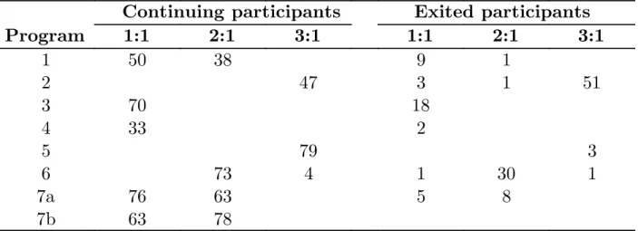
Match caps in ADD do not vary much (Table 3). This likely precludes reliable

estimates of match-cap effects.

Unlike match caps, match rates in ADD vary both between programs and within

programs both for continuing participants and for exited participants (Table 4). This

allows controls for both match rates and program-level unobserved heterogeneity.

4.1.5 Endogeneity

Two-way causation between the match rate and unconditional savings is the

main threat to validity in this study. Although participants could not choose among

IDA programs by their match rates (ADD was all there was), unconditional savings

may still be correlated with match rates in three ways.

First, programs often targeted specific groups, and they may have set higher

(lower) match rates if they expected to serve unconditionally low (high) savers

(Sherraden et al., 2000). This would bias the estimated match-rate effect downwards.

Second, Program 1 had a 1:1 match rate except for participants who received

Temporary Assistance for Needy Families (TANF); their match rate was 2:1. If TANF

receipt was correlated with unobserved characteristics that affect unconditional savings,

then linking match rates with TANF produces endogeneity bias. For example, if TANF

13 _{Schreiner et al. (2001) discuss the data from ADD at length.}

Third, Programs 7a and 7b gave a match rate of 2:1 to home buyers and 1:1 to

others. If home buyers were high savers, then the bias is upwards. If home buyers were

target-savers—for example, for a fixed down payment—then the bias is downwards.

The data provide no way to control for endogeneity where match rates depend

on expected savings. Dummies mark the receipt of public assistance and the intended

use of the IDA control for the other two types of endogeneity. These imperfect controls

are the best that the data allow. The paper returns to this issue below.

4.1.6 Data caveats

Of course, no data set is perfect, and four points are noted here.13 _{First, the}

demographic and socio-economic characteristics of participants are measured at

enrollment, but they may have changed afterwards. Second, despite a strong

commitment to evaluation by IDA staff, data quality varies among programs. Third,

participant income, assets, and debts are noisy and probably understated, as in most

surveys. Fourth, continued participation may be overstated because participants may

exit de facto even if the program has not marked them as exits.

4.2 Model

With data on a wide range of program and participant characteristics, this paper

uses a Tobit model with selection for continued participation to control for match caps,

zi w_i u_i. (3)

y_i x_{i i}. (4)

The first step is a Probit for continued participation. For person i, z*_{i is the}

desire to participate through month 12. Desire to continue is assumed to be a linear

function of a vector wi of independent variables and an error term ui:

The controls w_i include a set of dummies for the match rate (with 1:1 omitted), a single variable for the match cap, and a set of program dummies to control for

program-level heterogeneity. Appendix A describes other independent variables.

Desired continued participation z*_{i is unobserved. Actual continued participation}

d_i is observed, and it equals unity if z*_{i is positive and zero otherwise.}

The second step is a Tobit with savings censored at the match cap (31 percent of

continuing participants are censored, Table 2). In standard Heckman fashion, a

transformation of the error term from the first-step Probit becomes, in the second-step

Tobit, a control for unobserved individual heterogeneity that affects both the likelihood

of continued participation and the level of savings for continuing participants. Desired

savings y*_{i is a linear function of independent variables x}

Observed savings y_i equals the smaller of desired savings y*_{i or the match cap. As}

in the first-step Probit, the controls x_i include dummies for the match rate, a variable for the match cap, and dummies to control for program-level unobserved heterogeneity,

as well as the transformed Probit error term to control for individual-level unobserved

heterogeneity. The error terms u and are bivariate normal with correlation .

4.3 Results

Maximum-likelihood estimates for the Tobit model with sample selection are

presented below for the match cap and match rate. Other results are in Appendix A.

The estimated correlation is positive, large (0.56), and statistically significant (p = 0.01, Table A5). Unobserved characteristics that make a participant more likely to

continue participation also serve to increase desired savings.

4.3.1 Match caps

Consistent with economic theory (but not with behavioral theory), the match cap

was not associated with continued participation in IDAs in ADD (Table 5). An increase

in the match cap of $100 is estimated to decrease the likelihood of continued

participation by 0.04 percentage points, and the p-value of the coefficient is high (0.29).

Expected desired savings decreased by $74 for each $100 increase in the match

For two reasons, both of these results are probably peculiar to this data set.

First, match caps vary little, both between programs and within programs. Second,

neither economic nor behavioral theory can explain negative match-cap effects.

4.3.2 Match rates

Higher match rates for IDAs in ADD were associated with a greater likelihood of

continued participation. The estimated changes are 0.35 percentage points for the move

from 1:1 to 2:1 and 0.87 percentage points for the move from 1:1 to 3:1 (coefficient

p-values are 0.04, Table 5). These effects are small compared with the large changes in

the match rate. This paper cannot test for the importance of the presence of a match,

but perhaps continued participation in IDAs—as research has found for 401(k)

plans—depends more on the presence of a match than on the match rate.

Higher match rates decreased desired savings (Table 5). The move from 1:1 to

2:1 was associated with a reduction of $102 (p = 0.02). The move from 1:1 to 3:1 was

associated with a reduction of $232, but the coefficient was not statistically significant

(p = 0.59). In ADD, income and/or target-saving effects swamped substitution effects.

To recap, higher match rates increased participation a little and decreased

desired savings a lot.

4.3.3 Asset accumulation

Do higher match rates increase or decrease asset accumulation (savings plus

participants, predicted desired savings averages $518. With a 2:1 match rate, the

average is $416. Asset accumulation is then $1,036 at 1:1 and $1,248 at 2:1. Thus,

decreased savings would offset some—but not all—of the effects of a higher match rate

on asset accumulation.

In the presence of match caps, the offset is smaller because some of the decrease

in desired savings does not affect actual savings because it takes place above the caps.

For example, with a match rate of 1:1 for all continuing participants, average predicted

savings with the match caps in ADD is $468 (asset accumulation of $936); with a

match rate of 2:1, average predicted savings is $392 (asset accumulation of $1,176).

4.3.4 Bias in past estimates of match-rate effects

This paper addresses some sources of bias ignored in most research on 401(k)

plans. Did this care with match caps, censoring, and unobserved heterogeneity matter?

To check, a Tobit with sample selection was run without a variable for the

match cap. As might be expected—given that the match cap varies little in this

data—effects were unchanged, except the estimate for a 3:1 match rate on desired

savings fell to less than $1 (p = 0.92).

Without program dummies, results change drastically. Match rates of 2:1 no

longer affect participation, and match rates of 3:1 decrease participation. Desired

for match rates of 3:1 compared with 1:1 (p = 0.40). The results without controls for

program-level unobserved heterogeneity do not make much sense.

A Probit and a Tobit were run separately to check whether individual

heterogeneity mattered. Participation results were virtually unchanged. The

desired-savings regression, however, had match-rate effects of essentially zero. This is unlikely.

Censoring also mattered. First-step results for a selection model with ordinary

least-squares in the second step (rather than a Tobit) were virtually unchanged. As

expected, match-rate effects on desired savings were attenuated toward zero, $74 for 2:1 match rates and $181 for 3:1 match rates.

Controls for match caps, censoring, and unobserved heterogeneity did matter,

especially for effects on desired savings. Although IDAs are not exactly like 401(k)

plans, the measurement issues are quite similar, so the usefulness of work on

match-rate effects in 401(k) plans that do not control for these sources of bias is unclear.

Finally, although the model here controls for many sources of bias, it cannot

control for all possible forms of endogeneity between match rates and unconditional

savings. This weakens the robustness of the results. IDA programs in ADD may have

set match rates higher (lower) if they expected participants to be low (high)

unconditional savers. This biases estimates of match-rate effects downwards, so the

5. Discussion

For IDAs in ADD, higher match rates were linked with increased participation

but with decreased savings. Higher match rates may have income effects that swamp

substitution effects, and/or people with IDAs may target-save. Endogeneity between

the match rate and unconditional savings may also explain at least part of the effect.

What does this mean for policy? The response of savings to match rates matters

because of cost. The government spends billions each year on tax breaks for IRAs and

401(k) plans, and IDAs cost even more per dollar saved, both because of higher match

rates and because of higher administrative costs (Schreiner et al., 2001).

IDA policy might have three (not necessarily exclusive) goals. The first is to

include more poor people in savings incentives (Sherraden, 2001). For IDAs in ADD,

higher match rates increased participation and thus served this purpose.

A second goal is to increase aggregate personal savings. Given that the move

from 1:1 to 2:1 was linked with an increase in continued participation of less than 1

percentage point and with a decrease of $76 in actual savings and of $102 in desired

savings, higher match rates for IDAs in ADD did not serve this purpose.

The third goal is to increase asset accumulation by poor people who would not

likely take advantage of tax breaks for retirement savings. This matters in part because

ownership of big-ticket items (such as homes) may have broad social benefits and may

Because matches turn smaller sums of savings into larger sums of asset accumulation,

IDAs may facilitate large purchases. All else constant for IDAs in ADD, higher match

rates were associated with higher (actual and predicted) asset accumulation.

The broad lesson for policy may be that participation responds to the presence of

a match much more than it responds to the level of the match rate. If the goal is to get

people to participate in savings incentives, then matching, even a very low rate, may be

very effective. As far as the level of savings is concerned, people may respond to higher

match rates—once past some still-unknown point—by saving less. Thus, if the goal is

to boost saving, perhaps a low match rate is best. For participation, low match rates

work as well as high ones; for savings, low match rates work better than high ones.

As a final note, the theory discussed in this paper suggests that the response to

matched-savings incentives depends on the interaction of match rates with match caps.

The match cap varied little in the data here, but a next step for future research is to

map savings for a range of combinations of match rates and match caps to give

References

Ackerman, Bruce; and Anne Alstott. (1999) The Stakeholder Society, New Haven: Yale University Press, ISBN 0-300-07826-9.

Andrews, Emily S. (1992) “The Growth and Distribution of 401(k) Plans”, in John A. Turner and Daniel J. Beller (eds) Trends in Pensions 1992, Pension and Welfare Benefits Administration: U.S. Department of Labor, ISBN 0-16-035936-8.

Bassett, William F.; Fleming, Michael J.; and Anthony P. Rodrigues. (1998) “How Workers Use 401(k) Plans: The Participation, Contribution, and Withdrawal Decisions”, National Tax Journal, Vol. 51, No. 2, pp. 263-289.

Bayer, Patrick J.; Bernheim, B. Douglas; and John Karl Scholz. (1996) “The Effects of Financial Education in the Workplace: Evidence from a Survey of Employers”, National Bureau of Economic Research Working Paper No. 5655,

www.nber.org/papers/w5655.

Bernheim, B. Douglas. (1999) “Taxation and Saving”, National Bureau of Economic Research Working Paper 7061, www.nber.org/papers/w7061.

_____. (1997) “Rethinking Saving Incentives”, pp. 259-311 in A. Auerbach (ed.) Fiscal Policy: Lessons from Economic Research, Cambridge: MIT Press.

_____; and John Karl Scholz. (1993) “Private Saving and Public Policy”, Tax Policy and the Economy, Vol. 16, No. 7, pp. 73-110.

Beverly, Sondra G.; and Michael Sherraden. (1999) “Institutional Determinants of Savings: Implications for Low-income Households and Public Policy”, Journal of Socio-Economics, Vol. 28, No. 4, pp. 457-473.

Caskey, John P. (1997) “Beyond Cash-and-Carry: Financial Savings, Financial Services, and Low-Income Households in Two Communities”, report for the Consumer Federation of America and the Ford Foundation, Swarthmore College,

jcaskey1@swarthmore.edu.

Clancy, Margaret M. (1996) “Low-Wage Employees’ Participation and Saving in 401(k) Plans”, manuscript, Washington University in St. Louis,

Clark, Robert L.; Goodfellow, Gordon P.; Schieber, Sylvester J.; and Drew Warwick. (2000) “Making the Most of 401(k) Plans: Who’s Choosing What and Why?”, pp. 95-138 in Olivia S. Mitchell, P. Brett Hammond, and Anna M. Rappaport (eds) Forcasting Retirement Needs and Retirement Wealth, Philadelphia: University of Pennsylvania Press, ISBN 0-8122-3529-0.

_____; and Sylvester J. Schieber. (1998) “Factors Affecting Participation Rates and Contribution Levels in 401(k) Plans”, pp. 69-97 in Olivia S. Mitchell and

Sylvester J. Schieber (eds) Living with Defined Contribution Pensions: Remaking Responsibility for Retirement, Philadelphia: University of Pennsylvania Press, ISBN 0-8122-3439-1.

Conley, Dalton. (1999) Being Black, Living in the Red: Race, Wealth, and Social Policy in America, Berkeley: University of California Press, ISBN 0-520-21672-5.

Deaton, Angus. (1992) Understanding Consumption, Oxford: Clarendon Press, ISBN 0-19-828824-7.

Engelhardt, Gary V. (1996) “Tax Subsidies and Household Saving: Evidence from Canada”, Quarterly Journal of Economics, Vol. 111, pp. 1237-1268.

Engen, Eric M.; and William G. Gale. (2000) “The Effects of 401(k) Plans on

Household Wealth: Differences Across Earnings Groups”, manuscript, Federal Reserve Board and The Brookings Institution, eengen@frb.gov.

Even, William E.; and David A. Macpherson. (2001) “Determinants and Effects of Employer Matching Contributions in 401(k) Plans”, manuscript,

evenwe@muohio.edu.

General Accounting Office. (1988) 401(k) Plans: Participation and Deferral Rates by Plan Features and Other Information, Washington, D.C.

Hubbard, R. Glenn; and Jonathan S. Skinner. (1996) “Assessing the Effectiveness of Saving Incentives”, Journal of Economic Perspectives, Vol. 10, No. 4, pp. 73-90.

Johnson, Elizabeth; Hinterlong, James; and Michael Sherraden. (2001) “Strategies for Creating MIS Technology to Improve Social Work Practice and Research”,

Kusko, Andrea L.; Poterba, James M.; and David W. Wilcox. (1998) “Employee Decisions with Respect to 401(k) Plans”, pp. 98-112 in Olivia S. Mitchell and Sylvester J. Schieber (eds) Living with Defined Contribution Plans: Remaking Responsibility for Retirement, Philadelphia: University of Pennsylvania Press, ISBN 0-8122-3439-1, www.nber.org/papers/w4635.

Maital, Shlomo. (1986) “Prometheus Rebound: On Welfare-Improving Constraints”,

Eastern Economic Journal, Vol. 12, No. 3, pp. 337-344.

Moffitt, Robert. (1990) “The Econometrics of Kinked Budget Constraints”, Journal of Economic Perspectives, Vol. 4, No. 2, pp. 119-139.

Munnell, Alicia H.; Sundén, Annika; and Catherine Taylor. (2001) “What Determines 401(k) Participation and Contributions?” manuscript, Center for Retirement Research, Boston College, annika.sunden@bc.edu.

Oliver, Melvin L.; and Thomas M. Shapiro. (1995) Black Wealth/White Wealth, New York: Routledge, ISBN 0-415-91375-6.

Papke, Leslie E. (1995) “Participation in and Contributions to 401(k) Pension Plans”,

Journal of Human Resources, Vol. 30, pp. 311-325.

_____; and James M. Poterba. (1995) “Survey evidence on employer match rates and employee saving behavior in 401(k) plans”, Economics Letters, Vol. 49, pp. 313-317.

_____; Petersen, Mitchell; and James M. Poterba. (1996) “Did 401(k) Plans Replace Other Employer-Provided Pensions?”, pp. 219-239 in David Wise (ed) Advances in the Economics of Aging, Chicago: University of Chicago Press, ISBN 0-226-90302-8, www.nber.org/papers/w4501.

Poterba, James M.; Venti, Stephen F.; and David A Wise. (1994) “401(k) Plans and Tax-Deferred Saving”, pp. 105-141 in David A. Wise (ed) Studies in the

Economics of Aging, Chicago: University of Chicago Press, ISBN 0-226-90294-3.

Schreiner, Mark; Sherraden, Michael; Clancy, Margaret; Johnson, Lissa; Curley, Jami; Grinstein-Weiss, Michal; Zahn, Min; and Sondra Beverly. (2001) Savings and Asset Accumulation in Individual Development Accounts, Center for Social Development, Washington University in St. Louis, gwbweb.wustl.edu/csd/.

Sherraden, Michael. (2001) “Asset-Building Policy and Programs for the Poor”, pp. 302-323 in Thomas Shapiro and Edward N. Wolff (eds.) Asset-Building for the Poor: Spreading the Benefits of Asset Ownership, New York: Russell Sage Foundation, ISBN 0-87154-949-2.

_____. (1991) Assets and the Poor, Armonk, NY: M.E. Sharpe, ISBN 0-87332-618-0.

_____. (1988) “Rethinking Social Welfare: Toward Assets”, Social Policy, Vol. 18, No. 3, pp. 37-43.

_____; Johnson, Lissa; Clancy, Margaret; Beverly, Sondra; Schreiner, Mark; Zhan, Min; and Jami Curley. (2000) Saving Patterns in IDA Programs, Center for Social Development, Washington University in St. Louis, gwbweb.wustl.edu/csd/.

Shapiro, Thomas M.; and Edward N. Wolff. (2001) Assets for the Poor: The Benefits of Spreading Asset Ownership, New York: Russell Sage Foundation, ISBN

0-87154-949-2.

Stoesz, David; and David Saunders. (1999) “Welfare Capitalism: A New Approach to Poverty Policy?”, Social Service Review, Vol. 73, No. 3, pp. 380-400.

Thaler, Richard H. (1994) “Psychology and Savings Policies”, American Economic Review, Vol. 84, No. 2, pp. 186-192.

VanDerhei, Jack L.; Copeland, Craig; and Carol Quick. (2000) “A Behavioral Model for Predicting Employee Contributions to 401(k) Plans: Preliminary Results”,

manuscript, Employee Benefits Research Institute, www.ebri.org.

Yakoboski, Paul J.; and Jack L. VanDerhei. (1996) “Contribution Rates and Plan Features: An Analysis of Large 401(k) Plan Data”, Employee Benefits Research Institute Issue Brief No. 174, www.ebri.org.

Appendix A: Variables and regression results

This appendix describes 25 independent variables in the Tobit model with

selection and discusses collateral results omitted from the main text.

A.1 Program characteristics

Unlike IRAs and 401(k) plans, IDAs have mandatory financial education.

Education is omitted from the participation equation because exited participants,

perforce, have fewer chances to attend classes. The average continuing participant

attended 9 hours of class in the first year (Table A1). Each hour in the range of 1 to 6

increased savings by $29, and each hour from 7 to 12 increased savings by $32. The

effect leveled off after 12 hours. The large effect for people with zero hours likely reflects

programs’ letting sophisticated participants miss class.

A.1.2 Intended use

About 49 percent of continuing participants intended to use their IDA for home

purchase, 18 percent for post-secondary education, and 14 percent for self-employment.

Another 20 percent planned for home repair, job training, or retirement. Intended use

was omitted from the first step and had no effect on desired savings.

A.1.3 Program fixed effects

A set of dummies control for unobserved heterogeneity among programs.

coefficients are statistically significant, but that depends in part on which program is

arbitrarily omitted, and most estimated coefficients are large in magnitude.

A.2 Program characteristics

Three-fourths of participants were female (Table A2). For all participants, the

average age was 36 years, and 83 percent of participants lived in places with 2,500

people or more. Most participants were single; 43 percent were never-married, and 32

percent were divorced, separated, or widowed. Participant households had 1.4 adults

and 1.7 children, and 92 percent had only one IDA participant. In this sample, 51

percent were Caucasian, 32 percent were African-American, and 18 percent were of

another race/ethnicity (mostly Asian Americans, Hispanics, and Native Americans).

Of these demographic characteristics, only race/ethnicity had statistically

significant effects. People who were not Caucasian nor African-American were more

likely to continue to participate, and African-Americans had lower desired savings than

other groups. Schreiner et al. (2001) discuss this result in detail.

A.3 Education, employment, and receipt of public assistance

College graduates (24 percent of participants, Table A3) had higher desired

savings than those who went to college but did not graduate (37 percent), who

completed high school or got a General Equivalency Diploma (24 percent), or who did

Employment status did not affect desired savings, but students and full-time

workers were more likely to exit. “Unemployed or not working” includes people laid-off

and awaiting a call-back, people seeking a job, as well as homemakers, the retired, and

the disabled. About 92 percent of IDA participants in ADD worked full-time or

part-time or were students.

About 19 percent of participants owned business assets or had self-employment

income. The self-employed were more likely to continue participation.

Data on receipt of Aid for Families with Dependent Children (AFDC), TANF,

food stamps, or Supplemental Security Income (SSI) was missing for 70 percent of

cases. A dummy marks these missing cases. Of the rest, about 43 percent had received

public assistance, with no effect on participation or desired savings.

A.4 Income, assets, and debts

Average annual income was about $12,000. Increased income was linked with a

small increase in desired savings but not with any change in participation (Table A4).

About three-fourths of IDA participants likely received the Earned Income Tax

Credit (EITC), worth about $1,100 to the average recipient. Although IDA savings

spike in tax season (Schreiner et al., 2001), neither EITC receipt nor the imputed level

A.4.2 Assets

About 55 percent of participants reported owning a passbook savings account at

enrollment (in addition to the IDA). Continued participation increased with account

ownership, and higher balances were associated with increased desired savings.

About 68 percent of participants owned a checking account. Ownership did not

affect participation, but higher balances were linked with higher desired savings.

About 16 percent of participants owned a home, and 72 percent owned a car.

Neither was associated with participation or savings.

A.4.3 Debts

About 62 percent of participants reported debts at enrollment, be they home

mortgages, car loans, business loans, mortgages on land or property, loans from family

or friends, credit-card debt, student loans, or overdue bills. Neither the presence of debt

nor its value was associated with continued participation or desired savings.

A.5 Other variables and regression parameters

Some participants (40 percent, Table A5) received services from the host

organization at some point before enrollment in the IDA program. Another 22 percent

were referred to the IDA program by a partner organization. An existing relationship

A.5.2 Late enrollees and multiple accounts

In the months before the ADD enrollment deadline of December 31, 1999, some

programs scrambled to meet enrollment goals. Table A5 suggests that last-minute

enrollees were more likely to exit but did not differ in terms of desired savings.

Program 6 allowed participants to have more than one account. The analysis

here aggregates the accounts as if they were a single account. Multiple accounts were

Figure 1: Possible theoretical effects of match rates and/or match caps

O

B

A

OC: Match rate 0:1, no match cap OAF: Match rate 0.5:1, match cap D OHJ: Match rate 0.5:1, match cap D' OBG: Match rate 1:1, match cap D OKL: Match rate 1:1, match cap D'

Savings Consumption

C

D E

D'

Higher match cap

Income I0 F G I1 H I2 I3 J

Higher match rate

I4 I5 I6 Increasing utility I7 K L Asset accumulation (savings + match)

Figure 2: With annual match caps, net deposits spike at year-end

Table 1: Comparison of features of IDAs, 401(k) plans, and Roth IRAs

Feature IDAs 401(k) plans Roth IRAs

Eligibility Income-tested Employer that offers plan Universal (earned income, income

cut-off)

Subsidy Direct match Match (via tax break; employer

match is part of compensation)

Match (via tax break)

Source of subsidy Government or private donor Government Government

Type of account Unrestricted-access, insured passbook savings account in bank

Restricted-access account, often in a mutual fund

Restricted-access account, often in a mutual fund

Tax status After-tax deposits, earnings taxed, general tax status of match not defined

Before-tax contributions, tax-free accumulation, retirement

distributions taxed as income

After-tax contributions, tax-free accumulation, no tax on

retirement distributions Penalty for early distributions None (but no match) Current taxes and excise tax Excise tax

Uses Purchase of home, post-secondary

education, or microenterprise assets

Consumption in retirement (also pre-retirement loans and hardship withdrawals may be allowed)

Consumption in retirement (also allows pre-retirement home purchase, college tuition, or medical hardship)

Administrator/Sponsor Not-for-profit organizations Employers Financial-service organizations

Match cap Annual, set by program Annual, set by employer and/or

by law

Annual, set by law

Direct deposit Possible, but not required Obligatory Possible, but not required

Table 2: Continuing participation and savings by

match rate for IDAs in ADD

Match rate 3:1 2:1 1:1 Full sample Measure Number of participants 185 292 330 807 All 130 252 292 674 Continuing 55 40 38 133 Exits 70 86 88 84 Share continuing (%)

For continuing participants only:

314 376 411 379 Net savings ($) 1,259 1,127 823 1,021

Asset accumulation (savings + match) (

3.5 2.5

3.2 3.0

IDA savings as a share of income (%)

71 64

68 67

Share of months with a deposit (%)

31 25

37 31

Share of participants at match cap (%)

Source: Continuing participants with annual match c

Table 3: Match caps across programs in ADD for

continuing versus exited participants

Exited participants

Continuing participants

3:1

2:1

1:1

3:1

2:1

1:1

Program

1

9

38

50

1

51

1

3

47

2

18

70

3

2

33

4

3

79

5

1

30

1

4

73

6

8

5

63

76

7a

78

63

7b

Table 4: Match rates across programs in ADD for

continuing versus exited participants

Exited participants

Continuing participants

>=750

500

250-300

>=750

500

250-300

Program

10

88

1

45

10

15

32

2

18

70

3

2

33

4

3

79

5

8

23

1

19

54

4

6

13

139

7a

141

7b

Table 5: Effects of match rates and match caps on

continued participation and savings

Desired savings Continuing participation Mean p-value Beta Mean p-value Beta Variable Match cap 6.16 0.01 -74 6.06 0.29 -0.11 Annual cap ($100s) Match rate 0.43 0.41 1:1 (omitted) 0.37 0.02 -102 0.36 0.04 0.88 2:1 0.19 0.59 -232 0.23 0.04 2.19 3:1 or higher

Note: Tobit model for savings with selection on continued participation. Probit marginal effects in percentage-point units are Beta·0.399

Table A1: Program characteristics

0.05 0.02

226 (Omitted from first step)

Zero 5.39 0.03 29 1 to 6 3.24 0.01 32 7 to 12 0.38 0.88 2 12 to 18 (capped at 18) Intended use 0.49 (Omitted from first step)

Home purchase (omitted)

0.18 0.80 -10 Post-secondary education 0.14 0.31 44 Self-employment 0.20 0.47 32 Other use

Program fixed effects

0.42 0.36 7a and 7b 0.13 0.01 -220 0.12 0.88 -0.08 1 0.07 0.75 139 0.13 0.01 -4.09 2 0.10 0.31 -70 0.11 0.62 -0.29 3 0.05 0.22 -106 0.04 0.60 0.45 4 0.12 0.81 101 0.10 0.15 -1.67 5 0.11 0.59 -38 0.14 0.01 -2.86 6

Note: Tobit model for savings with selection on continued participa Probit marginal effects in percentage-point units are Beta·0.399.

Table A2: Participant demographics

Population of 2,500 or more (omitted)

0.19 0.36 -46 0.17 0.87 -0.08

Population less than 2,500

Marital status 0.41 0.43 Never-married (omitted) 0.26 0.51 34 0.25 0.62 0.21 Married 0.33 0.40 27.1 0.32 0.48 -0.20

Divorced, separated, or widow

3.1 3.1 Household composition 1.4 0.29 35 1.4 0.22 -0.35 Adults (18 or older) 1.7 0.35 10.9 1.7 0.97 0.004 Children (17 or younger) Participants in household 0.92 0.92 One (omitted) 0.08 0.75 20 0.08 0.70 0.13

More than one

Race/ethnicity 0.53 0.51 Caucasian (omitted) 0.29 0.01 -108 0.32 0.39 -0.23 African-American 0.18 0.85 6.9 0.18 0.05 0.66 Other race/ethnicity

Note: Tobit model for savings with selection on continued participat Probit marginal effects in percentage-point units are Beta·0

Table A3: Education, employment, and receipt of public assistance

College graduate (omitted)

0.38 0.03 -67 0.37 0.94 -0.02

Attended college but did not graduate

0.23 0.01 -121 0.24 0.63 -0.15

Completed high school or earned GED

0.13 0.12 -82 0.15 0.39 -0.30

Did not complete high school

Employment 0.61 0.60 Full-time (omitted) 0.25 0.24 40 0.24 0.02 0.69 Employed part-time 0.08 0.95 -4 0.08 0.09 0.74

Unemployed or not working

0.06 0.59 -34 0.08 0.72 -0.15 Student Self-employed 0.81 0.83 No (omitted) 0.19 0.55 19 0.17 0.05 0.79 Yes Welfare receipt 0.16 0.17 No (omitted) 0.12 0.36 -38 0.13 0.90 -0.05

AFDC, TANF, food stamps, or SSI

0.73 0.05 76.7 0.70 0.01 0.86 Missing

Note: Tobit model for savings with selection on continued participation. Probit marginal effects in percentage-point units are Beta·0.399.

Table A4: Income, assets, and debts

Imputed EITC receipt

0.25 0.26

Likely did not receive (omitted)

0.75 0.50 -39 0.74 0.44 0.35

Likely did receive

2.09 0.84 4 2.07 0.55 -0.09 Value (log of $100s)

Passbook savings account

0.36 0.39

Not owned (omitted)

0.57 0.57 -18 0.55 0.10 0.39 Owned 0.07 0.37 50 0.06 0.19 -0.76 Missing 0.53 0.03 38 0.51 0.16 -0.22 Balance (log of $100s) Checking account 0.15 0.21

Not owned (omitted)

0.74 0.48 -26 0.68 0.54 0.18 Owned 0.11 0.88 7 0.10 0.55 -0.30 Missing 0.69 0.01 72 0.63 0.68 0.08 Balance (log of $100s) Home 0.81 0.84

Not owned (omitted)

0.19 0.26 44 0.16 0.51 0.30 Owned Car 0.24 0.28

Not owned (omitted)

0.76 0.73 11 0.72 0.31 0.24 Owned Debts 0.33 0.34 None (omitted) 0.64 0.69 -18 0.62 0.71 0.16 Some 0.04 0.72 23 0.04 0.57 -0.31 Missing 2.44 0.48 -7.6 2.30 0.78 0.03

Value of debt (log of $100s)

Note: Tobit model for savings with selection on continued participation. Probit marginal effects in percentage-point units are Beta·0.399.

Desired savings Continuing participation Mean p-value Beta Mean p-value Beta Variable

Existing relationship with host org.

0.47 0.44 No (omitted) 0.41 0.72 -10 0.40 0.29 0.37 Yes 0.12 0.60 -33 0.16 0.28 -0.69 Missing

Referred by a partner organization

No (omitted) 0.23 0.69 12 0.22 0.91 -0.05 Yes 0.09 0.54 -56 0.13 0.01 -1.72 Missing

Enrolled after June 30, 1999

0.95 0.92 No (omitted) 0.05 0.57 -32 0.08 0.01 -1.03 Yes

Multiple accounts in one household (Program 6 only)

0.97 0.97 No (omitted) 0.03 0.17 202 0.03 0.31 0.91 Yes Regression parameters 0.01 0.56

(Omitted from first step) Rho 1.00 0.92 20 1.00 0.23 1.84 Intercept 0.01 270

(Omitted from first step) Sigma

Note: Tobit model for savings with selection on continued participation. Probit marginal effects in percentage-point units are Beta·0.399.