Image Template Matching Based on Simulated
Kalman Filter (SKF) Algorithm
Nurnajmin Qasrina Ann
1, Dwi Pebrianti
1, Zuwairie Ibrahim
1, Luhur Bayuaji
2and
Mohd Falfazli Mat Jusoh
11Faculty of Electrical and Electronics Engineering, Universiti Malaysia Pahang 2Faculty of Computer Science and Software Engineering
Abstract— A novel approach to the image matching based on
Simulated Kalman Filter (SKF) algorithm has been proposed in this paper. In order, the traditional algorithm to solve image matching problem takes a lot of memory and computational time, image matching problem is assigned to optimization problem and can be solved precisely. The Normalized Cross Correlation (NCC) function of template and sub image is assigned as the fitness function. Experimental results prove that the proposed algorithm is more accurate and precise compared to Particle Swarm Optimization (PSO) algorithm. The percentage of matching result for Cameraman and Mountain are 36% and 32% accordingly which is higher than PSO algorithm, which is 12% and 4% respectively.
Index Terms— Image Template Matching; Normalized Cross-correlation; Optimization; Simulated Kalman Filter.
I. INTRODUCTION
Image matching has been long regarded as a serious stage for object recognition in the fields of digital image processing, vision system and pattern recognition. There are so many image matching algorithms available within these twenty years. Particularly, the traditional algorithm for image matching needs very high computational time because the algorithm will compute each pixel of an image, for instance Sum of Absolute Differences (SAD) method. Nowadays, image matching problem already become one of the optimization problems and uses the traditional algorithm as the objective function for the algorithm as reported in [1], [2].
Normalized Cross Correlation (NCC) function, as a similarity measure, is frequently used as the objective (fitness) function [2]. It matches the object and the image with the assistance of the relationship between original data like pixel grey value. Nowadays, NCC has better adaption for many kinds of images and stronger robustness compared with SAD and the Sum of Squared Differences (SSD) [3].
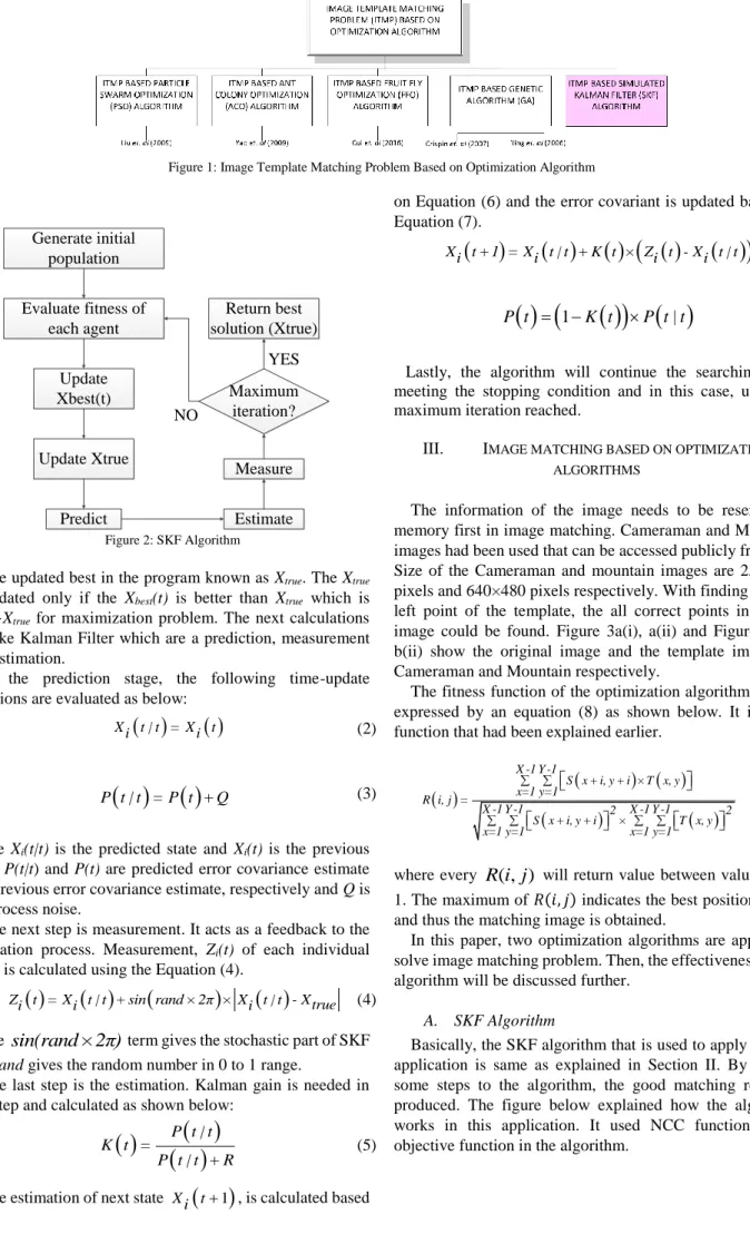
Optimization is a process to produce the best result with the least production process. In addition, with the process, the lost and error occurred can be reduced. Based on Figure 1, there are already a few of optimization algorithms used to solve this problem in the literature which are Particle Swarm Optimization (PSO) [2], Ant Colony Optimization (ACO) [4], Fruit Fly Optimization (FFO) [3] and Genetic Algorithm (GA) [5]. Every algorithm has their own ability to solve the matching problem. Those algorithms were proposed to solve image processing still lack in clarifying the real-time application problem. Reduction in computational time for the algorithm to solve the problem will make the algorithm more efficient. In the SKF algorithm, very few parameters needed
to be manipulated compared to GA. As reported in [3], FFO algorithm has some defects in the optimization process which is in the osphresis process. The individuals search in the osphresis phase for food by giving a random fly direction and distance, which is blind and reduces the search efficiency. Other than that, GA needs many steps such as crossover and mutation. These operators will increase the computational time of the system [2]. This paper uses SKF algorithm to solve the problem because there is no reported in literature use SKF in solving the image template matching problem. In other application, [6] is reported that SKF showed the better performance of the different application compared to PSO and Gravitational Search Algorithm (GSA).
The remainder of the paper mainly consists of the following work. The next section is the introduction of Simulated Kalman Filter (SKF) algorithm. How the two optimization algorithms solve the image matching problem has been further discussed in Section III. Next is section IV presented the experimental result and performance analysis of the algorithm. The conclusion and future work part are contained in the last section.
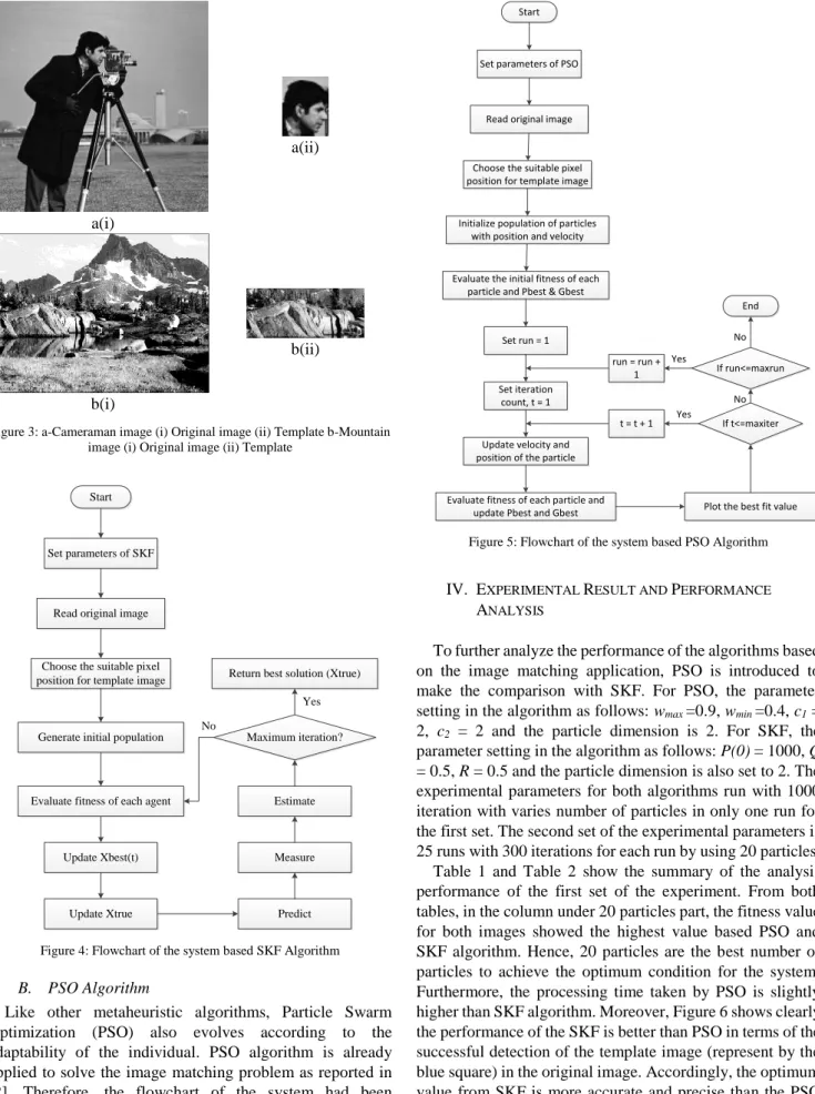
II. SIMULATED KALMAN FILTER (SKF) ALGORITHM Simulated Kalman Filter (SKF) was presented by Ibrahim et. al [7], [8] in 2015. SKF is a population-based metaheuristic algorithm introduced for continuous optimization problem and it is inspired by the estimation capability of Kalman Filter. The SKF algorithm is shown in Figure 2.
The algorithm is started with the generated initialization of the particles within the search space randomly. In addition, the initial value of error covariance estimate, P(0) the process noise value, Q and measurement noise value, R are needed during the initialization stage, which is also needed in Kalman Filter process.
After that, the fitness value of each particle needs to be calculated and the best fitness value of each iteration is recorded as Xbest(t). Image matching is considered as a maximization problem, therefore Equation (1) is used in this case.
Figure 1: Image Template Matching Problem Based on Optimization Algorithm Generate initial population Evaluate fitness of each agent Update Xbest(t) Predict Update Xtrue Measure Estimate Maximum iteration? Return best solution (Xtrue) YES NO Figure 2: SKF Algorithm
The updated best in the program known as Xtrue. The Xtrue is updated only if the Xbest(t) is better than Xtrue which is
Xbest>Xtrue for maximization problem. The next calculations are like Kalman Filter which are a prediction, measurement and estimation.
In the prediction stage, the following time-update equations are evaluated as below:
Xi t | t = Xi t (2)
P t | t = P t + Q (3)
where Xi(t|t) is the predicted state and Xi(t) is the previous state, P(t|t) and P(t) are predicted error covariance estimate and previous error covariance estimate, respectively and Q is the process noise.
The next step is measurement. It acts as a feedback to the estimation process. Measurement, Zi(t) of each individual agent is calculated using the Equation (4).
Zi t = Xi t | t + sin rand × 2π × Xi t | t - Xtrue (4) where
sin(rand×2π)
term gives the stochastic part of SKF and rand gives the random number in 0 to 1 range.The last step is the estimation. Kalman gain is needed in this step and calculated as shown below:
P t | t
K t =P t | t + R
(5)
The estimation of next state Xi
t1 , is calculated basedon Equation (6) and the error covariant is updated based on Equation (7).
Xi t +1 = Xi t | t + K t × Zi t - Xi t | t (6)
1
|P t K t P t t (7)
Lastly, the algorithm will continue the searching until meeting the stopping condition and in this case, until the maximum iteration reached.
III. IMAGE MATCHING BASED ON OPTIMIZATION
ALGORITHMS
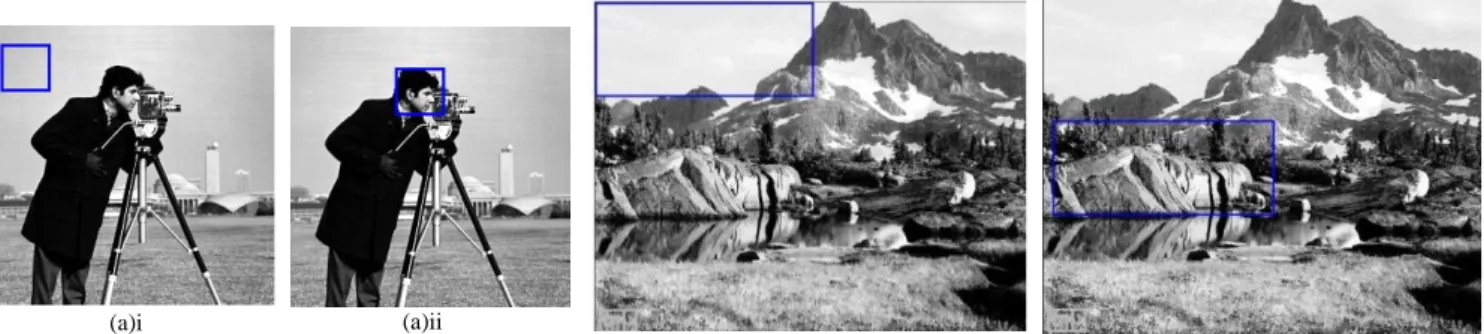
The information of the image needs to be reserved in memory first in image matching. Cameraman and Mountain images had been used that can be accessed publicly from [9]. Size of the Cameraman and mountain images are 256×256 pixels and 640×480 pixels respectively. With finding the up-left point of the template, the all correct points in source image could be found. Figure 3a(i), a(ii) and Figure 3b(i), b(ii) show the original image and the template image for Cameraman and Mountain respectively.
The fitness function of the optimization algorithm can be expressed by an equation (8) as shown below. It is NCC function that had been explained earlier.
X -1 Y -1 S x + i, y + i × T x, y x=1 y=1 R i, j = X -1 Y -1 2 X -1 Y -1 2 S x + i, y + i × T x, y x=1 y=1 x=1 y=1 (8)where every
R i j
( , )
will return value between value 0 and 1. The maximum of 𝑅(𝑖, 𝑗) indicates the best position for T, and thus the matching image is obtained.In this paper, two optimization algorithms are applied to solve image matching problem. Then, the effectiveness of the algorithm will be discussed further.
A. SKF Algorithm
Basically, the SKF algorithm that is used to apply for this application is same as explained in Section II. By adding some steps to the algorithm, the good matching result is produced. The figure below explained how the algorithm works in this application. It used NCC function as an objective function in the algorithm.
a(i)
a(ii)
b(i)
b(ii)
Figure 3: a-Cameraman image (i) Original image (ii) Template b-Mountain image (i) Original image (ii) Template
Start
Set parameters of SKF
Read original image
Choose the suitable pixel position for template image
Evaluate fitness of each agent Generate initial population
Update Xbest(t) Predict Update Xtrue Measure Estimate Maximum iteration? Return best solution (Xtrue)
No
Yes
Figure 4: Flowchart of the system based SKF Algorithm
B. PSO Algorithm
Like other metaheuristic algorithms, Particle Swarm Optimization (PSO) also evolves according to the adaptability of the individual. PSO algorithm is already applied to solve the image matching problem as reported in [2]. Therefore, the flowchart of the system had been summarized in Figure 5. There is some modification from the traditional PSO. It is by adding a few steps to make the algorithm suitable for this application. It also uses NCC function as the fitness function in the algorithm.
Start
Set parameters of PSO
Initialize population of particles with position and velocity
Evaluate the initial fitness of each particle and Pbest & Gbest
Set iteration count, t = 1
Evaluate fitness of each particle and update Pbest and Gbest
If t<=maxiter t = t + 1
Set run = 1
If run<=maxrun Read original image
Choose the suitable pixel position for template image
run = run + 1
End
Update velocity and position of the particle
Plot the best fit value No Yes
Yes No
Figure 5: Flowchart of the system based PSO Algorithm
IV. EXPERIMENTAL RESULT AND PERFORMANCE ANALYSIS
To further analyze the performance of the algorithms based on the image matching application, PSO is introduced to make the comparison with SKF. For PSO, the parameter setting in the algorithm as follows: wmax =0.9, wmin=0.4, c1 = 2, c2 = 2 and the particle dimension is 2. For SKF, the parameter setting in the algorithm as follows: P(0) = 1000, Q = 0.5, R = 0.5 and the particle dimension is also set to 2. The experimental parameters for both algorithms run with 1000 iteration with varies number of particles in only one run for the first set. The second set of the experimental parameters is 25 runs with 300 iterations for each run by using 20 particles. Table 1 and Table 2 show the summary of the analysis performance of the first set of the experiment. From both tables, in the column under 20 particles part, the fitness value for both images showed the highest value based PSO and SKF algorithm. Hence, 20 particles are the best number of particles to achieve the optimum condition for the system. Furthermore, the processing time taken by PSO is slightly higher than SKF algorithm. Moreover, Figure 6 shows clearly the performance of the SKF is better than PSO in terms of the successful detection of the template image (represent by the blue square) in the original image. Accordingly, the optimum value from SKF is more accurate and precise than the PSO algorithm according to the successful of matching attempt.
In addition, for the second set of the experiment, 25 runs had been tested independently to proof which algorithm is better and has a consistent result. Figure 7 had summarized the result of the image matching for both images. From the chart, it is clearly seen that percentage of successful detection
of SKF is higher than PSO for both images. Although, there is also a successful attempt made by PSO algorithm but not as often as SKF.
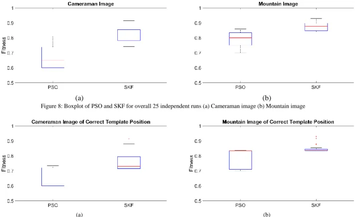
Boxplot was used to illustrate the quality and consistency of the algorithm. As for image matching problem is maximization problem, higher boxplot showed the better accuracy. In addition, the size of the boxplot represents to the
variance value that is, the small size of boxplot gives a better consistency. Figure 8 and Figure 9 show the boxplot of PSO and SKF for overall 25 independent runs and for correct template position respectively. Generally, from both figures, the performance of SKF is better than PSO. In order that, SKF is more accurate and precise algorithm for solve image matching problem.
(a)i (a)ii
(b)i (b)ii
Figure 6: (a) Cameraman image i PSO ii SKF (b) Mountain image I PSO ii SKF
Figure 7 Performance between PSO and SKF Algorithms Table 1
Summary of the PSO and SKF Algorithms Performance for Cameraman image
Image Cameraman
No of iteration 1000
No. of run 1
No. of particles 10 20 30 40
Algorithm PSO SKF PSO SKF PSO SKF PSO SKF
Fitness value 0.7126 0.7127 0.7126 0.7909 0.7126 0.7231 0.7353 0.7231 Processing time (seconds) 69.54 46.13 56.85 45.38 49.93 47.33 51.00 47.03
Table 2
Summary of the PSO and SKF Algorithms Performance for Mountain image
Image Mountain
No of iteration 1000
No. of run 1
No. of particles 10 20 30 40
Algorithm PSO SKF PSO SKF PSO SKF PSO SKF
Fitness value 0.8357 0.8361 0.8354 0.8541 0.8357 0.8357 0.8357 0.8357 Processing time (seconds) 105.11 83.07 127.76 108.12 148.32 133.17 196.35 153.65
12 4 36 32 0 10 20 30 40 Cameraman Mountain Perc en ta ge o f Su cce ss fu l De tection Images
Performance between PSO and SKF Algorithms
(a) (b)
Figure 8: Boxplot of PSO and SKF for overall 25 independent runs (a) Cameraman image (b) Mountain image
(a) (b)
Figure 9: Boxplot of PSO and SKF for Correct Template Position (a) Cameraman image (b) Mountain image.
V. CONCLUSION
This paper puts SKF algorithm into use in image matching problems and achieves satisfying effects. The percentage of matching result for Cameraman and Mountain are 36% and 32% accordingly which is higher than PSO algorithm. As for improved the SKF algorithm to solve the image matching problem, the parameters setting like P(0), Q and R of the system should be changed to achieve the better performance. In addition, the computational time is decreased greatly. The proposed algorithm can be applied to low and medium dimensional image to solve the image template matching problem and will apply to the high dimensional image later. However, the proposed algorithm is more accurate proven by the performance analysis showed in the other section.
For the future works will focus on to do image matching for more complex image and image matching for real-time application. Lastly, the important part of the system is to increase the percentage of successful image matching by adding image preprocessing techniques to the original image.
ACKNOWLEDGMENT
The work presented in the paper has been supported by Ministry of Higher Education under Fundamental Research Grant Scheme (FRGS) RDU 160105 and Universiti Malaysia Pahang Research Grant RDU 170378.
REFERENCES
[1] J. Zhang and G. Wang, “Image Matching Using a Bat Algorithm with Mutation,” vol. 203, pp. 88–93, 2012.
[2] X. Liu, W. Jiang, and J. Xie, “An Image Template Matching Method Using Particle Swarm Optimization,” 2009 Second Asia-Pacific Conf. Comput. Intell. Ind. Appl., pp. 83–86, 2009.
[3] W. Cui and Y. He, “Tournament Selection based Fruit Fly Optimization and Its Application in Template Matching,” no. 1, pp. 362–365.
[4] L. Yao, H. Duan, and S. Shao, “Adaptive Template Matching Based on Improved Ant Colony Optimization,” 2009 Int. Work. Intell. Syst. Appl., no. 1, pp. 1–4, 2009.
[5] A. J. Crispin and V. Rankov, “Automated inspection of PCB components using a genetic algorithm template-matching approach,”
Int. J. Adv. Manuf. Technol., vol. 35, no. 3–4, pp. 293–300, 2007. [6] K. Z. Mohd Azmi, Z. Ibrahim, and D. Pebrianti, “Simultaneous
computation of model order and parameter estimation for ARX model based on multi- swarm particle swarm optimization,” ARPN J. Eng. Appl. Sci., vol. 10, no. 22, pp. 17191–17196, 2015.
[7] Z. Ibrahim, N. Hidayati Abdul Aziz, N. Azlina Ab Aziz, S. Razali, M. Ibrahim Shapiai, A. Razak, S. Wahyudi Nawawi, and M. Saberi Mohamad, “A Kalman Filter Approach For Solving Unimodal Optimization Problems,” vol. 4, no. 5, 2010.
[8] Z. Ibrahim, N. H. A. Aziz, N. A. A. Aziz, S. Razali, and M. S. Mohamad, “Simulated Kalman Filter: A Novel Estimation-Based Metaheuristic Optimization Algorithm,” Adv. Sci. Lett., vol. 22, no. 10, pp. 2941–2946, Oct. 2016.
[9] “Image Matching « LTU – The Image Recognition API.” [Online]. Available: https://www.ltutech.com/technology/image-matching/. [Accessed: 29-Jul-2017].