Application of opposition-based learning concepts in reducing the power consumption in wireless access networks

Application of Opposition-Based Learning Concepts

in Reducing the Power Consumption

in Wireless Access Networks

Sotirios K. Goudos

Thessaloniki 54124, Greece Email: [email protected]

Margot Deruyck, David Plets, Luc Martens,

Wout Joseph

Department of Information Technology Ghent University

Ghent, Belgium

Email:{margot.deruyck, david.plets, luc.martens, wout.joseph}@intec.ugent.be

Abstract—The reduction of power consumption in wireless access networks is a challenging and important issue. In this paper, we apply Opposition-Based Learning (OBL) concepts for reducing the power consumption of LTE base stations. More specifically, we present a new Modified Biogeography Based Op-timization (BBO) algorithm enhanced with OBL techniques. We apply both the original BBO and the new Modified Opposition BBO (MOBBO) to network design cases to the city of Ghent, Belgium, with 75 possible LTE base station locations. We optimize the network towards two objectives: coverage maximization and power consumption minimization. Preliminary results indicate the advantages and applicability of our approach.

I. INTRODUCTION

Wireless access networks are currently large power con-sumers within ICT. In five years time (from 2007 till 2012), this power consumption has increased yearly with 10% [1]. It is expected that this amount will even increase in the next few years, as these networks need to expand in order to deal with the extreme growth of mobile devices and the higher bit rate demands required by these mobile devices. For the development of future wireless access networks, power consumption will become a key parameter [2]–[5]. A specified area, the target area, needs to be covered with a certain wireless technology. In this paper we consider Long Term Evolution (LTE) with a minimal power consumption. By selecting the most appropriate base station locations from a set of existing locations (from operators active in the target area) and tuning base station parameters such as the antennas input power, an energy-efficient network is obtained. Additionally, we optimize the network by taking into account Multiple Input Multiple Output (MIMO) for each base station and assuming that each base station could be either a macrocell or a femto-cell. Evolutionary algorithms (EAs) are suitable optimization techniques for solving the above-described problem.

Biogeography-based optimization (BBO) [6] is an evolu-tionary algorithm based on mathematical models that de-scribe how species migrate from one island to another, how new species arise, and how species become extinct. The way the problem solution is found is analogous to natures

way of distributing species. In [7] a new BBO algorithm based on opposition-based learning (OBL) called Oppositional Biogeography-Based Optimization (OBBO) was introduced. The basic idea of the OBL concept is to calculate the fitness not only of the current individual but also to calculate the fitness of the opposite individual. The benefits of using such a technique are that convergence speed may be faster and that a better approximation of the global optimum can be found. OBL techniques were also applied successfully to Differential Evolution in [8]. In all the above papers, OBL was applied to continuous domain problems. In [9] the OBBO concept was applied to specific discrete domain problems like the traveling salesman (TSP) and the vertex coloring problem. However, in the above paper the definition of the opposite point was problem-dependent.

In this paper we propose a new Modified Opposition BBO (MOBBO) that can be applied to the network design problems and to other discrete domain problems as well. The basic con-cept of the proposed algorithm is to decide using a predefined opposition probability if each decision variable in every D-dimensional individual is replaced by its opposite or not.

We apply MOBBO to three design cases for power reduction and coverage maximization for LTE networks. We compare results with the original BBO. Numerical results show that MOBBO outperforms the original BBO algorithm in terms of solution accuracy and convergence speed. This paper is organized as follows. We describe the problem formulation in Section II. The details of the MOBBO algorithm are given in Section III. In Section IV we present the numerical results. Finally, the conclusion is given in Section V.

II. FORMULATION

We address network planning optimization for LTE base stations. The concept and algorithms are used to perform network planning of 75 LTE base station locations in the city of Ghent, Belgium. This area covers about 6.85 km2_. The network optimization problem is to find the least possible number of base stations that operate with such input power

so that the coverage area is maximized. Therefore, there are two requirements; to minimize power consumption and to maximize coverage. The power consumption objective can be expressed as [2]: fpow(¯x) = 100 1−Pc(¯x) Pmax (1) where x¯ is the vector of a given solution, Pc(¯x) is the

calculated power consumption in Watts of the solution, and

Pmax is the maximum power consumption assuming that all base stations are active and operate at maximum input power. In case of a femtocell base station we consider a fixed power consumption of 12W. The details of the power consumption formulation can be found in [2]. The second objective is to cover the maximum possible percentage of the given area. The coverage functionfcov(¯x) specified by:

fcov(¯x) = 100

AtargetTA(¯x)

Atarget

(2) where Atarget is the area of the target area to be covered (in km2), and A(¯x) is the area covered by a given solution (in km2). In order to calculate the A(¯x) we first needed to calculate for each active base station the maximum allowable path loss, P Lmax (in dB). For this case, the link budget parameters for the LTE network of Table I are taken into account. The maximum rangeR (in meters) covered by each base station can be computed as in [2]. The area covered by a given solution is the union of all base stations coverage areas that are determined by each maximum range R. The above objectives can be combined using the following objective function [2]: F(¯x) =−(fcov(¯x) +kfpow(¯x)) with k=    0 if fcov(¯x)<90 (fcov(¯x)−90)2 5 if 90≤fcov(¯x)≥95 5 otherwise (3)

where the minus sign is used for minimization. The mini-mum value (-600) is obtained when bothfcov(¯x)andfpow(¯x)

equal to 100. This kind of global fitness function is chosen because of the trade-off between coverage and power con-sumption.

In this paper, we assume that all femtocell base stations are placed outdoor. Additionally, we consider the Walfis-chIkegami propagation model for path loss calculations. The above-mentioned problem can be solved using an evolutionary algorithm. It is an integer-programming problem, for which several different solutions exist. In this paper, we will apply the BBO and the MOBBO algorithms.

III. MODIFIEDOPPOSITIONALBIOGEOGRAPHY-BASED

OPTIMIZATION

The mathematical models of Biogeography are based on the work of Robert MacArthur and Edward Wilson in the early 1960s. Using this model, it was possible to predict the number

TABLE I

LINKBUDGET PARAMETERS FOR THELTENETWORK

Parameter Macrocell BS Femtocell BS

Frequency 2.6 GHz 2.6 GHz

Maximum input power base station antenna

43 dBm 33 dBm

Antenna gain of base station

18 dBi 4 dBi

Antenna gain of re-ceiver

0 dBi 0 dBi

Feeder loss base sta-tion

2 dB 2 dB

Feeder loss receiver 0 dB 0 dB

Fade margin 10 dB 10 dB

Yearly availability 100.00% 100.00% Interference margin 2 dB 2 dB Noise figure of

re-ceiver 8 dB 8 dB Implementation loss of receiver 0 dB 0 dB MIMO 1x1 1x1 Receiver SNR 1/3 QPSK = -1.5 dB 1/3 QPSK = -1.5 dB 1/2 QPSK = 3 dB 1/2 QPSK = 3 dB 2/3 QPSK = 10.5 dB 2/3 QPSK = 10.5 dB 1/2 16-QAM = 14 dB 1/2 16-QAM = 14 dB 2/3 16-QAM = 19 dB 2/3 16-QAM = 19 dB 1/2 64-QAM = 23 dB 1/2 64-QAM = 23 dB 2/3 64-QAM = 29.4 dB 2/3 64-QAM = 29.4 dB Bandwidth 5 MHz 5 MHz

Soft handover gain receiver 0 dB 0 dB Building penetration loss 0 dB (only outdoor coverage considered) 0 dB (only outdoor coverage considered) Height mobile

sta-tion

1.5 m 1.5 m

of species in a habitat. The habitat is an area that is geograph-ically isolated from other habitats. The geographical areas that are well suited as residences for biological species are said to have a high habitat suitability index (HSI). Therefore, every habitat is characterized by theHSIwhich depends on factors like rainfall, diversity of vegetation, diversity of topographic features, land area, and temperature. Each of the features that characterize habitability is known as suitability index variables (SIV). The SIVs are independent variables while HSI is the dependent variable.

Therefore, a solution to a D-dimensional problem can be represented as a vector of SIV variables [SIV1, SIV2, ...SIVD], which is a habitat or island.

The value of HSI of a habitat is the value of the objective function that corresponds to that solution and it is found by

HSI =F(habitat) =F(SIV1, SIV2, ...SIVD) (4)

Habitats with a highHSI are good solutions of the objec-tive function, while poor solutions are those habitats with a lowHSI. The immigration and emigration rates are functions of the rank of the given candidate solution. The rank of the given candidate solution represents the number of species in

a habitat. These are given by µk=E k Smax , λk=I 1− k Smax (5) where I is the maximum possible immigration rate, E is the maximum possible emigration rate, k is the rank of the given candidate solution, andSmaxis the maximum number of species (e.g. population size). The rank of the given candidate solution or the number of species is obtained by sorting the solutions from most fit to least fit, according to theHSIvalue (e.g. fitness). BBO uses both mutation and migration operators. The application of these operators to each SIV in each solution is decided probabilistically.

A. Opposition Based Learning (OBL)

The basic concept of OBL was originally introduced by Tizhoosh in [10]. The basic idea of OBL is to calculate the fitness not only of the current individual but also to calculate the fitness of the opposite individual. Then the algorithm selects the individual with the lower (higher) fitness value. At first we give the definitions for the basic concepts of OBL [10]–[12].

Definition (Opposite Number) let x∈ [a, b] be any real number. The opposite number is defined by

xO=a+b−x (6)

Definition (Opposite Point). Similarly if we extend the above definition to D-dimensional space then let

P(x1, x2, ...xD) a point where x1, x2, ...xD ∈ < and

xj ∈ [aj, bj] ∀j ∈ {1,2, ...D}. The opposite point

PO(xO1, xO2, ...xOD)is defined by its components

xOj=aj+bj−xj (7)

Definition (Semi-opposite Point) [13]. If we change the components of a point by its opposites only in some components and the other remain unchanged then the new point is a semi-opposite point. This is defined by

PSO(xSO1, xSO2, ..xSOj.., xSOD)

where∀j∈ {1,2, .., D}xSOj={xj or xOj (8)

For example in a two-dimensional space where each dimen-sion can be either 0 or 1 we consider the pointP1(0,1). Then the two semi-opposite points areP2(0,0)andP3(1,1), while the opposite point isP4(1,0).

B. Proposed Algorithm

In this paper we propose a OBBO version based on semi-opposite points. We call this algorithm Modified OBBO (MOBBO). We define a new control parameter named op-position probability po ∈ [0,1]. This parameter controls if

a SIV variable in a habitat will be replaced by its opposite or not. Moreover as in previous opposition-based algorithms [7]–[9] we use the jumping rate parameter jr ∈[0,1] which

controls in each generation if the opposite population is created or not. The opposite based algorithms require two additional

parts to the original algorithm code; the opposition-based population initialization and the opposition-based generation jumping [7]–[9]. The opposition based population initialization for MOBBO is described below. For this caselowj,upperjare

the lower and upper limits in the j-th dimension respectively.

Algorithm 1 Opposition-Based Population Initialization

1: Generate uniform distributed random populationP 2: fori=1 toN P do

3: Generate semi-opposite populationOPs

4: forj=1 toD do

5: if rnd[0,1]< po then

6: xosi,j =lowj+upperj−xi,j

7: else

8: xosi,j =xi,j

9: end if

10: end for

11: end for

12: Initial population= the fittest amongP andOPs

The opposition-based generation jumping follows a similar approach. The algorithm description is given below. Theminj,

maxj are the minimum and maximum values of the j-th

dimension in the current population respectively.

Algorithm 2 Opposition-Based Generation Jumping

1: ifrnd[0,1]< jr then

2: fori=1 toN P do

3: Generate semi-opposite populationOPs

4: forj=1 toD do

5: if rnd[0,1]< po then

6: xosi,j = minj+ maxj−xi,j

7: else 8: xosi,j =xi,j 9: end if 10: end for 11: end for 12: end if

13: Select fittest among current population P andOPs

Therefore, the MOBBO algorithm can be described as follows:

1) Initialize the MOBBO control parameters.

2) Initialize a random population of N P habitats (phase vectors) from a uniform distribution. Set the number of gen-erations Gto one.

3) Initialize the opposite population according to algorithm 1.

4) Map the HSI value to the number of species S, the immigration rate λk, the emigration rateµk for each solution

(phase vector) of the population.

5) Apply the migration operator for each non-elite habitat based on immigration and emigration rates using (5).

6) Apply the mutation operator. 7) Evaluate objective function value.

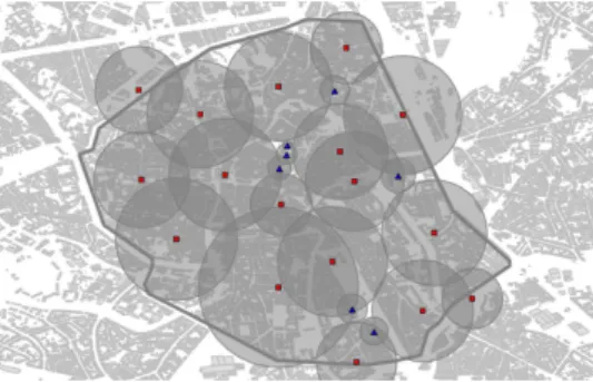
Fig. 1. Map of the city of Ghent with the active LTE base stations for the first case. The circles represent the coverage area of each base station.

8) If rnd[0,1] < jr calculate the opposite population

according to algorithm 2.

9) Repeat step 4 until the maximum number of generations

Gmax or the maximum number of objective function evalua-tions is reached.

IV. NUMERICALRESULTS

We consider 75 possible LTE base stations. Each one can be active (1) or not (0). If the base station is active then the range of the input power of the base station antenna is from 0 to 43 dBm, and 0 to 33dBm with a step of 1dBm for macrocell and femtocell base stations respectively. We compare MOBBO with the original BBO algorithm. Both algorithms are executed 20 times. The results are compared. The population size is set to 100 and the maximum number of generations is set to 1000 iterations. The maximum number of objective function evaluations is set to 100000. The first case is that of an LTE network with macrocell base stations without Multiple Input Multiple Output (MIMO). The total number of decision variables is 2x75 for this case (each base station can be active or not and have a value of input power).The best-obtained result for MOBBO is that of a network with about 95% coverage and 24.5% power consumption (which means that the power consumption is 24.5% of the maximum power consumption assuming that all base stations are active and operate at a maximum input power). The solution consists of 20 base stations. This solution is visualized in Fig. 1. Correspondingly, the best-obtained result for the original BBO is that with 95% coverage and 25.3% power consumption, which consists of 21 base stations.

The second case is that of an LTE network supporting both macrocell and femtocell base stations. In this case each base station could be either off (0), macrocell active (1), or femtocell active (2). MOBBO has produced a network that has 95% coverage and 24.4% power consumption. The number of base stations in this network is 23. Fig. 2 visualizes this case. The best result with BBO is that of a network consisting of 21 base stations with 95% coverage and 24.7% power consumption. Both results are very similar in this case.

The final example is that of an LTE network supporting both macrocell and femtocell base stations with MIMO. Thus, each base station has a different number of transmitting and

Fig. 2. Map of the city of Ghent with the active LTE base stations for the second case. The circles represent the coverage area of each base station. The red squares indicate the macrocell base stations while the blue triangles indicate the femtocell base stations.

TABLE II

BEST-OBTAINED RESULTS COMPARISON. THE SMALLER VALUES ARE IN BOLD.

Algorithm Best objective function value Case 1 Case 2 Case 3 BBO -468.64 -471.62 -548.97 MOBBO -472.65 -473.12 -550.52

receiving antennas. Each base station could consist of Nt

transmission and Nr reception antennas. The possible values

for Nt and Nr is 1, 2, or 4. Therefore, the total number of

unknowns increases to 4x75. The best-obtained result for this case using MOBBO is a network with 95% coverage and 8.9% power consumption. This solution requires 24 LTE base stations. The network is shown in Fig.3. BBO has obtained a best solution with 21 bases stations with 95% coverage and 9.2% power consumption. The best obtained objective function values for each case are shown in Table II. It is obvious that MOBBO has outperformed the original BBO algorithm. Table III reports the average fitness values for different numbers of objective-function evaluations. Again MOBBO outperforms BBO which shows faster convergence.

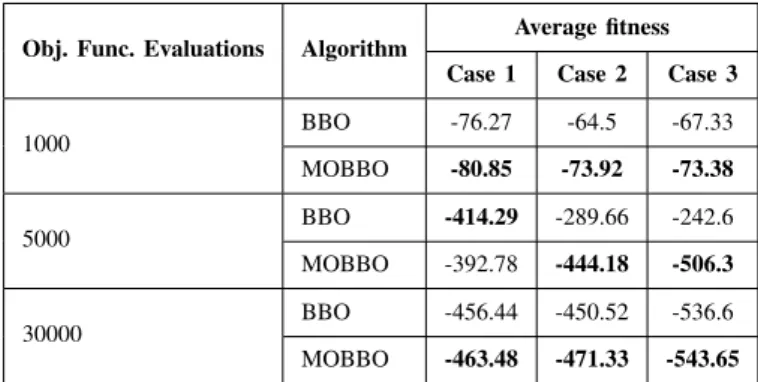
TABLE III

AVERAGE FITNESS COMPARISON. THE SMALLER VALUES ARE IN BOLD.

Obj. Func. Evaluations Algorithm Average fitness Case 1 Case 2 Case 3

1000 BBO -76.27 -64.5 -67.33 MOBBO -80.85 -73.92 -73.38 5000 BBO -414.29 -289.66 -242.6 MOBBO -392.78 -444.18 -506.3 30000 BBO -456.44 -450.52 -536.6 MOBBO -463.48 -471.33 -543.65 V. CONCLUSION

In this paper, we have addressed the problem of designing LTE networks for optimal coverage with the lowest power

con-Fig. 3. Map of the city of Ghent with the active LTE base stations for the third case supporting MIMO. The circles represent the coverage area of each base station. The red squares indicate the macrocell base stations while the blue triangles indicate the femtocell base stations.

sumption. We have proposed a novel design approach based on a new Oppositional-based BBO algorithm. The proposed algorithm outperformed the original BBO algorithm in terms of solution accuracy and convergence speed. The numerical results that we have shown have proven the effectiveness of this approach. In our future work, we will study further the capabilities of this new algorithm.

REFERENCES

[1] W. Van Heddeghem, S. Lambert, B. Lannoo, D. Colle, M. Pickavet, and P. Demeester, “Trends in worldwide ict electricity consumption from 2007 to 2012,”Computer Communications, vol. 50, pp. 64–76, 2014. [2] M. Deruyck, E. Tanghe, W. Joseph, and L. Martens, “Modelling and

optimization of power consumption in wireless access networks,” Com-puter Communications, vol. 34, no. 17, pp. 2036–2046, 2011. [3] M. Deruyck, W. Vereecken, W. Joseph, B. Lannoo, M. Pickavet, and

L. Martens, “Reducing the power consumption in wireless access net-works: Overview and recommendations,”Progress In Electromagnetics Research, vol. 132, pp. 255–274, 2012.

[4] M. Deruyck, W. Joseph, and L. Martens, “Power consumption model for macrocell and microcell base stations,”European Transactions on Telecommunications, vol. 25, no. 3, pp. 320–333, 2014.

[5] M. Deruyck, W. Joseph, E. Tanghe, and L. Martens, “Reducing the power consumption in lte-advanced wireless access networks by a capacity based deployment tool,”Radio Science, vol. 49, no. 9, pp. 777– 787, 2014.

[6] D. Simon, “Biogeography-based optimization,”IEEE Transactions on Evolutionary Computation, vol. 12, no. 6, pp. 702–713, 2008. [7] M. Ergezer, D. Simon, and D. Du, “Oppositional biogeography-based

optimization,” inConference Proceedings - IEEE International Confer-ence on Systems, Man and Cybernetics, 2009, pp. 1009–1014. [8] R. S. Rahnamayan, H. R. Tizhoosh, and M. M. A. Salama,

“Opposition-based differential evolution,”IEEE Transactions on Evolutionary Com-putation, vol. 12, no. 1, pp. 64–79, 2008.

[9] M. Ergezer and D. Simon, “Oppositional biogeography-based optimiza-tion for combinatorial problems,” in2011 IEEE Congress of Evolution-ary Computation, CEC 2011, 2011, pp. 1496–1503.

[10] H. R. Tizhoosh, “Opposition-based learning: A new scheme for machine intelligence,” inProceedings - International Conference on Computa-tional Intelligence for Modelling, Control and Automation, CIMCA 2005 and International Conference on Intelligent Agents, Web Technologies and Internet, vol. 1, 2005, pp. 695–701.

[11] ——, “Reinforcement learning based on actions and opposite actions,”

Proceedings of the ICGST International Conference on Artificial Intel-ligence and Machine Learning, pp. 94–98, 2005.

[12] H. R. Tizhoosh and M. Ventresca, Oppositional Concepts in Com-putational Intelligence, ser. Oppositional Concepts in Computational Intelligence. New York: Springer, 2008.

[13] F. Mohseni Pour and A. A. Gharaveisi, “Opposition-based discrete action reinforcement learning automata algorithm case study: Optimal design of a pid controller,” Turkish Journal of Electrical Engineering and Computer Sciences, vol. 21, no. 6, pp. 1603–1614, 2013.