NUMERICAL HYDRO- MORPHODINAMIC 2DH MODEL FOR THE SHALLOW WATERS

(1)

(2)

Università Politecnica delle Marche

Dipartimento di Idraulica, Strade, Ambiente e Chimica

Scuola di Dottorato di Ricerca in Scienze dell’Ingegneria Curriculum in Ingegneria dei Materiali, delle Acque e dei Terreni ---

NUMERICAL

HYDRO-MORPHODINAMIC 2DH MODEL

FOR THE SHALLOW WATERS

Ph.D. Dissertation of:

Matteo Postacchini

Advisor:

Prof. Ing. Alessandro Mancinelli

Co-Advisor:

Prof. Maurizio Brocchini

Supervisor of the Ph.D. School: Prof. Graziano Cerri

(3)

(4)

Scuola di Dottorato di Ricerca in Scienze dell’Ingegneria Curriculum in Ingegneria dei Materiali, delle Acque e dei Terreni ---

NUMERICAL

HYDRO-MORPHODINAMIC 2DH MODEL

FOR THE SHALLOW WATERS

Ph.D. Dissertation of:

Matteo Postacchini

Advisor:

Prof. Ing. Alessandro Mancinelli

Co-Advisor:

Prof. Maurizio Brocchini

Supervisor of the Ph.D. School: Prof. Graziano Cerri

(5)

(6)

(7)

(8)

Acknowledgements

I wish to thank all the research team of the Dipartimento di Idraulica, Strade, Ambiente e Chimica – Sezione Idraulica for the support during the entire three-years period of PhD. In particular, I would like to thank Prof.Ing. Mancinelli and Prof. Brocchini for the essential contribution in the development of this work, for both numerical and experimental part. Then I would like to thank, for their precious and helpful aid, Marc Landon and Camille Chauvigné, who contributed to the development of the numerical hydro-morphodynamic solver, and Dott.Ing. Lorenzoni, who worked with me at the experiments performed in the wave flume of the Hydraulic Laboratory of the Università Politecnica delle Marche of Ancona.

Finally, thank to Prof. Fraccarollo for the useful data provided for the validation tests of the numerical solver.

(9)

(10)

Abstract

In the present thesis a hydro-morphodynamic numerical model is illustrated as a novel contribution to the investigation and prediction of nearshore flows and seabed changes forced by waves and currents. The model includes a robust hydrodynamic solver for the integration of the Nonlinear Shallow Water Equations (NSWE) and a rather flexible solver for the resolution of the Exner equation (used to evaluate the morphological evolution of the sea bottom). Coupling of NSWE and Exner equation and updating of the solution is made by means of a sequential splitting scheme.

The model has been validated by reproducing both numerical/analytical tests, present in the literature of the last years, and laboratory experiences, performed in the Hydraulic Laboratory of the Università Politecnica delle Marche (AN). The simulation of the existent theoretical solutions led to consistent results for what concerns both hydrodynamics and morphodynamics, especially in the prediction of the seabed evolution due to either bed-load or suspended-load transport after dam-break and swash events.

The comparison between numerical results of the solver and experimental data is partially exhaustive. In fact, the solver reproduces fairly well the main bottom features in the presence of spectral waves but fails when regular waves are forced, because of “laboratory effects” occurred in the wave flume.

(11)

List of Figures

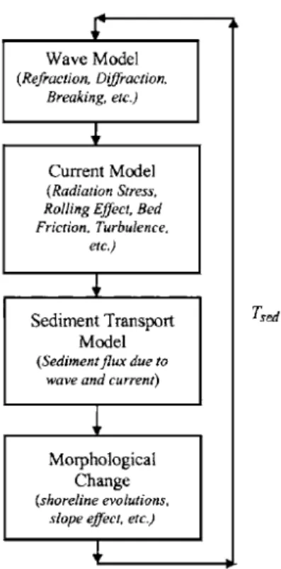
Figure 1 Sequential computation in CAM models (adapted from Ding et al., 2006).

Figure 2 Vertical flow structure; from the top to the bottom: pure-water layer, flowing mixture of water and grains, granular substratum. Γw, Γsand Γbare the interfaces between

air and water, water and mixture, mixture and bed, respectively (adapted from Fraccarollo & Capart, 2002).

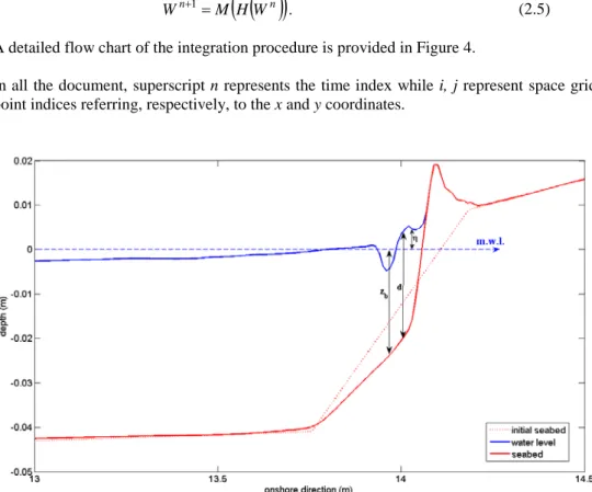
Figure 3 Sketch of seabed profile and free surface elevation. Figure 4 Flow chart of the computational schemes.

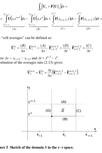
Figure 5 Sketch of the domain S in the x−t space.

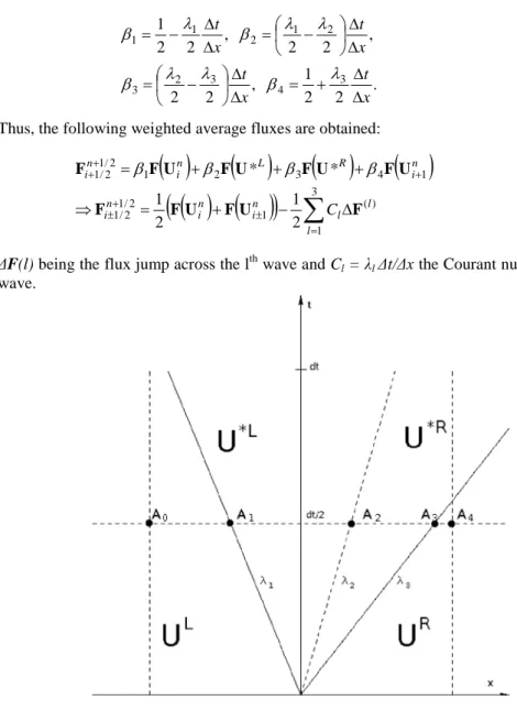
Figure 6 Flux computation from one specific Riemann problem in the x−t space.

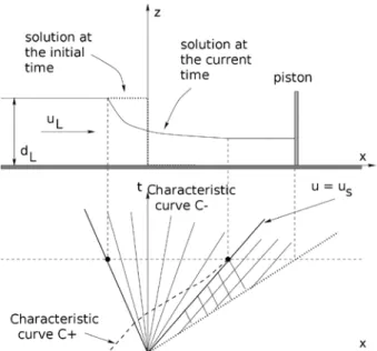
Figure 7 Sketch of the solution of the shoreline Riemann problem and analogy with the moving piston.

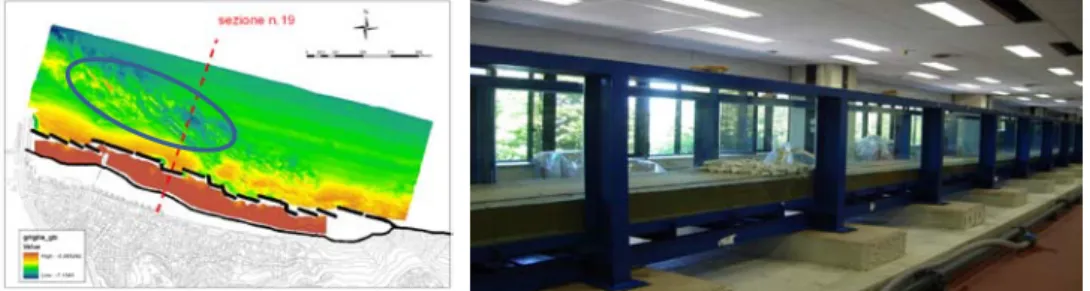
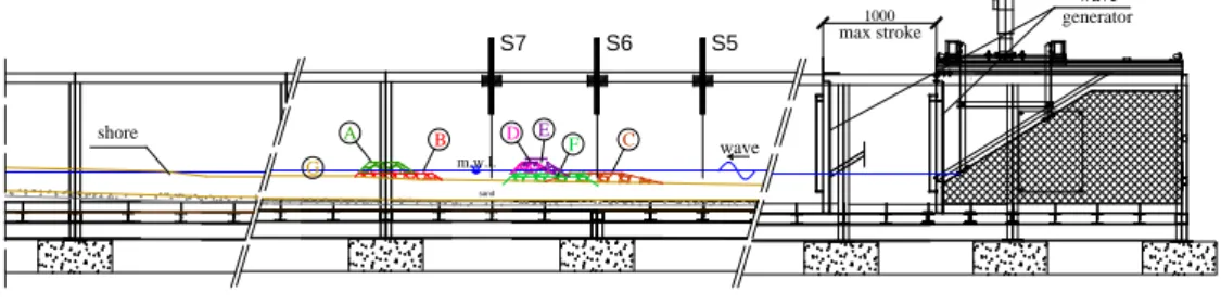
Figure 8 Bathymetric map (left) and reproduced movable-bed model in the flume (right). Figure 9 Sketch of the flume: shoreline (left), breakwaters at the tested positions (middle) and wave generator (right); S5, S6 and S7 give the positions of three wave gauges.

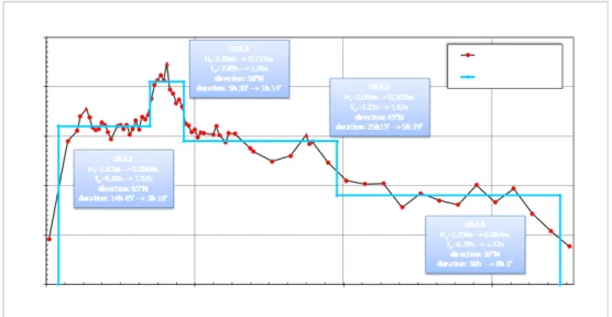
Figure 10 Chronological evolution of the sea-storm OS1 with wave characteristics (Hs, Tp, direction and duration) of each phase, at both prototype and model conditions.

Figure 11 Superposition of the bed profiles after each phase of the sea storm OS3 (September 2004) for configuration D.

Figure 12. Comparison among the final profiles due to OS2 for emerged configurations A and D (green and magenta line, top panel) and for submerged configurations B and C (red and yellow line, bottom panel); the black dotted line represents the initial profile; horizontal and vertical scales are in millimeters.

Figure 13 Snapshots from the experimental tests of Taipei, at t = 0s, 0.1s, 0.2s, 0.3s, 0.4s, 0.5s (left panels, from the top to the bottom), and Louvain, at t = 0.25s, 0.50s, 0.75s, 1.00s (right panels, from the top to the bottom, adapted from FC02).

Figure 14 Results from Taipei tests after t = 0.5s : black lines give the experimental results, green lines the results by FC02, red lines numerical solutions of the HM solver; solid lines refer to the still water level Γw, dash-dotted lines to the Γs limit, dashed lines to the bottom

level Γb.

Figure 15 Results from Louvain tests after t = 1s : black lines give the experimental results, green lines the results by FC02, red lines numerical solutions of the HM solver; solid lines

(16)

refer to the still water level Γw, dash-dotted lines to the Γs limit, dashed lines to the bottom

level Γb.

Figure 16 Numerical results of KE09’s model (in red) and of the HM solver (in blue), at time t = 5s after a dam-break event; from top to bottom: dimensionless depth, velocity and bottom location for q = Au3, where A = 1×10−3 s2m−1.

Figure 19 Numerical results of KE09’s model (in red) and of the HM solver (in blue), at time t = 5s after a dam-break event; from top to bottom: dimensionless depth, velocity and bottom location for q = Adu3, where A = 1.5×10−2 s2m−2.

Figure 20 Numerical results of KE09’s model (in red) and of the HM solver (in blue), at time t = 5s after a dam-break event; from top to bottom: dimensionless depth, velocity and bottom location for q = Adu3, where A = 4×10−3 s2m−2.

Figure 21 PH05 solution for the net fluxes Q~ (panel a) and the instantaneous flux q~ (panel b): (a) dashed lines give the net fluxes occurring during the uprush (positive values) and the backwash (negative values), the solid line gives the net flux over a cycle; (b) solid lines give the flux at sampling points located at x~ = 0.25, 0.5, 0.75, 1 (adapted from PH05).

Figure 22 Spatial evolution of Q~ (panels a, c, e) and temporal evolution of q~ (panels b, d,

f) from the HM solver, obtained by using a friction coefficient C_τ = 0.002 (top panels), C_τ = 0.005 (middle panels) and Cτ = 0.01 (bottom panels).

Figure 23 HM-solver results: cross-section seabed evolution in the absence of structures (configuration G) under the irregular wave forcing OS11.

Figure 24 HM-solver results: cross-section seabed evolution in the absence of structures (configuration G) under the regular wave forcing OR.

Figure 25 HM-solver results: cross-section seabed evolution in the presence of a submerged structure (configuration B) under the irregular wave forcing OS11.

Figure 26 HM-solver results: cross-section seabed evolution in the presence of a submerged structure (configuration B) under the regular wave forcing OR.

Figure 27 Seabed evolution for configuration G under the regular wave forcing OS11: comparison of the final results of the HM solver (solid red line) and flume experiments (solid green line); initial seabed (dotted red line) and water level at the final numerical output (in blue) are also shown.

Figure 28 Seabed evolution for configuration G under the regular wave forcing OR: comparison of the final results of the HM solver (solid red line) and flume experiments

(17)

(solid green line); initial seabed (dotted red line) and water level at the final numerical output (in blue) are also shown.

Figure 29 Seabed evolution for configuration B under the irregular wave forcing OS11: comparison of final results coming from HM solver (solid red line) and flume experiments (solid green line); initial seabed (dotted red line) and water level at the final numerical output (in blue) are also shown.

Figure 30 Seabed evolution for configuration B under the regular wave forcing OR: comparison of final results coming from HM solver (solid red line) and flume experiments (solid green line); initial seabed (dotted red line) and water level at the final numerical output (in blue) are also shown.

Figure 31 Sketch of the flows interesting the piling-up phenomenon in the presence of emerged (top figure) or submerged (bottom figure) breakwaters.

Figure 32 Representative sketch of the three-layer distribution: sea level, moving seabed and rigid seabed.

(18)

(19)

List of Tables

Table 1 Main geometrical characteristics of the tested breakwaters, at model scale. Table 2 Characteristics of the reproduced waves at model scale.

(20)

Chapter 1. Introduction

1.1. Wave dynamics in the nearshore zone

The marine region that is the closest to the emerged beach is called “nearshore zone”. Its dynamics is dominated by many parameters that are involved in several physical processes, concerning both hydrodynamics and morphodynamics. The main forcing of all these processes are waves and the induced currents that generate significant velocity fields, acting directly on the sea bottom and providing important morphological changes. In particular, surface gravity waves propagating across the continental shelf to the beach, wave-induced currents in the surf zone, longshore and cross-shore sediment motions are the phenomena that induce most of the beach evolution.

Knowledge of all these processes is fundamental for beach erosion prediction, nourishment management, maintenance and dredging of navigation channels and designing of shore protection structures. The forecast of the beach evolution, for what concerns accretion/evolution processes, is, nowadays, one of the main topics and targets of coastal research.

As described by Hamm et al. (1993) the wave propagation from the offshore to the coast induces large hydrodynamic and morphodynamic changes, especially when the water depth is not large and interferences with the seabed become important.

The seabed variation induces effects such as refraction, diffraction, shoaling and breaking. The latter is such a strong phenomenon that leads to wave reduction and seabed evolution in virtue of the energy transfers induced by such a dissipative phenomenon. In that portion of the nearshore region that is commonly called “surf zone” many processes connected with breaking take place: first an initial decay of the waves and a rapid change of their shape occurs because of wave breaking (in the “outer surf zone”); then a slow evolution of the waves and the achievement of a quasi-steady state similar to that of moving hydraulic jumps (within the “inner surf zone”); finally run-up and run-down events in correspondence of the “swash zone”.

All these processes, forced by the waves approaching the shore, induce strong increases of the velocity field, which, in turn, force significant sediment motions, especially in the swash zone, where the wave uprush and backwash lead to a relevant seabed evolution. At

(21)

the same time, bottom changes induce significant variations of the hydrodynamic conditions. In other words a feedback mechanism exists such that the hydrodynamics affect the morphodynamics and vice versa.

1.2. The modeling of the nearshore sediment transport

During the last decades many progresses have been made in the study of the nearshore morphodynamics, because several experiences have been carried out all over the world, both in the laboratories and directly in the field. Also many numerical and analytical models have been developed and upgraded in the years, on the basis of the physical and mathematical tools that are available for the correct representation of waves, currents and sediment transport.

The aim to give the best representation of the beach evolution, induced by the hydrodynamic field due to both waves and currents occurring in the nearshore zone, has been pursued with more incisiveness in the last decades and numerical simulations are becoming an indispensable tool to reach such a scope.

As an example, wave breaking is a very complex phenomenon, but it can be reproduced by means of hydrodynamic solvers that enable to simulate the breaker propagation through the surf zone and its evolution from the breaking line to the shore. However, the natural morphological processes and the mechanisms of sediment transport have not been fully understood neither described adequately by physical principles and mathematical analyses (Ding et al., 2006).

In order to simulate the morphological processes within reasonably short computational times, a series of constraints and approximations can be applied to the numerical solver. De Vriend et al. (1993) classified the numerical models for practical simulations of morphological processes into four types: 1) one-dimensional (1D) longshore coastline models; 2) two-dimensional (2DV) cross-shore coastal profile models; 3) two-dimensional-horizontal (2DH) morphological models; 4) fully three-dimensional (3D) local morphological models.

Solvers of the first group enable the users to study the evolution of both longshore sediment transport and shoreline. 2DV cross-shore models predict only the vertical variations of coastal profiles, but not the variations of the longshore sediment transport. 2DH models enable to reproduce all the phenomena occurring in the nearshore area, by means of an average of the vertical distributions of all the variables involved in both wave and current processes. The numerical solvers of class 4) of above are the most complete and, together with the 2DH models, they represent all the longshore and cross-shore morphological changes, but also take into account the vertical distributions of all the terms that are involved in these processes (i.e. velocity, sediment transport, etc).

However, fully-3D morphological models are, usually, used to predict the hydro-morphodynamic evolution of a relatively small field and over a short period. In fact,

(22)

because of their complexity, the computation time is large and they appear not suited to reproduce a long event acting in a large spatial domain.

In the recent period the evolution of morphodynamic solvers focused especially on the prediction of two-dimensional horizontal patterns that are related to the velocity field induced by water motions. Hence, 2DH depth-averaged models can well represent bed evolution in large-scale areas, even if also the quasi-3D models found a good success in the last decades. As an example, Zyserman & Johnson (2002) worked on a quasi-3D model where an empirical 3D shear stress distribution allows to take into account the three-dimensional effect of sediment transport, while Ding et al. (2006) developed a quasi-3D model (Q3DCAM) that is both robust as a 2DH model and able to include the effects of the vertical variations of currents due to the surface roller characterizing breaking waves. For what concerns the classical 2DH depth-averaged models for the nearshore zone, De Vriend (1987) claimed that they are typically characterized by two main modules, each providing a different computation in two separated steps. During the “fixed-bottom step” water and sediment motions are evaluated without providing any modification of the bed, that is taken as rigid. The “changing-bottom step” consists in the evaluation of the bottom variation, while the other variables are fixed. As a result, the strong approximation, due to the separated treatment of hydrodynamics and morphodynamics, does not induce a perfect representation of nature but, at the same time, computational times are small. In summary, it seems that what the approach chosen gives is the best compromise between appropriate numerical solutions and reduced computational costs.

As a consequence of this need, different types of numerical solvers based on separated modules rose in the last decades, with the aim to study separately all processes (waves, current, sediment transport) and to update them in a “compound morphological model” (De Vriend et al., 1993). The connections among all modules and the way to represent the processes leads to more or less complicated codes (“Initial Sedimentation/Erosion models”, “Medium-Term Morphodynamic models”, etc).

As an example of the numerical structure presented above, Coastal Area Morphological (CAM) models can be considered. In order to simulate at best the morphodynamic changes and the shoreline evolutions (Ding et al., 2006), a “process-based approach” is used in such models, i.e. wave field, current field and seabed changes are computed sequentially and not at the same time. The result is a new bathymetry, representing the bottom input for the next time step, as shown in Figure 1.

This procedure is the basis of a wave-current-morphological model and enables to simulate the long-term morphological processes by using an empirical sediment transport model, even if calibration/validation of such a model is required before applying it to a real-life coastal problem. In fact, it is necessary to check if the modeling of waves, currents and sediment transport evaluates correctly the main processes occurring during the wave propagation and if each module of the solver predicts with reasonable accuracy all the parameters of interest. Furthermore, it is important to have a code robust enough to simulate the long-term morphodynamic evolution by selecting a reasonably long feedback period Tsed (see Figure 1).

(23)

Figure 1 Sequential computation in CAM models (adapted from Ding et al., 2006).

1.2.1. The hydrodynamics equations

In the attempt to reproduce at best the whole hydrodynamics, two main approximations of the classical Navier-Stokes equations for the nearshore zone are used: the Nonlinear Shallow Water Equations (NSWE) and the Boussinesq-type equations.

In the last decades the fashionable Boussinesq-type models led to very interesting solutions in several coastal applications, though such a modeling was still limited because of some important problems. In fact, the treatment of phenomena like the shoreline motion, the wave breaking and the propagation of breaking fronts, were not adequate. Hence, many studies were dedicated to improve the mentioned limitations, and a more mature generation of Boussinesq-type models is currently available, which better represents breaking waves (e.g. see Brocchini et al., 1992) and frequency dispersion properties (e.g. see Madsen & Schäffer, 1998) to extend the models’ validity to the surf zone and to the deep waters, respectively.

NSWE models are very good for simulating both wave propagation over the “inner surf zone” and swash zone. Within such models, wave breaking is represented as a

(24)

discontinuity of the water flow. This approach gives, at the same time, a simple interpretation of a very complicated phenomenon and an incorrect location of the breaking point, which is always placed too far offshore than what found in experiments. Such a disadvantage is due to the absence of frequency dispersion so that the predicted hydrodynamics in the “outer surf zone” is not completely consistent with nature. However, applications of NSWE solvers to nearshore flows often lead to good results, because of the quasi-steady state of the shallow-water breakers.

1.2.2. The Exner equation

The morphodynamics can be fairly well described by means of the Exner equation, that represents the solid mass conservation law. Starting from the velocity field, such a conservation law enables to predict the seabed changes by means of the sediment transport variation over the horizontal plane. Usually, the nearshore sediment can be mobilized in three different modes (as described in Fredsøe, 1993): bed-load, sheet flow and suspended-load. They distinctly characterize different portions of the water column that is interested by the sediment motion. The first mode of transport refers to sediments that are in almost continuous contact with the bed and depends directly on the bed shear stress, that should be small enough for this mode to occur. Suspended sediments move through the whole water column and are forced by the water flows. The sheet flow is a specific transport mode that is can be described as being in between suspension and bed-load transport. It concerns sediments moving over the bed, without any contact, in a well-defined layer and occurs when shear stresses are rather large.

Generally, numerical models represent the sediment transport as the sum of only two contributions: bed-load and suspended-load transport, without taking into account the sheet flow motion. Many formulas have been developed in the recent years and discussions about them (e.g. Camenen & Larson, 2008) suggest the application field for each relation and also which ones are most suited to be implemented in a model.

In order to obtain both hydrodynamic and morphodynamic evolutions a weakly-coupled model, built on a finite-volume scheme, has been developed, based on various sediment transport formulations, for both bed-load and suspended-load.

1.3. The coupling issue

A large amount of studies concerning the morphodynamics in both surf and swash zone have led to the development of several mathematical models in the last years. They are characterized by different features and different complexities depending on the aim of the solver at hand. Several studies have been carried out to understand the behavior of the swash zone dynamics under either periodic or impulsive (dam-break type) wave forcing. In fact, because many variables are involved in the large amount of processes concerning the

(25)

swash motion (such as sediment transport, groundwater dynamics, beachface morphology, water-table contribution, etc, for more details see Masselink & Puleo, 2006), the swash zone represents one of the most difficult areas to be described of the entire nearshore. Because of the interaction among all the involved parameters, the correct reproduction of the swash zone morphological evolution is rather difficult and many models, both numerical and analytical, have been built to simulate such a dynamics as well as possible, by applying sediment transport formulas depending on one or both shallow-water hydrodynamic variables (depth and depth-averaged velocity).

In the attempt to provide a fairly good illustration of the state-of-the-art of mathematical modeling concerning the nearshore zone, in the following subsections a special attention is given to the description of some of the most recent works that are available in the literature. Decoupled and coupled, as well as analytical and numerical models are analyzed. It is important to note that the equations, used to describe the hydrodynamic processes occurring in the nearshore area, i.e. the NSWE, are shared by all the considered models.

1.3.1. A fully-coupled analytical/numerical model of bed-load transport: velocity-based law (Kelly & Dodd, 2010)

The work of Kelly & Dodd (2010) is based on the description of a mathematical model in which hydrodynamics and morphodynamics are directly coupled. The result is that seabed and flow evolution are integrated within the same time step and within the constraints imposed by the inviscid shallow-water dynamics and by a simple sediment transport relation. An uncoupled model has also been developed in order to understand the differences existing with the fully-coupled one.

Furthermore, the model does not take into account contributions of water infiltration/exfiltration, sediment storage, settling lag, advection of sediment from the surf zone and bed shear stress, which are fundamental processes occurring on the beachface during swash events (e.g. see Brocchini & Baldock, 2008).

The mathematical model predicts the seabed changes and the velocity fields as forced by a single swash event and enables a comparison with the analytical solution of Shen & Meyer (1963).

The flow field in the swash zone is well represented by the NSWE, that, in dimensional form, are written as:

0 = ∂ ∂ + ∂ ∂ + ∂ ∂ x u d x d u t d , (1.1)

(

)

0 = ∂ + ∂ + ∂ ∂ + ∂ ∂ x z d g x u u t u , (1.2)

where d(x, t) is the total water depth, u(x, t) the depth-averaged flow velocity along the horizontal x-direction, z(x, t) the beach surface level and g is gravity acceleration.

(26)

The sediment transport equilibrium is given by the continuity equation for the solid mass, i.e. by the following formulation of the Exner equation:

0 = ∂ ∂ + ∂ ∂ x q t z _ξ , (1.3)

where q is the horizontal sediment flux and

ξ

=

1 (

1 −

p

)

a coefficient dependent on the beach porosity p.

Generally, the sediment transport contribution depends on both velocity and instantaneous water depth, i.e. q(u, h), but in the present model a simplified sediment flux, depending on

u only is used:

3 Au

q= , (1.4)

where A is a dimensional constant that can be taken as a function of sediment characteristics (median diameter d50, relative density s) and friction coefficient fR, as

suggested by Kelly (2009) in the following formula:

(

)

2 3 2 1 8 _      − = fR s g A . (1.5)

The choice of such a formula is based on its simplicity and on the consequent possible application in semi-analytical modeling. By substituting the closure equation (1.4) into (1.3) the following result is found:

0 3 2 = ∂ ∂ + ∂ ∂ x u u A t z _ξ . (1.6)

In the uncoupled approach the hydrodynamics is integrated separately from the morphological evolution, so that the beachface is updated at the end of each swash event, by considering the net sediment flux gradient at each point. In order to reproduce Shen & Meyer (1963)’s test, equation (1.6) is integrated at each point over the beach between the inundation time (tin) and the denudation time (tde), so that the net sediment flux, Q, is

obtained over an entire swash cycle. Because of the uncoupling, the seabed is not updated during the swash event and, in the case of a plane beach, characterized by a slope β, the term ∂z ∂x=tanβ remains constant in (1.2).

For the fully-coupled model, the NSWE and the Exner equation are solved simultaneously, therefore, the evolution of the beachface has an immediate impact on the hydrodynamics and vice versa.

By means of standard solution techniques (Stoker, 1957) the NSWE (1.1) and (1.2) are combined together and solved, for a typical Riemann problem, in terms of characteristic variables for an inviscid hydrodynamic flow, as better explained in §2.2.3.

Instead, in order to obtain the characteristic equations for the whole shallow-water-Exner system, i.e. the coupling of both hydrodynamic and morphodynamic evolutions,

(27)

combination of the governing equations (1.1), (1.2) and (1.3) leads to derivatives in a single direction of the three involved variables, as illustrated in Kelly & Dodd (2010). It can be expressed by solving for the characteristic directions λk:

3 , 2 , 1 for , 0 3 )] 3 ( [ 2 2 2 2 3 3 ₋ ₊ ₋ ₊ ₊ ₌ ₌ k gu A u A d g u u k k k λ ξ λ ξ λ , (1.7)

The Riemann equations along these characteristics are:

(

)

+ =0, for =1,2,3 − + k dt dz g dt dd u g dt du k k λ λ . (1.8)

For physically-realistic situations, i.e. with h≥ 0, the discriminant of (1.7) is less than zero, hence the governing equations are hyperbolic with real wave speeds (represented by the eigenvalues, λk).

1.3.2. A fully-coupled analytical/numerical model of bed-load transport: velocity- and depth-based law (Kelly, 2009)

The present model is built on the same hydro-morphodynamic system of equations presented in §1.3.1, except for the closure equation that is used to describe the sediment transport. Hence, equations (1.1), (1.2) and (1.3) remain the same, whereas (1.4) changes into:

d Au

q= 3 , (1.9)

where A is still a dimensional constant, like the parameter A of the previous model (see equation (1.4)), that can be considered as a function of the sediment characteristics and bed-shear stress. Use of the present formula is a bit more complicated than for (1.4), though still useful a semi-analytical treatment. Substitution of (1.9) into (1.3) leads to:

0 3 2 3 ₌ ∂ ∂ + ∂ ∂ + ∂ ∂ x u d u A x d u A t z _ξ _ξ . (1.10)

The combination of the governing equations (1.1), (1.2) and (1.10) and the application of the total derivative leads to the characteristic polynomial:

3 , 2 , 1 for , 0 2 ) 3 ( 2 2 2 2 3 3 ₋ ₊ ₋ ₋ ₊ ₌ ₌ k d gu A d gu A gd u u k k k λ ξ λ ξ λ , (1.11)

(28)

3 , 2 , 1 for , 0 3 2 ₊ ₌ ₌         − − + k dt dz g dt dd gu A d u dt du k k k λ λ ξ λ . (1.12)

Even in this case, for physically-realistic situations (h≥ 0), the discriminant of (1.12) is less than zero. The governing equations are, therefore, hyperbolic and the wave speeds are real.

1.3.3. An analytical, decoupled model of suspended sediment transport (Pritchard & Hogg, 2005)

In general, the asymmetry of the flow during a swash motion makes many swash models that use power-law-based sediment transport formulas and with decoupled hydro-morphodynamics, predict net offshore transport of the sediment everywhere on the beach. On the contrary, field studies indicate that, under certain conditions, single swash events can produce a net onshore movement of sediments.

In order to understand such a difference in the sediment transport prediction, Pritchard & Hogg (2005) developed an uncoupled analytical model that includes terms for pre-suspended sediment and settling lag, in order to take into account the contribution from sediment entrained within the swash zone and that one from the sediment suspended by the initial bore collapse. The inclusion of these terms led to the possibility of local net onshore transport of sediment.

As in the previous models, simulation of the fluid motion is achieved by means of the NSWE. In this case, mass and momentum equations are written in terms of the water depth

d, that is perpendicular to the bed, and the depth-averaged velocity u, that is parallel to the bed. Further, the sediment transport is described by the only suspended-load contribution, that depends on a depth-averaged mass concentration c. The horizontal coordinate x is parallel to the bottom, even if inclined.

The set of equations to be solved is, thus, written as follows:

( )

0 = ∂ ∂ + ∂ ∂ x ud t d , (1.13) β β sin cos g x d g x u u t u ₌₋ ∂ ∂ + ∂ ∂ + ∂ ∂ , (1.14) d c w q m x c u t c ₌ e e− s ∂ ∂ + ∂ ∂ , (1.15)

where meqe is a mass erosion rate per unit area and ws the effective settling velocity of

sediment particles.

Equations (1.13) and (1.14) represent the conservation of fluid mass and fluid momentum respectively, while (1.15) is a depth-integrated transport equation for the suspended sediment and represents the solid mass conservation. The horizontal diffusion of suspended sediment is neglected, because of its small contribution, in shallow waters, with

(29)

respect to the advective transport, as also percolation of water into and out of the beachface is neglected.

The right-hand side of (1.15) represents the erosion/deposition of sediment, where the mass erosion rate qe is a function of the hydrodynamic conditions and is evaluated as:

n e e e eq m m _       − = 0 τ τ τ , (1.16)

where n > 0 is a parameter and τ =cDρuu the bed shear stress; τe and τ0 are, respectively,

a threshold stress for erosion and a reference shear stress: if τ <τ_e no erosion occurs. The instantaneous and net sediment fluxes are defined as:

) , ( ) , ( ) , ( ) , (xt h xt u xt c xt q = , (1.17) dt t x q x Q de in t t

∫

= ( , ) ) ( , (1.18)

where tin and tde represent, respectively, the inundation and denudation time during a swash

event, so that Q(0) is the net mass of sediment per unit cross-stream width which is imported to the swash zone by this event.

The decoupled analytical model well describes the swash motions and the velocity field induced by a bore-collapse on a planar inclined beach. The authors validated the model by comparing their results with the hydrodynamic exact solution by Shen & Meyer (1963), obtaining a good agreement. Concerning the sediment transport behavior during a swash event, Pritchard & Hogg’s model enables to simulate both steady conditions, i.e. without any transport addition, and non-steady conditions, i.e. with the possibility to account for pre-suspended sediments or lag effects of sediment transport. In Pritchard & Hogg (2005) the response of sediment transport to different drag coefficients cD is also investigated.

1.3.4. A numerical fully-coupled model of sheet-flow transport (Fraccarollo & Capart, 2002)

The sudden erosional flows, that are essentially due to dam-break events, can be described by means of an appropriate set of equations and constitutive laws. It is, thus, important to retain important features such as the thickness of the sediment transport layer and its inertia, like in classical alluvial hydraulic treatments.

With this perspective Fraccarollo & Capart (2002) studied the flow in the vertical plane by approximating it as made of regions of homogenous properties separated by thin interfaces, i.e. applying a discrete system approach. In particular, the interface representing the bed boundary, since it is a phase interface across which the saturated sediment material undergoes a transition from solid- to fluid-like behavior, it is characterized by important features and is accurately described in the model governing equations.

(30)

The model of Fraccarollo & Capart (2002) is focused on regimes of intense erosion and sediment transport, larger than Shields' threshold for grain motion. Within such regimes, coarse sediments move collectively as a sheet of contact load occupying a significant portion of the flow depth. Such a transport layer can either be entrained by an upper layer made of clear water or extend across the entire flow depth, as in typical debris flows. Because of these considerations, the suspended-load is neglected in the model.

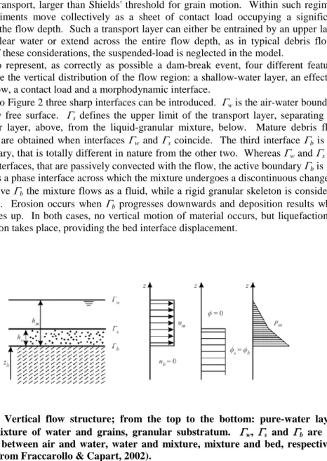
In order to represent, as correctly as possible a dam-break event, four different features characterize the vertical distribution of the flow region: a shallow-water layer, an effective mixture flow, a contact load and a morphodynamic interface.

Referring to Figure 2 three sharp interfaces can be introduced. Γw is the air-water boundary

at the flow free surface. Γs defines the upper limit of the transport layer, separating the

clear water layer, above, from the liquid-granular mixture, below. Mature debris flow conditions are obtained when interfaces Γw and Γscoincide. The third interface Γbis the

bed boundary, that is totally different in nature from the other two. Whereas Γwand Γsare

material interfaces, that are passively convected with the flow, the active boundary Γb is

modeled as a phase interface across which the mixture undergoes a discontinuous change of state. Above Γb the mixture flows as a fluid, while a rigid granular skeleton is considered

underneath. Erosion occurs when Γbprogresses downwards and deposition results when

the it moves up. In both cases, no vertical motion of material occurs, but liquefaction or solidification takes place, providing the bed interface displacement.

Figure 2 Vertical flow structure; from the top to the bottom: pure-water layer, flowing mixture of water and grains, granular substratum. Γw, Γs and Γb are the

interfaces between air and water, water and mixture, mixture and bed, respectively (adapted from Fraccarollo & Capart, 2002).

Appling the Reynolds transport theorem (e.g. see White 1999) to the balance of mass and momentum in a specific control volume the following integral equations can be obtained:

(31)

(

)

[

]

, 2 , 1 2 1 2 1

∫

+ − = Γ Γ ∂ ∂ b b b m m x x hmdx h u v e d t (1.19)

(

)

[

]

, 2 , 1 2 1 2 1

∫

+ − = Γ Γ ∂ ∂ b b b m s x x hsdx h u v e d t (1.20)

(

)

[

(

) (

)

]

, 1 2 , 1 2 1 2 1 2 2 1 2 2 1

∫

Γ Γ − = = + + − + + + ∂ ∂ b b bx w s m m m s m x x m s m d j rgh gh v u u rh h dx u rh h t ρ (1.21)

[

]

, 2 , 1 2 1 2 1

∫

+ − =− Γ Γ ∂ ∂ b b b b x x zbdx vz e d t (1.22) where:

• x and zb are, respectively, the horizontal and vertical coordinates;

• x1 and x2 are the lateral positions of the control volume boundaries;

• Γb1,2 is the portion of Γbinbetween the control volume;

• hm and hs are, respectively, the total depth over the bed boundary and the thickness

of the mixture layer (see Figure 2); • um is the horizontal mixture velocity;

• v is the non-material boundary velocity;

• g andρw are, respectively, the gravity acceleration and the water density;

• r = (s−1)φs is the density supplement due to the presence of the sediment load;

• ebis the erosion rate, i.e. the volume flux density across the bed interface Γb;

• jbx is the x-component of the momentum flux density across Γb;

• objects in squared parentheses give a jump across a discontinuity:

[ ]

f ₁2 = f₂− f₁. The above integral equations represent the flow layer continuity (1.19), the transport layer continuity (1.20), the horizontal flow momentum (1.21) and the conservation of mass applied to the solid bed substrate (1.22).

Assuming that shocks are absent, the flow is gradually varied and Γb is gently sloping, it is

possible to write the governing (simplified) equations in divergence form, by taking the limit x1→ x2:

(32)

(

)

,

(

)

, b, b b m s s b m m m e t z e u h x t h e u h x t h ₌₋ ∂ ∂ = ∂ ∂ + ∂ ∂ = ∂ ∂ + ∂ ∂ (1.23a,b,c)

(

)

(

)

(

)

(

)

, 2 2 1 2 2 1 2 w bn b s m s m m s m m s m x z rh h g rgh gh u rh h x u rh h t ρ τ − = ∂ ∂ + + + + + + ∂ ∂ + + ∂ ∂ (1.24)

where the erosion rate eb is given by:

(

) (

m bn

)

m w b u r e τ τ ρ + − = 1 1 , _(1.25)

while τbn and τm are the shear stresses acting on both sides of the bed interface Γb.

The system of divergence equations (1.23a,b,c) and (1.24) can be written in vector form as: ), ( ) (U U S U A U ₌ ∂ ∂ + ∂ ∂ x t (1.26)

where U is the vector of dependent variables, A(U) the Jacobian matrix and S(U) the source term vector.

By means of splitting procedures the system can be decomposed into three distinct components, each associated with a specific flow process. The flow hydrodynamics is described by the homogeneous PDE system, while geomorphic exchange and frictional momentum loss processes are represented with the two ODE systems:

, 0 ) ( = ∂ ∂ + ∂ ∂ x t U U A U (1.27) ) ( ), (U U F U G U e e _∂ = ∂ = ∂ ∂ t t (1.28a,b)

where the source vector S(U) has been split into two distinct components Ge(U) and Fe(U),

and the two equations associated with them represent, respectively, the geomorphic bed change driven by stress difference betweenτbn and τm and the frictional momentum loss due

to residual shear stress τbn.

New approximations, such as τbn = τm = 0, enable to arrange the equations, reducing the

(33)

, 0 3 , 0 = ∂ ∂ + ∂ ∂ = ∂ ∂ + ∂ ∂ + ∂ ∂ x u h t z x u h x h u t h m s s m w w m w _(1.29_a,b₎

(

)

(

)

(

)

(

)

0, 1 3 1 4 1 3 1 1 3 = ∂ ∂ + + + + + + ∂ ∂ + + + + + ∂ ∂ + + + + ∂ ∂ x u u h r h h r h x z g h r h h r h x h g h r h h h t u m m s w s w s s w s w w s w s w m (1.30)

where hw = zw − zs is the depth of the pure-water layer (see Figure 2), zs= zb+ hsand

g u hs m/

2 µ

= the elevation of the top of the sediment transport layer and its thickness (being µ a sediment mobility constant). Equations (1.29a,b) represent, respectively, a continuity equation for the pure- water layer and an Exner equation expressing conservation of the total sediment volume, while (1.30) is an equation of motion for the heterogeneous flowing mixture.

The vectorial form of such a system is:

, 0 ) ( = ∂ ∂ + ∂ ∂ x t W W B W (1.31) that forms a set of quasi-linear, first-order partial differential equations. The system solution moves through identification of the eigenvalues coming from matrix B.

The final solution can be found by solving the problem at hand as a typical Riemann problem.

(34)

Chapter 2. The numerical solver

As already mentioned, the NSWE are depth-averaged equations of conservation of mass and momentum which can be solved even when hydraulic jumps appear (e.g. see Whitham, 1974). A complete version of the NSWE, in a first instance, includes seabed friction. Indeed, the effects of seabed friction on nearshore dynamics are particularly significant both for near-shoreline flows and for longshore motions occurring in the surf zone, but their representation still poses many theoretical and practical problems. Formulations of the effects of bottom friction as a bulk frictional force, using semi-empirical formulae like the Chezy law, have generally been successful even for the oscillatory motions typical of the surf and swash zone (e.g. Longuet-Higgins, 1970; Watson et al., 1994).

The Exner equation models sediment conservation over the water column. The evaluation of the sediment fluxes there appearing is, probably, the most difficult aspect to be modeled. This difficulty also derives from the huge number of closure laws available to describe the sediment transport (e.g. Camenen & Larson, 2008). One common feature of almost all these laws is to distinguish the near-bed contribution to the sediment transport (bed-load) from contributions accounting for the transport of sediments spread outside the bottom boundary layer, all over the water column (suspended-load).

The NSWE/Exner system, written in conservative form, is a quasi-linear hyperbolic set of equations. The standard method for solving such a system is known as the “method of characteristics”. The “Riemann structure” of the fully-coupled system requires heavy computations for the eigenvalues and Riemann variables.

The novel solver here illustrated is based on a rather different perspective. It is supposed that the uncertainties related with the choice/use of appropriate sediment transport equations is so much higher than the eventual inaccuracies associated with the use of a weakly-coupled numerical solver that we have preferred to build a theoretical/numerical framework which enables a free choice of sediment transport laws and does not: i) rely on a specific sediment transport formula, ii) need to compute a specific characteristic wave structure.

Explicit writing and solution of the appropriate characteristic wave structure is only possible when very simple sediment transport laws are used (e.g. Kelly & Dodd, 2010). Theoretically, the drawback of the approach here proposed is a weak coupling between hydrodynamics (NSWE) and morphodynamics (Exner). However, it is shown that,

(35)

differently from what conjectured by some researchers (see Kelly, 2009 and Kelly & Dodd, 2010), a weakly-coupled model still captures all the main features of interest.

2.1. Splitting of the system and coupling issues

The fully-coupled system in its non-conservative form is: 0 ) ( ) ( + = + _x _y t ud vd d , _(2.1) d u C gz gd vu uu ut x y x x v τ − − = + + + , (2.2) d v C gz gd vv uv vt x y y y v τ − − = + + + , (2.3)

(

)

0 1 ₊ ₌ + _x _y t P Q z λ , (2.4) where:

• (x,y,z) are Cartesian orthogonal coordinates, being the still water level z=0; • d(x,y,t)=η(x,y,t)−z(x,y,t) is the water depth, with η(x, y, t) and z(x, y, t) being,

respectively, the free surface and the seabed position with respect to the still water level;

• v=(u,v) is the depth-averaged velocity vector (u(x,y,t) and v(x,y,t) being, respectively, the onshore and longshore components);

• Q=(P,Q) is the sediment transport flux (P and Q being, respectively, the onshore and longshore components);

• Cτ is the dimensionless Chezy coefficient (typically of order 10-2);

• λ=1-p is the grain packing (typically 0.5≤λ≤0.8), being p the beach porosity; • g is the gravity acceleration;

• subscripts represent partial differentiation.

The geometrical terms presented in the previous equations are sketched in Figure 3, where a typical seabed evolution is shown.

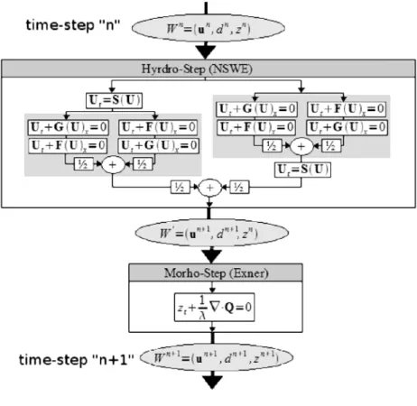
An operational split solution of the NSWE/Exner system is achieved by separately solving the NSWE and Exner equations. The NSWE system is solved by using the WAF method, well described in §2.2.3, whose scheme is here labeled as H. The Exner system is solved by using a “finite-volume” method, described in §2.3.2, whose scheme is here labeled as M. The splitting scheme, which is a first-order accurate in time split operator, gives, from the initial solution Wn=(dn,un,vn,zn), the solution at the following time-step Wn+1 through the relation:

(36)

( )

(

n

)

n W H M W +1= . (2.5)

A detailed flow chart of the integration procedure is provided in Figure 4.

In all the document, superscript n represents the time index while i, j represent space grid point indices referring, respectively, to the x and y coordinates.

Figure 3 Sketch of seabed profile and free surface elevation.

2.2. The hydrodynamic solver

The hydrodynamic solver is that developed by Brocchini et al. (2001). It uses a conservative finite-volume discretization method to take into account discontinuous solutions (e.g. shock waves) by means of an appropriate flux method. A TVD scheme is also applied by using a flux limiter to avoid spurious oscillations due to discontinuous solutions.

(37)

Figure 4 Flow chart of the computational schemes.

2.2.1. System resolution

The vectorial conservative form of the NSWE is:

( )

U G

( )

U S

( )

U

F

Ut+ x+ y = , (2.6)

(38)

( )

, , 1 3 2 1 2 2 2 1 2 1 2 2 2 1 2               + =           + =           = U U U U U gU U uvd gd d u ud vd ud d U F U

( )

, 0 , 2 1 2 1 3 2 2 1 2 1 2 3 1 3 2             − − − − =               + =             + = v C gdz u C gdz gU U gd d v uvd vd y x U U U U U v v U S U G τ τ (2.7)

with z constant in time.

The system (2.6) is split to have two 1D-homogeneous equations and a “source” equation:

( )

=0 + _x t FU U , (2.8)

( )

=0 + _y t GU U , (2.9)

( )

U S Ut = . (2.10)

The global hydrodynamic scheme, which is a combination of two symmetrical second-order schemes, can be described as follows. If Hx is the scheme which solves (2.8) over the time dt=tn+1−tn, Hy the scheme which solves (2.9) and So the scheme which solves (2.10), the numerical procedure that leads from the initial condition Un to the solution Un+1 can be described as follows:

( )

(

)

(

( )

)

(

n n

)

n H So So H U U U + = + 2 1 1 , (2.11) where

( )

n

(

( )

n

)

(

( )

n

)

Hx Hy Hy Hx H U = U + U 2 1 . (2.12)

2.2.2. Integration: finite-volume discretization

The rectangular domain S=[xi-1/2, xi+1/2]×[tn, tn+1] in the x-t space is the fundamental unit

used to discretize the computational domain (see Figure 5).

An integral form of these equations has been used over the rectangular volume S. For instance, equation (2.8) becomes:

(39)

( )

[

]

(

,

)

( )

,

(

,

)

(

,

)

0. ) ( 2 / 1 ) ( 2 / 1 ) ( ) ( 1 1 1 2 / 1 2 / 1 2 / 1 2 / 1 = − + − = = +

∫

+ + + − + − − + +                           D t t i C t t i B x x n A x x n S t x n n n n i i i i dt t x dt t x dx t x dx t x ds F F U U U F U (2.13)

The “cell averages” can be defined as:

, ) ( , ) ( , ) ( , ) ( 1/2 2 / 1 2 / 1 2 / 1 1 t C t D x A x B n i n i n i n i = _∆ U + = _∆ F−+ = _∆ F++ = _∆ U (2.14)

where Δx = xi+1/2− xi-1/2and Δt = tn+1− tn.

Substitution of the averages into (2.13) gives:

(

1/2

)

2 / 1 2 / 1 2 / 1 1 + + + − + ₋ ∆ ∆ + = n i n i n i n i x t F F U U . (2.15)

Figure 5 Sketch of the domain S in the x−t space.

2.2.3. The WAF method

At this stage a suitable method is needed for representing the flux terms in (2.15) and then for solving the equation. To have a good approximation even when shocks occur, the WAF (Weight Average Fluxes) method is used.

The WAF method requires knowledge of the “Riemann structure” of the equations to be solved.

(40)

At the intercell boundary xi+1/2and at time level n, we can define a special initial value

problem called “sub-grid Riemann problem” with initial conditions (UL, UR).. For equation

(2.8), this reads:

( )

    > = < = = = = + = + + + + 2 / 1 1 2 / 1 0 if , if , ) ( ) 0 , ( , 0 i n i R i n i L x t x t x x x x x x U U U U U U AU U U F U , (2.16)

The characteristic curves of the solution are determined through the eigenvalues of the matrix A=∂F/∂U, then suitable multipliers are found to decouple the set of PDEs of (2.16) in a set of ODEs along which Riemann variables R propagate. In absence of source terms for the ODEs, they propagate unaltered according to:

1,2,3 where , along 0 = = = k dt dx dt d k k _λ R , (2.17)

and are the “Riemann invariants”. Eigenvalues are: (λ1, λ2, λ3) = (u−c, u, u+c) , with

gd

c

=

, while the Riemann invariants are (R1, R2, R3) = (u−2c, v, u+2c).

Hence, the structure of the solution of the specific Riemann problem reveals the presence of two known constant states, UL and UR, and two unknown states, U*L and U*R, as also shown in Figure 6.

Values of U*L and U*R are taken as constant in agreement with the approach used by Toro (1997). Hence, neglecting the overbar sign, because variables are piece-wise constant (within each cell), the intercell vector is defined as:

                < < = = < < = < < = < < = = = + + + + + + + 4 3 3 2 2 1 1 0 A A 2 / 1 1 A A 2 / 1 A A 2 / 1 A A 2 / 1 2 / 1 2 / 1 , for , for * , for * , for x x x t t x x x t t x x x t t x x x t t n n i R n R n L n n i L n i U U U U U U U . (2.18)

The operative value of the intermediate flux

F

_i₊n₁+1_/₂/2 is estimated by the weighted average (hence the name WAF) of the F(U) values of equation (2.18). This can be accomplished by introducing the length of each segment

A

_k₋₁

A

_k , appearing in Figure 6, normalized by the cell width Δx:

β

_l

=

A

_k₋₁

A

_k

∆

x

, with l=1,4. Hence:

(41)

. 2 2 1 , 2 2 , 2 2 , 2 2 1 3 4 3 2 3 2 1 2 1 1 x t x t x t x t ∆ ∆ + = ∆ ∆       ₋ = ∆ ∆       ₋ = ∆ ∆ − = λ β λ λ β λ λ β λ β (2.19)

Thus, the following weighted average fluxes are obtained:

( )

( ) ( )

(

_{) ∑}

= ± + ± + + + ∆ − + = ⇒ + + + = 3 1 ) ( 1 2 / 1 2 / 1 1 4 3 2 1 2 / 1 2 / 1 2 1 2 1 * * l l l n i n i n i n i R L n i n i C F U F U F F U F U F U F U F F β β β β (2.20)

ΔF(l) being the flux jump across the lth wave and Cl = λl Δt/Δx the Courant number of each

wave.

Figure 6 Flux computation from one specific Riemann problem in the x−t space. Finally, generation of spurious oscillations caused by strong gradients is prevented by using a Total Variation Diminishing (TVD) version of equation (2.20) (see Harten, 1983). This is obtained by means of the SUPERA flux limiter function (Toro, 1997)

f

_ln_i_±+₁1_//₂2such that:

(42)

( ) ( )

(

)

_∑

( )

= + ± ± + ± = + − ∆ 3 1 ) ( 2 / 1 2 / 1 1 2 / 1 2 / 1 2 1 2 1 l l n i l l n i n i n i FU FU signC f F F . (2.21) 2.2.4. Shoreline treatment

The treatment of the shoreline motion is really important to model properly the intermittent flow caused by wave motion on a beach (e.g. see Brocchini et al. 2001; Brocchini & Peregrine, 1996). In the present work a wetting/drying approach is used to predict the shoreline motion.

The first step consists in the computation of an equivalent water depth for each cell by considering the inflow volume, that is the sum of all contributions occurred during the previous time-steps. Then (Stoker, 1957) the WAF method is applied to the sub-grid Riemann problem occurring at the shoreline, by evaluating the equivalent depth in each cell as a function of the water level at the nodes around it.

If the equivalent depth is larger than a threshold value dmin, the cell becomes wet. During

the drying phase, if the water depth is lower than dmin, the cell becomes dry and the water

depth is set equal to zero. Since the shoreline is the interface between wet and dry cells, the shoreline boundary condition can be written as:

0 , = = _s _s s d dt dx v (2.22)

where xs is the position of the instantaneous shoreline, vs and ds the flow velocity and the

water depth at the shoreline, respectively.

The Riemann problem that is considered to solve (2.22) is defined right at the edge between the last “wet grid point” xi and the first “dry grid point” xi+1. It is similar to that modeling a

moving piston (see Stoker, 1957) which represents the shoreline advancing, as shown in Figure 7 and described by:

( )

= + =0, ( ,0)= if < +1/2 + L _i x t x t FU U AU U x U x x U . (2.23)

Equations for the motion of the shoreline are obtained by determining the value of us for

which the constraint ds = 0 is satisfied. After some calculations, it can be obtained us = uL+2cL with cL = gdL . The smooth transition between the left state and the shoreline can be described by: [~,~] [ /2,( s)/2]

L L u u d u

(43)

Figure 7 Sketch of the solution of the shoreline Riemann problem and analogy with the moving piston.

Finally, the flux at the shoreline boundary is:

(

)

(

)

      ₊ ₋ ∆       ∆ ₊∆ ∆ = + + F F F ~ 2 , 2 2 1 1 1 2 / 1 2 / 1 t u d x t x s L L n i λ λ λ . (2.24)

The expansion fan contribution is

F

~

, defined as:

(

)

( )

(

s

)

L L u u d u d 0, 4 1 ~ , ~ 2 1 , 4 1 ~ F F F F= + + , (2.25) where λ1=uL−cL and λs=us.

2.3. The morphodynamic solver

The morphodynamic solver has been developed to properly match the hydrodynamic solver which provides the forcing to update (2.4) in time. To be consistent with the hydrodynamic solver, many of its features have been employed in the morphodynamic resolution, e.g. the finite-volume approach.

NUMERICAL HYDRO- MORPHODINAMIC 2DH MODEL FOR THE SHALLOW WATERS

NUMERICAL

HYDRO-MORPHODINAMIC 2DH MODEL

FOR THE SHALLOW WATERS

Ph.D. Dissertation of:

Matteo Postacchini

NUMERICAL

HYDRO-MORPHODINAMIC 2DH MODEL

FOR THE SHALLOW WATERS

Ph.D. Dissertation of:

Matteo Postacchini

Acknowledgements

Abstract

Contents

Contents... i

List of Figure

s ... iii

List of Tables ... v

Chapter 1. ... 1

Introduction ... 1

1.1.

Wave dynamics in the nearshore zone ... 1

1.2.

The modeling of the nearshore sediment transport... 2

1.3.

The coupling issue ... 5

Chapter 2. ... 15

The numerical solver ... 15

2.1.

Splitting of the system and coupling issues ... 16

2.2.

The hydrodynamic solver ... 17

2.3.

The morphodynamic solver ... 24

2.4.

Numerical instabilities and filtering ... 28

Chapter 3. ... 31

The experimental tests ... 31

3.1.

The experimental set up ... 31

3.2.

Salient morphological results ... 35

Chapter 4. ... 39

Validation of the numerical solver ... 39

4.1.

Validation of the bed-load transport: Fraccarollo & Capart (2002) 40

4.2.

Validation of the bed-load transport: Kelly (2009) ... 45

4.3.

Validation of the suspended-load transport: Pritchard & Hogg

(2005)

49

4.4.

Validation of the total transport: flume experiments ... 54

Chapter 5. ... 64

Concluding Remarks ... 64

References ... 68

Appendix A. ... 71

The theoretical approach in the laboratory experiments ... 71

Appendix B. ... 73

List of Figures

List of Tables

Chapter 1.

Introduction

1.1.

Wave dynamics in the nearshore zone

1.2.

The modeling of the nearshore sediment transport

1.3.

The coupling issue

(

)

ξ

=

1

(

1

−

p

)