Parallel Brownian Dynamics Simulations with the
Message-Passing and PGAS Programming Models
C. Teijeiroa,∗, G. Sutmannb,c, G.L. Taboadaa, J. Touri˜noa
a
Computer Architecture Group, Department of Electronics and Systems, University of A Coru˜na, 15071 A Coru˜na, Spain
b
J¨ulich Supercomputing Centre, Institute for Advanced Simulation, Forschungszentrum J¨ulich, D-52425 J¨ulich, Germany
c
ICAMS, Ruhr-University Bochum, D-44801 Bochum, Germany
Abstract
The simulation of particle dynamics is among the most important mecha-nisms to study the behavior of molecules in a medium under specific condi-tions of temperature and density. Several models can be used to compute efficiently the forces that act on each particle, and also the interactions be-tween them. This work presents the design and implementation of a parallel simulation code for the Brownian motion of particles in a fluid. Two dif-ferent parallelization approaches have been followed: (1) using traditional distributed memory message-passing programming with MPI, and (2) using the Partitioned Global Address Space (PGAS) programming model, oriented towards hybrid shared/distributed memory systems, with the Unified Paral-lel C (UPC) language. Different techniques for domain decomposition and work distribution are analyzed in terms of efficiency and programmability, in order to select the most suitable strategy. Performance results on a super-computer using up to 2048 cores are also presented for both MPI and UPC codes.
Keywords: Brownian dynamics, parallel simulation, MPI, PGAS, UPC
2000 MSC: 60J65 (Brownian Motion), 68U20 (Simulation), 68W10 (Parallel Algorithms)
∗Corresponding author
Email addresses: [email protected](C. Teijeiro),[email protected](G. Sutmann),[email protected](G.L. Taboada),[email protected](J. Touri˜no)
1. Introduction
Dynamical particle simulations aim at exploring the phase or configura-tion spaces of the underlying physical system in order to gather statistics for the calculation of expectation values of observables. Depending on the
level of resolution either ab initio methods, force field or effective medium
descriptions are used to propagate particles according to their equations of motion. Interactions between solvated particles as well as particle-solvent-and particle-wall-interactions are modeled according to their physical cha-racteristics, their statistical properties and information from experimental data. Brownian dynamics is a class of simulation that takes into account the systematic interactions between particles, as well as the interaction with a surrounding medium described by their statistical and transport properties, which are often represented by diffusion tensors derived from a velocity field description of the solvent.
It is assumed that solvated particles are very large compared to fluid particles and that individual interactions can be reduced to statistical fluc-tuations, induced by thermal noise. This allows to consider a time scale separation, i.e. during a time step in which a so called Brownian or solute particle is propagated (e.g., macromolecules, polymers or colloids), individual solvent particles would perform a large number of micro steps and therefore the fluid-solute interaction is considered as an average action. Thus, although individual interactions between fluid and solute are not considered, the simu-lation takes into account the collective properties of the fluid molecules using a mobility tensor, which contains information about the velocity field in the system.
Technically, a finite difference scheme is applied to calculate the trajectory for each particle as a succession of short displacements ∆t in time. In a system, containing N particles, the trajectory {ri(t);t∈[0, tmax]}of particle
i is calculated as a succession of small and fixed time step increments ∆t.
The time step is selected thereby: (1) large enough with ∆t ≫ mi/6πηai,
with η the solvent viscosity, ai the radius and mi the mass of the solute
particle i, so that the interaction between individual fluid particles and the solutes can be considered as averaged and can be coupled to the solutes via the diffusion tensor, and (2) small enough so that the forces and gradients
of the diffusion tensor can be considered constant within ∆t. According to
these conditions, the simulation can be performed by calculating the forces that act on every particle in a time step, determining new positions for all
particles and continuing this process in the following time step.
Brownian dynamics simulations are nowadays used to perform many stud-ies in different areas of physics and biology [1], and there are several software tools that help implementing these simulations, such as BrownDye [2] and the BROWNFLEX program included in the SIMUFLEX suite [3]. Some relevant work has also been published on parallel implementations of these simulations on GPUs [4], also including a simulation suite called BD BOX [5]. However, there is still little information on parallelization methods for these simulations, especially about their performance and scalability on high per-formance computing (HPC) systems. This work overcomes these limitations by providing an accurate description of the parallelization of a Brownian dy-namics simulation for a set of solvated particles in a certain period of time, in order to build a suitable implementation for HPC systems. The paral-lel algorithm has been developed using MPI and Unified Paralparal-lel C (UPC), which illustrate two programming models, message-passing and Partitioned Global Address Space (PGAS), respectively, to obtain high efficiency and scalability. The most relevant information about the parallelization of the different parts of the simulation is presented, and its performance is analyzed on a supercomputer in order to explain the behavior of the code for different test cases.
The rest of this work is organized as follows. First, Section 2 presents the formal explanation of the simulation. Section 3 contains a detailed com-putational description of the simulation code. In Section 4 details about the parallelization strategies are outlined, and Section 5 presents performance results of the parallel codes using different workloads and computational re-sources. Finally, Section 6 extracts the main conclusions from this work.
2. Theoretical background of Brownian dynamics
The equation of motion, governing Brownian dynamics for solvated mo-lecules in a fluid, has been stated by Ermak and McCammon [6] (based on the Focker-Planck and Langevin descriptions):
ri(t+ ∆t) =ri(t) + N X j=1 ∂Dij(t) ∂rj ∆t+ N X j=1 1 kBT Dij(t)Fj(t)∆t+Ri(t+ ∆t) (1) This one-step propagation scheme takes into account the coupling of the particles to the flow field via the diffusion tensorD∈R3N×3N and the
system-atic forces F, acting onto the particles with the global property P
j Fj = 0.
The vector R ∈ R3N contains correlated Gaussian random numbers with
zero mean, which are constructed according to the fluctuation-dissipation theorem, i.e.:
hRi,αi= 0 , α=x, y, z (2)
hRi(t+ ∆t)RTj(t+ ∆t)i= 2Dij(t)∆t (3)
with Ri ∈ R3 and Dij ∈ R3×3, being sub-vectors and block-matrices corre-sponding to particleiand particle pairs i, j, respectively. kBT is the thermal
energy of the system, where T is the temperature andkB the Boltzmann
con-stant. Depending on the approximation for the diffusion tensor, the partial derivative on the right-hand side of Eq. 1 might drop out. This is the case e.g. of the Oseen tensor and the Rotne-Prager tensor [7, 8]. The latter one takes into account the finite size of solute particles, and its regularized version is considered in the present work [7], thus fulfilling the requirement of positive definiteness also for inter-particle distances rij < 2a where rij = kri −rjk. Here, we give the expression for the so called minimum image convention. The expression for periodic boundary conditions applied in the code is out-lined in Appendix A. The minimum image formulation is given by:
Dii= kBT 6πηaI (4a) Dij = kBT 8πηrij I+ˆrijˆrTij + 2 3 a2 r2 ij I−3ˆrijˆrTij : rij >2a kBT 6πηa 1− 9 32 rij a I+ 3 32 rij a ˆrijˆr T ij : rij ≤2a (4b)
where ˆrij = (ri −rj)/rij. Applying this form of the diffusion tensor, the displacement vector of the Brownian particles, ∆r=r(t+ ∆t)−r(t), can be rewritten in a more simple way:
∆r= 1
kTDF∆t+
√
2∆tZξξξ (5)
whereξξξ is a vector of independent Gaussian random numbers. According to
Eq. 3, the relation R = √2∆tZξξξ holds with D = ZZT, which relates the
stochastic process to the diffusion matrix. Therefore, Z may be calculated
are very CPU-time consuming with a computational complexity of O(N3)
and impose a large computational load. Therefore the development of faster and more efficient and scalable methods with smaller complexity is an im-portant task, in order to overcome the limitations in the system size. Such an approach was introduced by Fixman [9], who applied an expansion of
the random displacement vector R in terms of Chebyshev polynomials,
ap-proximating its values without constructing Z explicitly and reducing the
computational complexity to O(N2.25).
Both methods for the construction of correlated random variates, based on the Cholesky decomposition and the Chebyshev approximation, will be considered in the present work.
3. Implementation of the simulation code
The Brownian dynamics simulation has been initially implemented in se-quential C code. The system under study consists of a cubic box where periodic boundary conditions are applied, and the propagation of Brownian particles is performed by evaluating Eq. 5. The systematic interactions be-tween particles are modeled by a Lennard-Jones type potential, from which the forces are obtained via the negative gradient:
V(rij) = 4ε " σ rij 12 − σ rij 6# (6a) Fij =−∇rijV(rij) = 24ε " 2 σ rij 12 − σ rij 6# ˆrij r2 ij (6b)
where σ is the diameter of the particles and ǫ is the depth of the potential
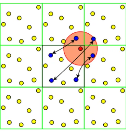
minimum. This potential has a short range character and practically inter-actions between particles are neglected for mutual distances rij > Rc, where Rc is the radius of a so called cutoff sphere, which is chosen as Rc = 2.5σ.
The distance rij is chosen according to the minimum image convention, i.e.
the shortest distance between particle i (located in the central simulation
box) and particle j or one of its periodic images is taken into account (see
Fig. 1). In the code, the diffusion tensor D is calculated in periodic images,
which implies a summation of particle pair contributions over all periodic images. The expression, which consists of a splitting into a short and long range contribution, is given in Appendix A. Depending on the parameters
Figure 1: Example of the short range interaction model with periodic boundary conditions
κ, kmax, Rc,D in Eqs. A.3a-A.3d, which are determined by the required
ac-curacy and optimal runtime performance, the short range part of D might
exceed half of the box length (Rc,D > L/2), which makes it formally nec-essary to test explicitly all nearest periodic images of particle j, whether or not it contributes to D.
The main component of the code is aforloop. Each iteration of this loop
corresponds to a time step in the simulation, which calls several functions,
being calc force() and covar() the most time consuming among them
and thus the main targets of the parallelization. Function calc force()
in-cludes: (1) the propagation of particles (with O(N) complexity, where N is
the number of particles in the system), (2) the force computation, for which a linked-cell technique [10] is used (O(N)), and (3) the setup of the diffu-sion tensor (O(N2)). The correlated random displacements are calculated in
function covar() via a Cholesky decomposition (O(N3)) and alternatively
via the Fixman’s approximation method, with complexity O(N2.25) [9].
The values of the diffusion tensor D are computed in calc force() for
every pair of particles in the system according to the distance between them in every dimension following the Rotne-Prager tensor description, and then
stored using double-precision floating point values in matrix D, which is
de-clared as a square pNDIM×pNDIM matrix, where pNDIM is the product of the
total number of particles (N) and the system dimensions (3). Thus, each
row/column in D is associated to a particle and a dimension (for example,
valueD[3*4+2][3*8+2] contains the diffusion tensor between particles 4 and
8 in the third dimension,z). The interaction values inD[a][b]are also stored in D[b][a], being D symmetric, i.e. the values of the upper triangular part
of D are computed and they are copied to the corresponding positions in the lower triangular part. This data replication has several advantages for the sequential algorithm because it helps simplifying the implementation of the
operations with matrix D, allowing more straightforward computations on
this matrix.
After the initialization ofDincalc force(), functioncovar()calculates
the random displacement vector R, which requires the construction of
cor-related Gaussian random numbers with given covariance values (Eq. 3). As stated in Section 2 (see Eq. 5), the random vector is written as:
R=√2∆tZξξξ (7)
where the random valuesξξξ are obtained using the pseudo-random generator
rand() (a Box-Muller method [11] may also be used here), and Z can be
obtained either as a lower triangular matrixLfrom a Cholesky decomposition
or as the matrix square root S.
To obtain the entries of matrix L, the following procedure is applied:
Lii= v u u tDii− i−1 X k=1 L2
ik , for diagonal values in L (8a)
Lij = 1 Ljj Dij − j−1 X k=1 LikLjk ! , where i > j (8b)
The random vector is then obtained via the following steps:
D= D11 D12 ··· D1n D21 D22 ··· D2n ... ... ... ... Dm1 Dn2 ··· Dnn Cholesky −→ L= L11 0 ··· 0 L21 L22 ··· 0 ... ... ... ... Lm1 Ln2 ··· Lnn L matrix-vector−→ Ri = √ 2∆t i X j=1 Lijξj (9)
i.e. having calculated the diffusion tensor matrixD, a Cholesky decomposition
generates the lower triangular matrix L, from where R is generated via a
The alternative to this method is the use of Fixman’s algorithm, which
implements a fast procedure to approximate the matrix square root S using
Chebyshev polynomial series. The degree of the polynomial is fixed depend-ing on the desired accuracy for the computed values. The advantage of this
method is that it does not need to build the matrix S explicitly, but
con-structs directly an approximation to the productSξξξ in an iterative way. The computations performed here represent a generalization of known series to obtain the scalar square root to the case of vectors:
SM = M
X
m=0
amCm (10a)
where M is the degree of the polynomial, which controls the accuracy of
approximation. In the limit it holds that limM→∞SM =S. Accordingly, the
vector of correlated Gaussian variates becomes:
ZM =SMξξξ = M X m=0 amCmξξξ = M X m=0 amzm (10b)
The coefficients am can be pre-computed [12] and the vectors zm are
com-puted within an iterative procedure:
z0 =ξξξ ; z1 = (daD+dbI)ξξξ ; zm+1 = 2 (daD+dbI)zm−zm−1 (11a) with da= 2 λmax−λmin ; db = λmax+λmin λmax−λmin (11b)
where λmin, λmax are the upper and lower limits for the eigenvalues of D.
For more details, see references [13, 14].
The approximation vectors zm, as well as the maximum and minimum
eigenvalues of D, are computed analogously using two separate iterative
al-gorithms. These algorithms apply the technique of double buffering, i.e. use a pair of arrays that are read or written alternatively on each iteration: every approximation (associated to a particle in a dimension) is computed using all the approximated values from the previous iteration, therefore the use of two arrays avoids additional data copies and data overwriting. This procedure will be illustrated in Section 4.4.2.
After computing the random displacements in an iteration, the function
the force vectorF, and adds all the computed contributions to obtain the new positions of the particles (reduction operation). The matrix-vector product
has O(N2) complexity for this function. Some additional physical values,
e.g. pressure, are also computed here to monitor and control the progress of the simulation.
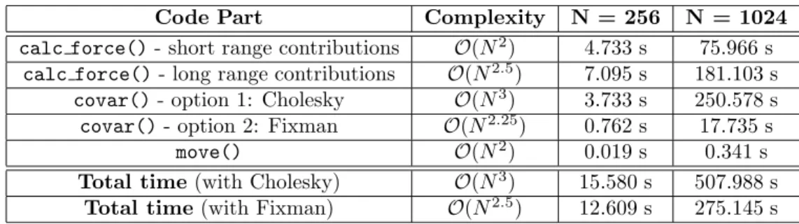
Table 1 presents the breakdown of the execution time of the sequential program in the testbed used in the performance evaluation (see Section 5) in terms of the previously discussed functions, using 256 and 1024 input
particles for 50 time steps of simulation. The diffusion tensor matrix D has
(3×N)2elements, thus its construction takes at least a complexity ofO(N2).
This is true for the real space contributions of the Ewald sum as the cutoff radius is of the order of half the system size (or even larger), in order to keep the reciprocal space contribution, i.e. the number of k-values, small for a given error tolerance.Since the mutual distances between particles are calcu-lated in the real space contribution, it is natural to integrate the construction of matrixD in the calculation of short range direct interactions between par-ticles (whose complexity is O(N)), thus giving out the O(N2) complexity
stated in row “short range contributions” of Table 1. The long range con-tribution to the diffusion tensor also has to be calculated for every matrix element, i.e. for each particle pair, which also imposes a computational com-plexity of O(N2). However, there is an additional contribution to the long range part, giving rise to a larger complexity, since a set of reciprocal vectors (cf. Appendix A) has to be considered to fulfill a prescribed error tolerance in the Ewald sum, increasing the complexity to approximately O(N2.5). The
computations of covar() also tend to reveal the different complexities of
Cholesky decomposition and Fixman’s algorithm commented in Section 2.
Code Part Complexity N = 256 N = 1024
calc force()- short range contributions O(N2
) 4.733 s 75.966 s
calc force()- long range contributions O(N2.5
) 7.095 s 181.103 s
covar()- option 1: Cholesky O(N3
) 3.733 s 250.578 s
covar()- option 2: Fixman O(N2.25
) 0.762 s 17.735 s
move() O(N2
) 0.019 s 0.341 s
Total time(with Cholesky) O(N3
) 15.580 s 507.988 s
Total time(with Fixman) O(N2
.5) 12.609 s 275.145 s
4. Building the parallel implementation
The strong increase with the number of particles of the total execution time is the main motivation for the development of a parallel implementation of this code. Two approaches have been followed: (1) the use of a message-passing programming model with the MPI C library, and (2) the use of a parallel language, PGAS UPC [15], which extends ANSI C for parallel processing.
The MPI library represents a traditional and widely used approach for
parallel programming, and nowadays is the de facto standard for
program-ming distributed memory architectures. Several mature and optimized im-plementations of MPI are currently available (e.g., MPICH2 and Open MPI), with bindings for multiple languages (C, Fortran and C++), making it suit-able for the parallelization of this application.
However, MPI presents several limitations when programming hybrid shared/distributed memory architectures, such as clusters of multi-core pro-cessors, as well as scalability issues because of the two-sided nature of its communications. Looking for alternatives to MPI, UPC has been selected to develop another parallel simulation code that would potentially take more advantage of the growing complexity of current multi-core systems. The ar-chitectural improvements in these systems (e.g., the increasing number of cores per processor, the use of improved cache coherence mechanisms or heterogeneous components) imply higher complexity in code development in order to exploit all resources efficiently, and here traditional parallel pro-gramming approaches tend to provide either low programmability (e.g., MPI) or low flexibility (e.g., OpenMP). As a result, new programming paradigms have been proposed to adapt to new computer architectures, among which PGAS has been attracting the attention of many developers in the last years. The UPC language, based on the PGAS memory model, provides a global view of a memory space shared by all threads, while accessing data effi-ciently through a logical partitioning of the memory among threads. Each one of these shared memory portions is said to have affinity to a particu-lar thread, and all computations of a given thread in its associated memory space will benefit from data locality. UPC provides several constructs to exploit PGAS features, such as: (1) the definition of shared variables that allow implicit data transfers via direct assignments, (2) a loop construct that
distributes the work in different iterations between threads (upc forall),
and MYTHREAD (thread identifier), and (4) a collection of standard libraries which include one-sided memory transfers and collective functions, among others.
4.1. Parallel workload decomposition
A preliminary analysis of the structure of the simulation code reveals that each iteration of the main loop, i.e. each time step, has a strong de-pendence on the previous iteration, because the position of a particle in an instant of time depends on calculations performed in the previous time step. Therefore, these iterations cannot be executed concurrently, so the work dis-tribution is only possible within each iteration. At this point, the main parallelization efforts have to be focused on the workload decomposition of
calc force(), according to Table 1, but also considering the performance bottlenecks that might arise when performing communications, especially at the covar() function.
In order to allow the parallel computations needed to update the diffusion tensor values and random displacements, all processes (for clarity purposes, the term “processes” will be used when considering both MPI processes and UPC threads) require to have access to the coordinates for every particle in the system. Thus, all processes store all the initial coordinates of the particles to avoid continuous remote calls to obtain the necessary coordinate values. After each iteration, all coordinates are updated for every process
by means of function move(), thus minimizing communications. Moreover,
this assumption allows the parallel computation of short and long range con-tributions without involving any communication: each process can compute
any element of matrix D independently from the rest, and therefore the
par-allelization of calc force() becomes straightforward. The tradeoff of this
approach is a slightly higher memory consumption (approximately pNDIM
double-precision additional values).
However, the computation of each random displacement in covar()
de-pends on many of the elements of matrixD, whose computation has been
pre-viously performed by different processes in calc force(), and consequently
communications are unavoidable here. Therefore, it is necessary to find a
suitable workload distribution of diffusion tensor values in matrix D to favor
the scalability of the code by minimizing the amount of communications
re-quired bycovar(). The following subsections present different approaches to
increase the scalability of the code taking advantage of the specific features of MPI and PGAS UPC.
4.2. Shared memory direct parallelization
The use of the UPC shared memory region to store matrix D allows a
straightforward shared memory parallelization, as shown in Figure 2 for 4 threads using a sample matrix, divided in four chunks of equal size (one per thread). Each element on it represents the diffusion tensor values associated to a pair of particles in every combination of their dimensions, that is, a
3×3 submatrix. In UPC, all threads are able to access all the data stored
in the shared memory region, so this parallelization only requires changes in the matrix indexing to support the access in parallel by UPC threads.
Here, the matrix is distributed in blocks of N/THREADS elements (i.e., 3 ×
3 submatrices) among threads. Each diffusion tensor value from the upper triangular part of the matrix is computed by the thread to which it has affinity (see left graph). After that, the upper triangular part is copied into the lower triangular part (see right graph) as described in Section 3, using implicit one-sided transfers initiated by the thread that has the source data by means of assignments.
THREAD 0
THREAD 1
THREAD 2
THREAD 3
Local data movement Remote data movement shared [ pNDIM*pNDIM / THREADS ] double D [pNDIM*pNDIM]
Figure 2: Work and data distribution withDas a shared matrix in UPC
This approach has allowed the quick implementation of a prototype of the parallel code, providing a straightforward solution for distributed memory architectures thanks to the shared memory view provided by UPC. This represents a significant advantage over MPI, where the development of an equivalent version of this parallelization would require a significantly higher programming effort because of the lack of a shared memory view (data have to be transferred explicitly among processes), showing poorer productivity.
However, there are two drawbacks in this parallelization. The first one is its poor load balancing: thread 0 performs much more work than the
last thread (THREADS-1). This workload imbalance can be partly alleviated through the distribution of rows in a cyclic way, but this will not be enough when the number of threads is large and few rows are assigned to each thread. The second issue of this work distribution is the inefficiency of single-valued remote memory copies [16], which is due to the use of virtual memory ad-dresses to map the shared variables in UPC. While private variables have addresses that are directly translated to physical positions in memory, shared variables use an identifier that includes information about the thread to which the variable has affinity, the data block to which it belongs (in arrays, this can be defined with a block size parameter) and the offset of the variable inside the data block. As a result, the computational cost of handling these shared address translations is not acceptable when simulating large systems for a long period of time.
4.3. Private distributed memory parallelization
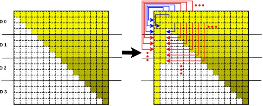
Figure 3 presents the distribution of matrix D and its associated data
movements for a more balanced workload decomposition on private dis-tributed memory, where each process is assigned a set of particles in the system in order to compute their corresponding diffusion tensor values. Here the number of particles associated to a process is not evenly divided, but instead follows an analogous approach to the force-stripped row decomposi-tion scheme proposed by Murty and Okunbor [17], with the goal of achieving
a more balanced number of computations and remote copies in matrix D.
This workload/domain decomposition consists in distributing the number of
elements in the upper triangular part of matrixD (pNDIM×(pNDIM+1)/2,
de-fined asnelemsin the code) between the number of processes in the program
by assigning consecutive rows to processi until the total number of assigned
diffusion tensor values is equal to or higher thannlocalelems*(i+1), where
nlocalelems isnelems divided by the number of processes.
This approach has been implemented both in MPI and UPC. In both scenarios, first all computations of diffusion tensor values are performed lo-cally by each process, and then the values are moved to the corresponding
destination in the lower triangular part of matrix D. Sometimes the
desti-nation position is local to the process which has the source data (see local data movements in the middle graph of Figure 3), whereas on the remaining cases there are data transfers between processes (see remote data movements in the right-most graph of Figure 3). Regarding the UPC parallelization,
PROCESS 0
PROCESS 1
PROCESS 2
PROCESS 3
Local data movements Remote data movements
Figure 3: Balanced workload decomposition of Don private distributed memory
for each submatrix. The reason for this decision is that the UPC standard does not allow the allocation of a different number of elements per thread in the shared memory region, i.e. the block size of a shared array must be the same for all threads.
Despite the relatively good balancing of this distribution, its main draw-back is the significant overhead associated to the communications needed
to achieve the symmetry in matrix D. After obtaining the symmetric
ma-trix, the next step in the simulation (function covar()) involves either a
Cholesky decomposition or a Fixman approximation. The Cholesky decom-position can take advantage of the previous matrix distribution, minimizing the number of remote communications. Regarding Fixman’s algorithm, it
is really convenient to fill the lower triangular part of matrix D in order to
avoid smaller element-by-element data movements in covar(), but the
com-munication time may become too high even when few processes are used. This is also confirmed by the results of Table 1: the sequential computation of the interactions for 1024 particles takes less than 5 minutes for 50 time steps, being the average calculation time of each tensor value of about 0.6 microseconds in each iteration, and after that a large percentage of these computed values is remotely copied (about 68% in the example in Figure 3). As a result, the cost of communications can easily represent a significant percentage of the total execution time.
4.4. Optimization of the parallel implementation
An analysis of the previously presented parallel implementations has shown different matrix decomposition options forD, as well as their associated drawbacks, which have a significant impact on the random displacement
gen-eration method considered in covar() (Cholesky or Fixman). Thus, the op-timization of these implementations has taken into account different factors depending on the random displacement algorithm, especially for Fixman’s method, in order to exploit data locality and achieve higher performance with MPI and UPC. The next subsections present the optimized parallel
algorithms for the computation of random displacements in covar().
4.4.1. Optimized parallel Cholesky decomposition
The optimized parallel Cholesky decomposition is based on the balanced distribution presented in Section 4.3 (see left graph of Figure 3), and mini-mizes communications by introducing some changes with respect to the se-quential algorithm; more specifically, this parallel code does not fill the lower
triangular part of D, and performs an efficient workload partitioning that
maximizes data locality. Listing 1 presents the pseudocode of the algorithm.
Initially, process 0 computes the first column of the result matrix L using
its first row in D, calculates the random displacement associated to this first
row, and then broadcasts to the other processes the computed values of L,
that are stored in an auxiliary array of pNDIM elements (L row). Once all
processes have the auxiliary array values, two partial calculations are
per-formed in parallel: (1) a contribution to obtain the elements of matrix L in
the positions of their assigned elements of matrix D, and (2) a contribution
to the random displacement associated to each of their rows. These steps are also applied to the rest of the rows in matrix D.
This algorithm reduces the data dependencies by breaking down the
com-putations of the elements inLand the final random displacements: both sets
of values are computed as sums of product terms (cf. Figure 1 and Eq. 9 in Section 3), thus a process can compute these sums partially as soon as it obtains one of their associated terms. As a result, the random displacements of every particle in every dimension are calculated step by step, showing a fine grain workload decomposition that maximizes the scalability of the code.
Moreover, this algorithm takes advantage of a distribution of matrix L
be-tween processes similar to that of matrix D, where each process builds only
the submatrix associated to its particles, and the only additional storage re-quired is an array of pNDIM elements (L row) that receives the values of the processed row in each iteration.
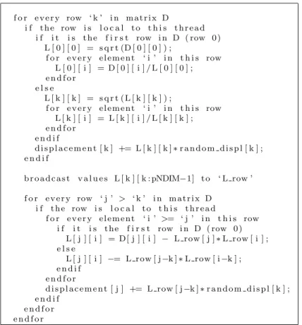
f o r e v e r y row ‘ k ’ i n m a tr i x D i f th e row i s l o c a l to t h i s t h r e a d i f i t i s th e f i r s t row i n D ( row 0 ) L [ 0 ] [ 0 ] = s q r t (D [ 0 ] [ 0 ] ) ; f o r e v e r y el em en t ‘ i ’ i n t h i s row L [ 0 ] [ i ] = D [ 0 ] [ i ] / L [ 0 ] [ 0 ] ; e n d f o r e l s e L [ k ] [ k ] = s q r t (L [ k ] [ k ] ) ; f o r e v e r y el em en t ‘ i ’ i n t h i s row L [ k ] [ i ] = L [ k ] [ i ] / L [ k ] [ k ] ; e n d f o r e n d i f d i s p l a c e m e n t [ k ] += L [ k ] [ k ]∗r a n d o m d i s p l [ k ] ; e n d i f b r o a d c a s t v a l u e s L [ k ] [ k : pNDIM−1] to ‘ L row ’ f o r e v e r y row ‘ j ’ > ‘ k ’ i n m a tr i x D i f th e row i s l o c a l to t h i s t h r e a d f o r e v e r y el em en t ‘ i ’ >= ‘ j ’ i n t h i s row i f i t i s th e f i r s t row i n D ( row 0 ) L [ j ] [ i ] = D[ j ] [ i ] − L row [ j ]∗L row [ i ] ; e l s e L [ j ] [ i ] −= L row [ j−k ]∗L row [ i−k ] ; e n d i f e n d f o r d i s p l a c e m e n t [ j ] += L row [ j−k ]∗r a n d o m d i s p l [ k ] ; e n d i f e n d f o r e n d f o r
Listing 1: Pseudocode for the computation of displacements with Cholesky decomposition
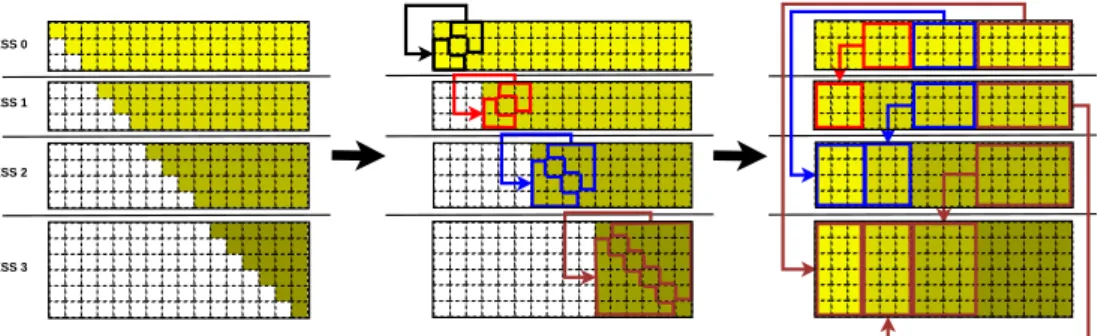
4.4.2. Fixman’s algorithm with balanced communications
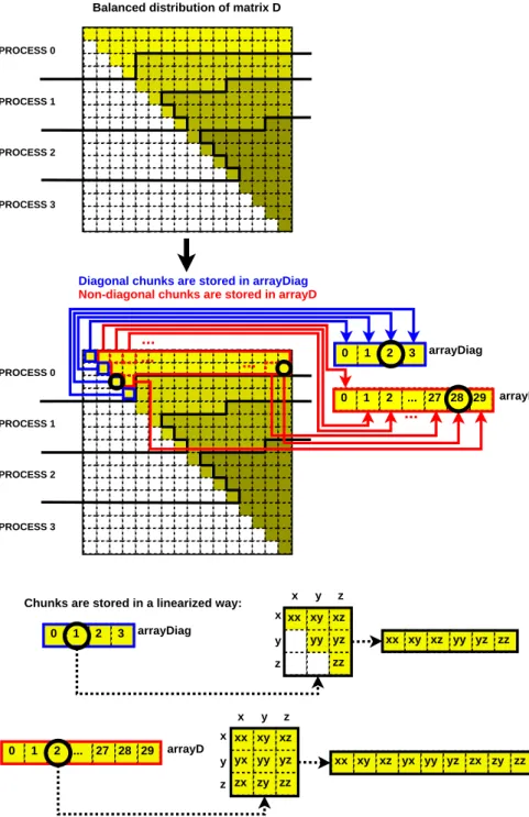
Figure 4 presents a domain decomposition and hence a workload distri-bution, both for MPI and UPC, focused on maximizing load balancing and exploiting local computations to reduce communications for Fixman’s
algo-rithm. Matrix D consists of diagonal and non-diagonal elements, and its
dis-tribution assigns to each process a balanced number of consecutive elements of each type, regardless of the particles to which they correspond. Thus, in Figure 4 the 16 diagonal elements are distributed among the 4 processes (each one receives 4 diagonal elements), and the 120 remaining elements are scattered (30 elements per process). Finally, every chunk is linearized in
arrayDiag (diagonal chunks) and arrayD (non-diagonal chunks) following the flattening process shown at the bottom of Figure 4. This distribution fa-vors local processing for diagonal values, as well as the balanced distribution of data and communications for non-diagonal values.
2 29 xx xy xz yx yy yz zx zy zz xx xy xz yx yy yz zx zy zz xx xy xz yy yz zz 0 1 ... 27 28 xx xy xz yy yz zz x y z x y z x y z x y z 0 1 2 3 arrayDiag arrayD 2 29 PROCESS 0 PROCESS 1 PROCESS 2 PROCESS 3 0 1 ... 27 28 0 1 2 3 arrayDiag arrayD ... ... ... ...
Diagonal chunks are stored in arrayDiag Non-diagonal chunks are stored in arrayD
Chunks are stored in a linearized way: PROCESS 0
PROCESS 1
PROCESS 2
PROCESS 3
Balanced distribution of matrix D
Figure 4: Balanced distribution of matrixDfor Fixman’s algorithm (detailed data struc-tures for process 0)
i n i t i a l i z e maximum e i g e n v a l u e ‘ eigmax ’ to 1 i n i t i a l i z e ‘ ei g en x ’ ( e i g e n v a l u e a p p r o x i m a t i o n s f o r each row ) to 1 w h i l e th e d e s i r e d a c c u r a c y f o r ‘ eigmax ’ i s not r e a c h e d i f th e i t e r a t i o n number i s even f o r e v e r y l o c a l el em en t i n ‘ arrayD ’ compute p a r t i a l a p p r o x i m a ti o n f o r ‘ eigmax ’ \ i n ‘ Dcopy ’ u s i n g ‘ ei g en x ’ e n d f o r f o r e v e r y l o c a l el em en t i n ‘ a r r a y D i a g ’ compute p a r t i a l a p p r o x i m a ti o n d i r e c t l y \ i n ‘ e i g e n x d ’ u s i n g ‘ ei g en x ’ e n d f o r a l l−to−a l l c o l l e c t i v e to g e t a l l p a r t i a l a p p r o x i m a t i o n s from ‘ Dcopy ’ f o r e v e r y l o c a l el em en t ‘ i ’ i n ‘ e i g e n x d ’ f o r e v e r y p r o c e s s ‘ j ’ sum th e p a r t i a l r e s u l t o f p r o c e s s ‘ j ’ i n ‘ Dcopy ’ \ to g e t th e f i n a l a p p r o x i m a ti o n o f ‘ e i g e n x d [ i ] ’ e n d f o r i f ‘ e i g e n x d [ i ] ’ i s th e maximum v a l u e update ‘ eigmax ’ e n d i f e n d f o r a l l g a t h e r th e computed v a l u e s i n ‘ e i g e n x d ’
a l l r e d u c e th e maximum v a l u e o f ‘ eigmax ’ from a l l p r o c e s s e s e l s e
th e same o p e r a t i o n s a s above , but ch a n g i n g ‘ ei g en x ’ \
by ‘ e i g e n x d ’ and v i c e v e r s a e n d i f
e n d w h i l e
Listing 2: Pseudocode for the parallel computation of the maximum eigenvalue with Fix-man’s algorithm
Listing 2 presents the pseudocode that implements the parallel
calcula-tion of the maximum eigenvalue in matrix D through an iterative method,
which can be analogously applied to the subsequent approximation of the
minimum eigenvalue and the elements of matrix S, as commented for the
se-quential code in Section 3. Each process calculates locally a partial result for the approximated eigenvalue using its assigned diffusion tensor values, and then an all-to-all collective communication is invoked by every process to get all the partial results of its assigned rows. Finally, each process computes the total approximation of its associated eigenvalues, an allgather collective operation is used to provide all processes with all the approximations, and an allreduce collective obtains the maximum eigenvalue of all processes in order to start a new iteration of the method. The computed eigenvalues are
here assigned alternatively to arrays eigenx and eigenx d with the goal of
com-mented in Section 3. As the distribution of particles is initially balanced, as well as the amount of communications performed by each process, there is no relevant workload difference among the processes, regardless of the number of iterations.
Besides load balancing, another benefit of this distribution is the opti-mized memory storage of variables, because it only considers the minimum number of elements that are necessary for the simulation instead of using the whole square matrix. Additionally, this implementation requires the use of indices that mark, for example, the starting position of the values asso-ciated to each particle in a dimension, which in turn increases slightly the complexity of the source code. However, these indices are computed only once before the simulation loop begins, and therefore they do not have a significant influence on performance.
4.4.3. Fixman’s algorithm with minimum communications
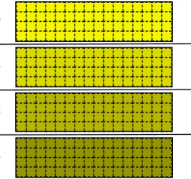
The previous algorithm for Fixman’s method has limited its scalability because of the overhead derived from the communications required at each iteration. In order to reduce the amount of communications, a block
dis-tribution of matrix D by rows is proposed in Figure 5, both for MPI and
UPC. This distribution considers that the particles in the system are evenly distributed between processes, and each of them computes all the diffusion tensor values of its associated particles. As a result, Fixman’s algorithm can be implemented using a minimum number of communications: the approx-imations of the correlation coefficients for every particle in every dimension are always computed locally by the corresponding process, and only an all-gather collective operation is necessary at the end of each iteration. The main drawback of this implementation is its higher computational cost, be-cause it has to compute roughly double the number of elements, as it does
not take full advantage of the symmetry in D (only locally). However, the
scalability of this approach is significantly higher than that of the previous algorithms: this is due to the reduced number of communications required, which allows to outperform previous approaches as the number of processes increases.
4.5. Implementation of communications using collective functions
As the previous subsections have shown, the most relevant communi-cations in the parallel simulations are collective operations, which involve
PROCESS 0
PROCESS 1
PROCESS 2
PROCESS 3
Figure 5: Work distribution withDas a full-size private matrix
multiple processes and perform common data movements and reduction op-erations (e.g., broadcast, all-to-all, allgather, allreduce...). Both MPI and UPC provide collective routines in their respective specifications (see [18] for UPC). However, UPC collectives generally present more limitations than MPI, which are derived from the strict management of the shared memory space in UPC. Many of these collective communications are performed using the same array as source and destination of the operation, which is supported
in MPI by the MPI IN PLACE wildcard, whereas UPC collectives do not
sup-port this feature, because data integrity would not be guaranteed. Moreover, the UPC collectives library presents additional issues, such as the necessary definition of source and destination as shared arrays (the most efficient UPC implementations are based on the use of the private memory space [16]) and the use of fixed-size data chunks for communications in all threads. These facts have traditionally led UPC programmers to replace these functions with raw data copy functions [16], reducing significantly the programmability of the applications.
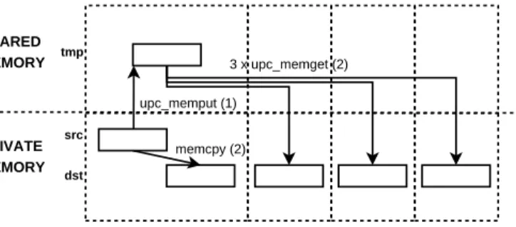
As a consequence of these limitations, the use of standard collective func-tions in the UPC code is not possible because many data transfers involve private arrays, a variable number of elements per thread or in-place com-munications. In order to address these issues, we have developed a library of extended UPC collectives [19]. Figure 6 presents an example of the data movements involved in an extended broadcast operation, which are UPC one-sided (that is, communications invoked by a single peer of the communi-cation) memory copy functions, where the source (src) and destination (dst) are both private arrays, using two steps: (1) the source thread copies the tar-get data to a temporary shared buffer (tmp), and (2) the rest of threads copy
the source data in parallel. This is a representative example of operation, shown for illustrative purposes, which is used in the library only for intra-node communications on shared memory, because it exploits the efficiency of the parallel access to shared memory [20]. For inter-node communications dif-ferent algorithms have been developed: (1) a binomial tree approach for data movement collectives, and (2) a specific concatenation-like procedure [21] for the in-place all-to-all collective, which avoids source data overwriting and balances the workload among threads by calculating the minimum neces-sary data transfers according to the number of threads in the program. As a result, these functions provide an efficient implementation of the desired communications in UPC.
SHARED MEMORY
PRIVATE MEMORY
THREAD 0 THREAD 1 THREAD 2 THREAD 3
src dst tmp upc_memput (1) 3 x upc_memget (2) memcpy (2)
Figure 6: Data movements in a UPC broadcast implementation based on private arrays
5. Performance evaluation
The evaluation of the developed parallel Brownian dynamics codes has
been accomplished on the JuRoPa supercomputer at J¨ulich Supercomputing
Centre, ranked 63rd in the TOP500 List of June 2012. It is a representative supercomputer system with hybrid shared/distributed memory architecture which consists of 2208 compute nodes, each of them including 2 Intel Xeon X5570 (Nehalem-EP) quad-core processors at 2.93 GHz (hence 8 cores per node), 24 GB of DDR3 memory at 1066 MHz and InfiniBand QDR HCA with non-blocking Fat Tree topology. The UPC compiler used was Berkeley UPC v2.14.2 (a UPC-to-C source-to-source compiler, released in May 2012) with the Intel C Compiler v11.1 as backend C compiler, and relying on the IBV (InfiniBand Verbs) conduit for efficient communications on InfiniBand. The MPI compiler used here is ParaStation MPI 5.0.27-1 (March 2012) [22]. All the MPI and UPC executions were compiled with the optimization flag
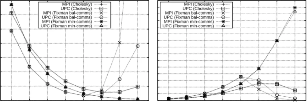
-O3. In order to perform a fair comparison, all speedup results have been calculated taking the execution times of the original sequential C code as baseline, as it represents the fastest approach. The problem size considered for each graph (Figures 7-9) is fixed for a varying number of cores, thus showing strong scaling, and all tests use a fill-up policy for process scheduling in the nodes of the testbed system, always with one process per physical core. Three different versions of the simulations are shown depending on the algorithm and work distribution used for the computation of random displacements: (1) using Cholesky decomposition (see Section 4.4.1), (2) using Fixman’s algorithm with the distribution presented in Section 4.4.2
that balances workload and communications (referred to as bal-comms from
now on), and (3) using Fixman’s algorithm with matrix D distributed to
minimize communications, as described in Section 4.4.3 (referred to as
min-comms).
Figure 7 shows the execution times and speedups of the parallel simulation of 256 particles over 100 time steps (double the workload of Table 1). The results show that, on the one hand, the best performance up to 16 cores is obtained by the version that uses Fixman with balanced workload and
optimized storage (bal-comms), with very similar results for MPI and UPC.
However, the weight of allgather and all-to-all communications in covar()
limits heavily the scalability with this approach from 32 cores onward, as the ratio computation/communication time is lower than in the other tests.
On the other hand, Fixman min-comms presents the opposite situation: the
redundant computations cause poor performance for a small number of cores, but the minimization of communications provides good scalability as the number of cores increases, even for 128 cores (that is, when only 2 particles per core are processed). The codes based on Cholesky are able to scale up to 32 cores, but performance decreases for 64 and 128 cores because of the significant weight of the communication overhead in the total execution time. These results also show that codes relying on Fixman’s algorithm outperform
Cholesky-based codes, either using the bal-comms version (except for a large
number of cores) or the min-comms one. Additionally, the execution times
when using Cholesky show a higher increase with the number of particles than in the codes based on Fixman (see Table 1), confirming that Fixman is the best choice for the generation of random displacements, hence discarding the use of Cholesky with larger problem sizes.
Comparing MPI and UPCbal-comms codes when using 32 or more cores,
0 5 10 15 20 25 30 35 1 2 4 8 16 32 64 128 Execution Time (s) Number of Cores
MPI & UPC Brownian Dynamics, N = 256
MPI (Cholesky) UPC (Cholesky) MPI (Fixman bal-comms) UPC (Fixman bal-comms) MPI (Fixman min-comms) UPC (Fixman min-comms)
1 2 4 8 16 32 64 128 0 4 8 12 16 20 24 28 32 36 40 44 48 52 56 60 Speedup Number of Cores
MPI & UPC Brownian Dynamics, N = 256
MPI (Cholesky) UPC (Cholesky) MPI (Fixman bal-comms) UPC (Fixman bal-comms) MPI (Fixman min-comms) UPC (Fixman min-comms)
Figure 7: Performance results with 256 particles
0 25 50 75 100 125 150 175 200 225 250 275 300 325 350 375 400 425 450 1 2 4 8 16 32 64 128 256 512 Execution Time (s) Number of Cores
MPI & UPC Brownian Dynamics, N = 1024
MPI (Fixman bal-comms) UPC (Fixman bal-comms) MPI (Fixman min-comms) UPC (Fixman min-comms)
1 2 4 8 16 32 64 128 256 512 0 32 64 96 128 160 192 224 Speedup Number of Cores
MPI & UPC Brownian Dynamics, N = 1024
MPI (Fixman bal-comms) UPC (Fixman bal-comms) MPI (Fixman min-comms) UPC (Fixman min-comms)
Figure 8: Performance results with 1024 particles
0 500 1000 1500 2000 2500 3000 3500 4000 4500 5000 5500 6000 6500 7000 7500 8000 8500 1 2 4 8 16 32 64 128 256 512 1024 2048 Execution Time (s) Number of Cores
MPI & UPC Brownian Dynamics, N = 4096
MPI (Fixman bal-comms) UPC (Fixman bal-comms) MPI (Fixman min-comms) UPC (Fixman min-comms)
1 2 4 8 16 32 64 128 256 512 1024 2048 0 64 128 192 256 320 384 448 512 576 640 704 768 832 Speedup Number of Cores
MPI & UPC Brownian Dynamics, N = 4096
MPI (Fixman bal-comms) UPC (Fixman bal-comms) MPI (Fixman min-comms) UPC (Fixman min-comms)
due both to memory requirements for internal buffering and synchronization costs, becomes an important performance bottleneck, in particular for MPI. Regarding UPC, our implementation of the extended all-to-all function (see Section 4.5) manages memory and synchronizations more efficiently.
Figures 8 and 9 present the performance results with 50 time steps using 1024 and 4096 particles, respectively. In general, the results of the simula-tions are very similar to those of Figure 7, so an analogous interpretation
can also be applied here: on the one hand, the bal-comms version obtains
an almost linear speedup up to 32 cores for 1024 particles, and up to 64
cores for 4096 particles. Additionally, bal-comms obtains the best results up
to the number of cores for which the computation time is still higher than the communication time (i.e., up to 32 cores for 1024 particles, and up to 64 cores with MPI and 128 cores with UPC for 4096 particles), and again UPC all-to-all communications represent a better choice than MPI in the
simulation. On the other hand, min-comms shows the highest scalability,
both for MPI and UPC, achieving in general a speedup of about half of the number of cores being used (i.e., a parallel efficiency of around 50%). Taking into account that this implementation requires almost double the number of computations of the original sequential code (hence its speedup with one core is around 0.6), this represents a significant scalability. Furthermore, the
min-comms results in Figure 9 show a slight difference between MPI and UPC for 1024 and 2048 cores, mainly caused by the shared memory cache coherence mechanisms of the UPC runtime, whose implementation presents a significant overhead when handling thousands of cores.
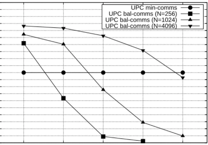
Another factor to be considered is the number of particles handled per core, which limits the exploitation of each parallel solution. For example, according to the UPC performance results of Figures 7-9 and assuming that
all time steps in a simulation have the same workload, thebal-comms version
generally obtains the best results when 16 or more particles per core are simulated in a system with 256 particles (that is, when 16 or less cores are
used); for simulations of 1024 and 4096 particles, bal-comms obtains the best
results with 32 or more particles per core. This situation is illustrated in
Figure 10 in the range of 16–256 cores, where the efficiency of thebal-comms
algorithm for all problem sizes can be seen in relative terms compared to
the performance of the min-comms counterpart: the higher the percentage
is, the more efficient the algorithm is for the corresponding problem size.
These results indicate that the bal-comms approach is overall a good choice
memory is limited (because of the optimized storage of matrix D commented in Section 4.4.2) and the ratio computation/communication time is high, regardless of the actual number of cores or particles used in the simulation.
0 10 20 30 40 50 60 70 80 90 100 110 120 130 140 150 160 170 180 190 200 16 32 64 128 256 Relative Efficiency (%) Number of Cores
UPC Brownian Dynamics - Algorithm Efficiency UPC min-comms UPC bal-comms (N=256) UPC bal-comms (N=1024) UPC bal-comms (N=4096)
Figure 10: Efficiency comparison between bal-comms and min-comms algorithms, ex-pressed as the percentage of the efficiency of themin-comms code
6. Conclusions
The simulation of Brownian dynamics is a very relevant tool to analyze the interaction of particles under certain conditions, representing a computa-tionally intensive task that has motivated the implementation of an efficient and scalable parallel code to support the study of large particle systems on high performance supercomputers under representative constraints. Thus, this work has presented the design and implementation of a parallel Brownian dynamics simulation using the MPI library and the PGAS UPC language. While MPI represents a traditional and widely extended message-passing parallel programming approach on distributed memory, UPC focuses on pro-viding programmability resources for high performance applications by using the PGAS memory model, which is especially suitable on hybrid shared/dis-tributed memory architectures.
The main contributions of this work are: (1) the analysis of data depen-dencies in the simulation codes and the proposed domain decompositions for
parallel systems, (2) the assessment of the alternatives in the work distribu-tions in order to maximize performance and manage memory requirements efficiently, (3) the application of more efficient and usable collective commu-nications for UPC, and (4) the performance evaluation of different versions of the parallel code on a representative supercomputer with a large number of cores.
The experimental results have shown that codes using Fixman’s algorithm outperform codes with Cholesky decomposition, and that there is no single optimal approach for all scenarios: the balanced communications version (bal-comms) presents the best performance when computation time is higher
than communication time, whereas a more scalable approach (min-comms)
can take advantage of higher numbers of cores. Thus, the implemented ap-proaches, both with MPI and UPC, are able to scale performance up to
thou-sands of cores (min-comms) while providing an alternative implementation
with less memory requirements for a reduced number of cores (bal-comms).
Regarding the programming models considered, significant differences have been found. On the one hand, the higher maturity of MPI routines has pro-vided high performance and stability (showing the best performance when using more than 1024 cores) at the cost of a higher programming effort. On the other hand, UPC has provided lower time to solution, allowing the de-velopment of quick parallel prototypes thanks to its shared memory view while providing good scalability by taking advantage of the use of one-sided operations on a hybrid shared/distributed memory architecture, such as the evaluated supercomputer (a cluster of multicore processors). Moreover, its limitations in the support of collective operations have been overcome, thus being UPC able to rival MPI in performance and even to outperform its MPI
bal-comms counterpart code when an extensive use of collective communi-cations (mainly in-place ones) is necessary, showing better results in this scenario as the number of cores increases.
As main outcome of this work, developers and users of parallel simulation codes in general, and of Brownian dynamics in particular, would significantly benefit from the lessons learned during the development of the multiple par-allel implementations presented in this paper.
Acknowledgments
This work was funded by the Ministry of Science and Innovation of Spain (Project TIN2010-16735) and by the Galician Government (Pre-doctoral
Pro-gram “Mar´ıa Barbeito” and ProPro-gram for the Consolidation of Competitive
Research Groups, ref. 2010/6). We gratefully thank the J¨ulich
Supercom-puting Centre for providing access to the JuRoPa supercomputer.
Appendix A. Rotne-Prager tensor
In this Appendix the expression for the regularized version of the Rotne-Prager tensor in periodic boundary conditions is given. The expression fol-lows closely the one derived by Beenaker [23] with the extension of the reg-ularization for distances r <2a.
The tensor D is split into four parts:
D(rij) = X ℓℓℓ θ(rij(0)−2a) [D(1)(rij(ℓ)) +D(2)(rij(ℓ)) +D(3)(rij(ℓ))] +(1−θ(rij(0)−2a))D(4)(rij(ℓ)) (A.1) where θ(x) = 0 : x <0 1 : x≥0 (A.2)
is the step function andrij(ℓ)=ri−rj+ℓℓℓL, withLthe simulation box length and ℓℓℓ= (ℓx, ℓy, ℓz)T ∈Z3, i.e. the resulting tensor contains all contributions between particle iandj plus all periodic images of particlej. The individual terms of the tensor are given by:
D(1)(rij) = kBT 6πηa 1− √6 πκa 1 + 20 9 κ 2a2 Iδijδαβ (A.3a) D(2)(rij) = kBT 6πηaθ(rij −Rc,D) ( I 3 4 a rij +1 2 a3 r3 ij erfc(κrij) (A.3b) +I√1 π 4κ7a3r4ij+ 3κ3arij2 −20κ5a3rij2 − 9 2κa+ 14κ 3a3+κa3 r2 ij ×exp(−κ2r2 ij) + ˆrˆr 3 4 a rij − 3 2 a3 r3 ij erfc(κrij) −ˆrˆr 4κ7a3r4ij + 3κ3arij2 −16κ5a3rij2 − 3 2κa+ 2κ 3a3 + 3κa3 r2 ij ×exp (−κ 2r2 ij) √ π )
D(3)(rij) = kBT 6πηa 1 V X |k|<kmax (I−ˆkˆk) a−1 3a 3k2 1 + 1 4 k2 κ2 + 1 8 k4 κ4 6π k2 ×exp 1 4 k2 κ2 cos(krij(ℓ)) (A.3c) D(4)(rij) = kBT 6πηa 1− 9 32 rij a I+ X ℓ rij(ℓ)>2a D(2)(rij(ℓ)) +D(3)(rij(ℓ)) (A.3d) with δij = 0 : i6=j 1 : i=j (A.4)
the Kronecker-δ and α, β = x, y, z being cartesian indices of the position
vectors. Since these expressions are approximations to the evaluation of an infinite sum, parameters which control the limits in the sums are introduced, i.e. Eq. A.3b is evaluated only for particle pairs within a cutoff radius Rc,D and Eq. A.3c is limited to wavenumbers |k|< kmax, where k= 2π/Ln, n∈ Z3. The parametersRc,D, kmax, κof the periodic version of the Rotne-Prager
tensor have to be determined according to an error threshold ǫ. There is no
unique set of parameters fulfilling this requirement, but one may obtain an
optimal set of parameters which, for a given ǫ, minimizes the runtime.
References
[1] Y. Zhang, J.J. de Pablo, M.D. Graham, J. Chem. Phys. 136 (2012) 014901
[2] G.A. Huber, J.A. McCammon, Comput. Phys. Commun. 181 (2010) 1896
[3] J. Garc´ıa de la Torre, J.G. Hern´andez Cifre, A. Ortega, R.R. Schmidt, M.X. Fernandes, H.E. P´erez S´anchez, R. Pamies, J. Chem. Theory Com-put. 5 (2009) 2606
[4] L. Dematte, IEEE/ACM Trans. Comput. Biol. Bioinf. 9 (2012) 655
[5] M. D lugosz, P. Zieli´nski, J. Trylska, J. Comput. Chem. 32 (2011) 2734
[7] J. Rotne, S. Prager, J. Chem. Phys. 50 (1969) 4831
[8] A. Satoh, Introduction to Molecular-Microsimulation for Colloidal Dis-persions (Elsevier, Amsterdam, 2003)
[9] M. Fixman, Macromolecules 19 (1986) 1204
[10] M.P. Allen, D.J. Tildesley, Computer Simulation of Liquids (Oxford Science Publications, Oxford, 1987)
[11] E.F. Carter, Forth Dimensions 16 (1994) 24
[12] C. Canuto, M.Y. Hussaini, A. Quarteroni, Spectral Methods in Fluid Dynamics (Springer, Berlin, 1988)
[13] T. Schlick, D.A. Beard, J. Huang, D. Strahs, X. Qian, Comp. Sci. Eng. 2 (2000) 38
[14] R.M. Jendrejack, M.D. Graham, J.J. de Pablo, J. Chem. Phys. 113 (2000) 2894
[15] T. El-Ghazawi, W. Carlson, T. Sterling, K. Yelick, UPC: Distributed Shared Memory Programming (John Wiley & Sons, New Jersey, 2005) [16] T. El-Ghazawi, S. Chauvin, UPC Benchmarking Issues, in: Proc. 30th
Int. Conf. on Parallel Process. (2001) 365
[17] R. Murty, D. Okunbor, Parallel Comput. 25 (1999) 217
[18] UPC Consortium, UPC Collective Operations Specifications v1.0 (2003) http://upc.gwu.edu/docs/UPC Coll Spec V1.0.pdf (accessed Dec. 2012)
[19] C. Teijeiro, G.L. Taboada, J. Touri˜no, R. Doallo, J.C. Mouri˜no, D.A.
Mall´on, B. Wibecan, J. Comput. Sci. Technol. 28 (2013) (to appear)
[20] G.L. Taboada, C. Teijeiro, J. Touri˜no, B.B. Fraguela, R. Doallo, J.C.
Mouri˜no, D.A. Mall´on, A. G´omez, Performance Evaluation of Unified
Parallel C Collective Communications, in: Proc. 11th IEEE Int. Conf. on High Perform. Comput. and Commun. (2009) 69
[21] J. Bruck, C.-T. Ho, S. Kipnis, E. Upfal, D. Weathersby, IEEE Trans. Parallel Distrib. Syst. 8 (1997) 1143
[22] ParTec, ParaStation MPI (2012) http://www.par-tec.com/products/ parastation-mpi.html (accessed Dec. 2012)