10
Techniques of Integration
10.1 Powers of sine and osine
Functions consisting of products of the sine and cosine can be integrated by using substi-tution and trigonometric identities. These can sometimes be tedious, but the technique is straightforward. Some examples will suffice to explain the approach.
EXAMPLE 10.1.1 Evaluate Z
sin5x dx. Rewrite the function: Z sin5x dx= Z sinxsin4x dx= Z sinx(sin2x)2dx= Z sinx(1−cos2x)2dx. Now useu = cosx, du=−sinx dx:
Z sinx(1−cos2x)2dx= Z −(1−u2)2du = Z −(1−2u2+u4)du =−u+ 2 3u 3− 1 5u 5+C =−cosx+ 2 3cos 3x− 1 5cos 5x+C. 203
EXAMPLE 10.1.2 Evaluate Z
sin6x dx. Use sin2x = (1−cos(2x))/2 to rewrite the function: Z sin6x dx= Z (sin2x)3dx= Z (1 −cos 2x)3 8 dx = 1 8 Z
1−3 cos 2x+ 3 cos22x−cos32x dx. Now we have four integrals to evaluate:
Z 1dx=x and Z −3 cos 2x dx=−3 2sin 2x are easy. The cos32x integral is like the previous example:
Z −cos32x dx= Z −cos 2xcos22x dx = Z −cos 2x(1−sin22x)dx = Z −12(1−u2)du =−1 2 u− u 3 3 =−1 2 sin 2x− sin 32x 3 .
And finally we use another trigonometric identity, cos2x= (1 + cos(2x))/2: Z 3 cos22x dx= 3 Z 1 + cos 4x 2 dx= 3 2 x+ sin 4x 4 . So at long last we get
Z sin6x dx= x 8 − 3 16sin 2x− 1 16 sin 2x− sin 32x 3 + 3 16 x+ sin 4x 4 +C. EXAMPLE 10.1.3 Evaluate Z
sin2xcos2x dx. Use the formulas sin2x= (1−cos(2x))/2 and cos2x = (1 + cos(2x))/2 to get:
Z sin2xcos2x dx= Z 1 −cos(2x) 2 · 1 + cos(2x) 2 dx.
10.2 Trigonometric Substitutions 205
Exercises 10.1.
Find the antiderivatives.
1. Z sin2x dx ⇒ 2. Z sin3x dx ⇒ 3. Z sin4x dx ⇒ 4. Z cos2xsin3x dx ⇒ 5. Z cos3x dx ⇒ 6. Z sin2xcos2x dx ⇒ 7. Z cos3xsin2x dx ⇒ 8. Z sinx(cosx)3/2dx ⇒ 9. Z sec2xcsc2x dx ⇒ 10. Z tan3xsecx dx ⇒ 10.2 Trigonometri Substitutions
So far we have seen that it sometimes helps to replace a subexpression of a function by a single variable. Occasionally it can help to replace the original variable by something more complicated. This seems like a “reverse” substitution, but it is really no different in principle than ordinary substitution.
EXAMPLE 10.2.1 Evaluate Z
p
1−x2dx. Let x = sinu so dx= cosu du. Then Z p 1−x2dx= Z p 1−sin2ucosu du= Z √
cos2ucosu du.
We would like to replace √cos2u by cosu, but this is valid only if cosu is positive, since
√
cos2uis positive. Consider again the substitution x= sinu. We could just as well think of this asu= arcsinx. If we do, then by the definition of the arcsine, −π/2≤u≤π/2, so cosu≥0. Then we continue:
Z √ cos2ucosu du= Z cos2u du= Z 1 + cos 2u 2 du= u 2 + sin 2u 4 +C = arcsinx 2 + sin(2 arcsinx) 4 +C.
This is a perfectly good answer, though the term sin(2 arcsinx) is a bit unpleasant. It is possible to simplify this. Using the identity sin 2x = 2 sinxcosx, we can write sin 2u = 2 sinucosu= 2 sin(arcsinx)p1−sin2u = 2x
q
1−sin2(arcsinx) = 2xp1−x2. Then the full antiderivative is arcsinx 2 + 2x√1−x2 4 = arcsinx 2 + x√1−x2 2 +C.
This type of substitution is usually indicated when the function you wish to integrate contains a polynomial expression that might allow you to use the fundamental identity sin2x+ cos2x= 1 in one of three forms:
cos2x= 1−sin2x sec2x = 1 + tan2x tan2x = sec2x−1.
If your function contains 1−x2, as in the example above, tryx = sinu; if it contains 1 +x2 try x = tanu; and if it contains x2 −1, try x = secu. Sometimes you will need to try something a bit different to handle constants other than one.
EXAMPLE 10.2.2 Evaluate Z
p
4−9x2dx. We start by rewriting this so that it looks more like the previous example:
Z p 4−9x2dx= Z p 4(1−(3x/2)2)dx= Z 2p1−(3x/2)2dx. Now let 3x/2 = sinu so (3/2)dx= cosu du or dx= (2/3) cosu du. Then
Z 2p1−(3x/2)2dx= Z 2p1−sin2u(2/3) cosu du= 4 3 Z cos2u du = 4u 6 + 4 sin 2u 12 +C = 2 arcsin(3x/2) 3 + 2 sinucosu 3 +C = 2 arcsin(3x/2) 3 + 2 sin(arcsin(3x/2)) cos(arcsin(3x/2)) 3 +C = 2 arcsin(3x/2) 3 + 2(3x/2)p 1−(3x/2)2 3 +C = 2 arcsin(3x/2) 3 + x√4−9x2 2 +C,
using some of the work from example 10.2.1. EXAMPLE 10.2.3 Evaluate
Z p
1 +x2dx. Let x= tanu, dx= sec2u du, so Z
p
1 +x2dx= Z
p
1 + tan2usec2u du=Z √sec2usec2u du. Since u= arctan(x),−π/2≤u≤π/2 and secu≥0, so √sec2u= secu. Then
Z √
sec2usec2u du=Z sec3u du. In problems of this type, two integrals come up frequently:
Z
sec3u du and R
secu du. Both have relatively nice expressions but they are a bit tricky to discover.
10.2 Trigonometric Substitutions 207
First we do R
secu du, which we will need to compute Z
sec3u du: Z
secu du= Z
secusecu+ tanu secu+ tanu du =
Z
sec2u+ secutanu secu+ tanu du.
Now let w = secu + tanu, dw = secutanu+ sec2u du, exactly the numerator of the function we are integrating. Thus
Z
secu du= Z
sec2u+ secutanu secu+ tanu du= Z 1 wdw = ln|w|+C = ln|secu+ tanu|+C. Now for Z sec3u du: sec3u = sec 3u 2 + sec3u 2 = sec3u 2 + (tan2u+ 1) secu 2 = sec 3u 2 + secutan2u 2 + secu 2 =
sec3u+ secutan2u
2 +
secu 2 .
We already know how to integrate secu, so we just need the first quotient. This is “simply” a matter of recognizing the product rule in action:
Z
sec3u+ secutan2u du= secutanu. So putting these together we get
Z
sec3u du= secutanu
2 +
ln|secu+ tanu|
2 +C,
and reverting to the original variablex: Z p 1 +x2dx= secutanu 2 + ln|secu+ tanu| 2 +C = sec(arctanx) tan(arctanx) 2 + ln|sec(arctanx) + tan(arctanx)| 2 +C = x √ 1 +x2 2 + ln|√1 +x2+x| 2 +C,
using tan(arctanx) =x and sec(arctanx) = q
Exercises 10.2.
Find the antiderivatives.
1. Z cscx dx⇒ 2. Z csc3x dx ⇒ 3. Z p x2 −1dx ⇒ 4. Z p 9 + 4x2dx ⇒ 5. Z xp1−x2dx ⇒ 6. Z x2p1−x2dx ⇒ 7. Z 1 √ 1 +x2 dx⇒ 8. Z p x2+ 2x dx ⇒ 9. Z 1 x2(1 +x2)dx⇒ 10. Z x2 √ 4−x2 dx⇒ 11. Z √ x √ 1−x dx⇒ 12. Z x3 √ 4x2 −1 dx ⇒ 10.3 Integration by Parts
We have already seen that recognizing the product rule can be useful, when we noticed that
Z
sec3u+ secutan2u du= secutanu.
As with substitution, we do not have to rely on insight or cleverness to discover such antiderivatives; there is a technique that will often help to uncover the product rule.
Start with the product rule: d
dxf(x)g(x) = f
′(x)g(x) +f(x)g′(x).
We can rewrite this as
f(x)g(x) = Z f′(x)g(x)dx+ Z f(x)g′(x)dx, and then Z f(x)g′(x)dx=f(x)g(x)− Z f′(x)g(x)dx.
This may not seem particularly useful at first glance, but it turns out that in many cases we have an integral of the form
Z
f(x)g′(x)dx
but that
Z
f′(x)g(x)dx
is easier. This technique for turning one integral into another is called integration by parts, and is usually written in more compact form. If we letu =f(x) andv =g(x) then
10.3 Integration by Parts 209 du=f′(x)dx anddv =g′(x)dxand Z u dv =uv− Z v du.
To use this technique we need to identify likely candidates foru =f(x) anddv =g′(x)dx.
EXAMPLE 10.3.1 Evaluate Z
xlnx dx. Let u = lnx so du= 1/x dx. Then we must let dv=x dx so v=x2/2 and Z xlnx dx= x 2lnx 2 − Z x2 2 1 x dx= x2lnx 2 − Z x 2dx= x2lnx 2 − x2 4 +C. EXAMPLE 10.3.2 Evaluate Z
xsinx dx. Let u = x so du = dx. Then we must let dv= sinx dx so v=−cosx and
Z
xsinx dx=−xcosx− Z
−cosx dx=−xcosx+ Z
cosx dx=−xcosx+ sinx+C.
EXAMPLE 10.3.3 Evaluate Z
sec3x dx. Of course we already know the answer to this, but we needed to be clever to discover it. Here we’ll use the new technique to discover the antiderivative. Let u = secx and dv = sec2x dx. Then du= secxtanx dx and v = tanx and
Z
sec3x dx= secxtanx− Z tan2xsecx dx = secxtanx− Z (sec2x−1) secx dx = secxtanx− Z sec3x dx+ Z secx dx.
At first this looks useless—we’re right back to Z
sec3x dx. But looking more closely: Z
sec3x dx= secxtanx− Z sec3x dx+ Z secx dx Z sec3x dx+ Z
sec3x dx= secxtanx+ Z
secx dx 2
Z
sec3x dx= secxtanx+ Z
secx dx Z
sec3x dx= secxtanx
2 + 1 2 Z secx dx = secxtanx 2 + ln|secx+ tanx| 2 +C. EXAMPLE 10.3.4 Evaluate Z
x2sinx dx. Let u=x2, dv= sinx dx; then du= 2x dx and v = −cosx. Now
Z
x2sinx dx = −x2cosx+ Z
2xcosx dx. This is better than the original integral, but we need to do integration by parts again. Let u= 2x, dv = cosx dx; then du= 2 and v= sinx, and
Z x2sinx dx=−x2cosx+ Z 2xcosx dx =−x2cosx+ 2xsinx− Z 2 sinx dx =−x2cosx+ 2xsinx+ 2 cosx+C.
Such repeated use of integration by parts is fairly common, but it can be a bit tedious to accomplish, and it is easy to make errors, especially sign errors involving the subtraction in the formula. There is a nice tabular method to accomplish the calculation that minimizes the chance for error and speeds up the whole process. We illustrate with the previous example. Here is the table:
sign u dv x2 sinx − 2x −cosx 2 −sinx − 0 cosx or u dv x2 sinx −2x −cosx 2 −sinx 0 cosx
10.3 Integration by Parts 211 To form the first table, we start withuat the top of the second column and repeatedly compute the derivative; starting with dv at the top of the third column, we repeatedly compute the antiderivative. In the first column, we place a “−” in every second row. To form the second table we combine the first and second columns by ignoring the boundary; if you do this by hand, you may simply start with two columns and add a “−” to every second row.
To compute with this second table we begin at the top. Multiply the first entry in columnu by the second entry in column dv to get −x2cosx, and add this to the integral of the product of the second entry in columnuand second entry in columndv. This gives:
−x2cosx+ Z
2xcosx dx,
or exactly the result of the first application of integration by parts. Since this integral is not yet easy, we return to the table. Now we multiply twice on the diagonal, (x2)(−cosx) and (−2x)(−sinx) and then once straight across, (2)(−sinx), and combine these as
−x2cosx+ 2xsinx− Z
2 sinx dx,
giving the same result as the second application of integration by parts. While this integral is easy, we may return yet once more to the table. Now multiply three times on the diagonal to get (x2)(−cosx), (−2x)(−sinx), and (2)(cosx), and once straight across, (0)(cosx). We combine these as before to get
−x2cosx+ 2xsinx+ 2 cosx+ Z
0dx=−x2cosx+ 2xsinx+ 2 cosx+C.
Typically we would fill in the table one line at a time, until the “straight across” multipli-cation gives an easy integral. If we can see that theu column will eventually become zero, we can instead fill in the whole table; computing the products as indicated will then give the entire integral, including the “+C”, as above.
Exercises 10.3.
Find the antiderivatives.
1. Z xcosx dx ⇒ 2. Z x2cosx dx ⇒ 3. Z xexdx ⇒ 4. Z xex2dx ⇒ 5. Z sin2x dx ⇒ 6. Z lnx dx ⇒
7. Z xarctanx dx⇒ 8. Z x3sinx dx ⇒ 9. Z x3cosx dx ⇒ 10. Z xsin2x dx ⇒ 11. Z xsinxcosx dx ⇒ 12. Z arctan(√x)dx⇒ 13. Z sin(√x)dx⇒ 14. Z sec2xcsc2x dx ⇒ 10.4 Rational Funtions
A rational function is a fraction with polynomials in the numerator and denominator. For example, x3 x2+x−6, 1 (x−3)2, x2+ 1 x2−1,
are all rational functions of x. There is a general technique called “partial fractions” that, in principle, allows us to integrate any rational function. The algebraic steps in the technique are rather cumbersome if the polynomial in the denominator has degree more than 2, and the technique requires that we factor the denominator, something that is not always possible. However, in practice one does not often run across rational functions with high degree polynomials in the denominator for which one has to find the antiderivative function. So we shall explain how to find the antiderivative of a rational function only when the denominator is a quadratic polynomial ax2+bx+c.
We should mention a special type of rational function that we already know how to integrate: If the denominator has the form (ax+b)n, the substitution u = ax+b will always work. The denominator becomes un, and each x in the numerator is replaced by (u −b)/a, and dx = du/a. While it may be tedious to complete the integration if the numerator has high degree, it is merely a matter of algebra.
10.4 Rational Functions 213
EXAMPLE 10.4.1 Find
Z x3
(3−2x)5 dx. Using the substitution u= 3−2x we get
Z x3 (3−2x)5 dx= 1 −2 Z u−3 −2 3 u5 du= 1 16 Z u3−9u2 + 27u−27 u5 du = 1 16 Z u−2−9u−3+ 27u−4−27u−5du = 1 16 u−1 −1 − 9u−2 −2 + 27u−3 −3 − 27u−4 −4 +C = 1 16 (3−2x)−1 −1 − 9(3−2x)−2 −2 + 27(3−2x)−3 −3 − 27(3−2x)−4 −4 +C =− 1 16(3−2x) + 9 32(3−2x)2 − 9 16(3−2x)3 + 27 64(3−2x)4 +C
We now proceed to the case in which the denominator is a quadratic polynomial. We can always factor out the coefficient ofx2 and put it outside the integral, so we can assume that the denominator has the formx2+bx+c. There are three possible cases, depending on how the quadratic factors: either x2+bx+c= (x−r)(x−s), x2+bx+c= (x−r)2, or it doesn’t factor. We can use the quadratic formula to decide which of these we have, and to factor the quadratic if it is possible.
EXAMPLE 10.4.2 Determine whether x2+x+ 1 factors, and factor it if possible. The quadratic formula tells us thatx2+x+ 1 = 0 when
x= −1±
√
1−4
2 .
Since there is no square root of −3, this quadratic does not factor.
EXAMPLE 10.4.3 Determine whether x2−x−1 factors, and factor it if possible. The quadratic formula tells us thatx2−x−1 = 0 when
x= 1± √ 1 + 4 2 = 1±√5 2 . Therefore x2−x−1 = x− 1 + √ 5 2 ! x− 1− √ 5 2 ! .
Ifx2+bx+c= (x−r)2 then we have the special case we have already seen, that can be handled with a substitution. The other two cases require different approaches.
If x2+bx+c= (x−r)(x−s), we have an integral of the form Z
p(x)
(x−r)(x−s)dx
where p(x) is a polynomial. The first step is to make sure that p(x) has degree less than 2.
EXAMPLE 10.4.4 Rewrite Z
x3
(x−2)(x+ 3)dxin terms of an integral with a numer-ator that has degree less than 2. To do this we use long division of polynomials to discover that x3 (x−2)(x+ 3) = x3 x2+x−6 =x−1 + 7x−6 x2+x−6 =x−1 + 7x−6 (x−2)(x+ 3), so Z x3 (x−2)(x+ 3)dx= Z x−1dx+ Z 7x−6 (x−2)(x+ 3)dx. The first integral is easy, so only the second requires some work.
Now consider the following simple algebra of fractions: A x−r + B x−s = A(x−s) +B(x−r) (x−r)(x−s) = (A+B)x−As−Br (x−r)(x−s) .
That is, adding two fractions with constant numerator and denominators (x−r) and (x−s) produces a fraction with denominator (x−r)(x−s) and a polynomial of degree less than 2 for the numerator. We want to reverse this process: starting with a single fraction, we want to write it as a sum of two simpler fractions. An example should make it clear how to proceed. EXAMPLE 10.4.5 Evaluate Z x3 (x−2)(x+ 3)dx. We start by writing 7x−6 (x−2)(x+ 3) as the sum of two fractions. We want to end up with
7x−6 (x−2)(x+ 3) = A x−2 + B x+ 3. If we go ahead and add the fractions on the right hand side we get
7x−6
(x−2)(x+ 3) =
(A+B)x+ 3A−2B (x−2)(x+ 3) .
So all we need to do is find A and B so that 7x−6 = (A+B)x+ 3A−2B, which is to say, we need 7 =A+B and −6 = 3A−2B. This is a problem you’ve seen before: solve a
10.4 Rational Functions 215 system of two equations in two unknowns. There are many ways to proceed; here’s one: If 7 =A+BthenB= 7−Aand so−6 = 3A−2B = 3A−2(7−A) = 3A−14+2A= 5A−14. This is easy to solve forA: A= 8/5, and then B= 7−A= 7−8/5 = 27/5. Thus
Z 7x −6 (x−2)(x+ 3) dx= Z 8 5 1 x−2 + 27 5 1 x+ 3dx= 8 5ln|x−2|+ 27 5 ln|x+ 3|+C. The answer to the original problem is now
Z x3 (x−2)(x+ 3)dx= Z x−1dx+ Z 7x −6 (x−2)(x+ 3)dx = x 2 2 −x+ 8 5ln|x−2|+ 27 5 ln|x+ 3|+C.
Now suppose thatx2+bx+cdoesn’t factor. Again we can use long division to ensure that the numerator has degree less than 2, then we complete the square.
EXAMPLE 10.4.6 Evaluate
Z x+ 1
x2+ 4x+ 8dx. The quadratic denominator does not factor. We could complete the square and use a trigonometric substitution, but it is simpler to rearrange the integrand:
Z x+ 1 x2+ 4x+ 8dx= Z x+ 2 x2+ 4x+ 8dx− Z 1 x2+ 4x+ 8dx. The first integral is an easy substitution problem, using u=x2+ 4x+ 8:
Z x+ 2 x2+ 4x+ 8dx= 1 2 Z du u = 1 2ln|x 2+ 4x+ 8|. For the second integral we complete the square:
x2+ 4x+ 8 = (x+ 2)2+ 4 = 4 x+ 2 2 2 + 1 ! , making the integral
1 4 Z 1 x+2 2 2 + 1 dx. Using u= x+ 2 2 we get 1 4 Z 1 x+2 2 2 + 1dx= 1 4 Z 2 u2+ 1du= 1 2arctan x+ 2 2 . The final answer is now
Z x+ 1 x2+ 4x+ 8dx= 1 2ln|x 2+ 4x+ 8| − 1 2arctan x+ 2 2 +C.
Exercises 10.4.
Find the antiderivatives.
1. Z 1 4−x2dx ⇒ 2. Z x4 4−x2dx ⇒ 3. Z 1 x2+ 10x+ 25dx⇒ 4. Z x2 4−x2dx ⇒ 5. Z x4 4 +x2dx ⇒ 6. Z 1 x2+ 10x+ 29dx⇒ 7. Z x3 4 +x2dx ⇒ 8. Z 1 x2+ 10x+ 21dx⇒ 9. Z 1 2x2 −x−3dx ⇒ 10. Z 1 x2+ 3x dx⇒
10.5 Numerial Integration
We have now seen some of the most generally useful methods for discovering antiderivatives, and there are others. Unfortunately, some functions have no simple antiderivatives; in such cases if the value of a definite integral is needed it will have to be approximated. We will see two methods that work reasonably well and yet are fairly simple; in some cases more sophisticated techniques will be needed.
Of course, we already know one way to approximate an integral: if we think of the integral as computing an area, we can add up the areas of some rectangles. While this is quite simple, it is usually the case that a large number of rectangles is needed to get acceptable accuracy. A similar approach is much better: we approximate the area under a curve over a small interval as the area of a trapezoid. In figure 10.5.1 we see an area under a curve approximated by rectangles and by trapezoids; it is apparent that the trapezoids give a substantially better approximation on each subinterval.
... ... ... ... ... ...... ...... ...... ...... ...... ...... ... ... ... ... ... ... ... ... ... ... ...... ...... ...... ...... ...... ...... ... ... ... ... ... ... ... ... ... ... ... ... ... ... ... ... ... ... ... ... ......... ... ... ... ... ...
Figure 10.5.1 Approximating an area with rectangles and with trapezoids.
As with rectangles, we divide the interval into n equal subintervals of length ∆x. A typical trapezoid is pictured in figure 10.5.2; it has area f(xi) +f(xi+1)
10.5 Numerical Integration 217 the areas of all trapezoids we get
f(x0) +f(x1) 2 ∆x+ f(x1) +f(x2) 2 ∆x+· · ·+ f(xn−1) +f(xn) 2 ∆x= f(x0) 2 +f(x1) +f(x2) +· · ·+f(xn−1) + f(xn) 2 ∆x.
This is usually known as the Trapezoid Rule. For a modest number of subintervals this is not too difficult to do with a calculator; a computer can easily do many subintervals.
xi xi+1 (xi, f(xi)) (xi+1, f(xi+1)) ...... ...... ...... ...... ... ... ... ... ... ...
Figure 10.5.2 A single trapezoid.
In practice, an approximation is useful only if we know how accurate it is; for example, we might need a particular value accurate to three decimal places. When we compute a particular approximation to an integral, the error is the difference between the approxi-mation and the true value of the integral. For any approxiapproxi-mation technique, we need an error estimate, a value that is guaranteed to be larger than the actual error. If A is an approximation and E is the associated error estimate, then we know that the true value of the integral is between A− E and A +E. In the case of our approximation of the integral, we want E = E(∆x) to be a function of ∆x that gets small rapidly as ∆x gets small. Fortunately, for many functions, there is such an error estimate associated with the trapezoid approximation.
THEOREM 10.5.1 Suppose f has a second derivative f′′ everywhere on the interval
[a, b], and |f′′(x)| ≤M for all x in the interval. With ∆x = (b−a)/n, an error estimate
for the trapezoid approximation is E(∆x) = b−a
12 M(∆x)
2 = (b−a)3 12n2 M.
EXAMPLE 10.5.2 Approximate Z 1
0 e−x2
dxto two decimal places. The second deriva-tive off =e−x2
is (4x2−2)e−x2
, and it is not hard to see that on [0,1],|(4x2−2)e−x2
| ≤2. We begin by estimating the number of subintervals we are likely to need. To get two dec-imal places of accuracy, we will certainly need E(∆x)<0.005 or
1 12(2) 1 n2 <0.005 1 6(200)< n 2 5.77≈ r 100 3 < n
With n= 6, the error estimate is thus 1/63<0.0047. We compute the trapezoid approxi-mation for six intervals:
f(0) 2 +f(1/6) +f(2/6) +· · ·+f(5/6) + f(1) 2 1 6 ≈0.74512.
So the true value of the integral is between 0.74512−0.0047 = 0.74042 and 0.74512 + 0.0047 = 0.74982. Unfortunately, the first rounds to 0.74 and the second rounds to 0.75, so we can’t be sure of the correct value in the second decimal place; we need to pick a larger n. As it turns out, we need to go ton= 12 to get two bounds that both round to the same value, which turns out to be 0.75. For comparison, using 12 rectangles to approximate the area gives 0.7727, which is considerably less accurate than the approximation using six trapezoids.
In practice it generally pays to start by requiring better than the maximum possible error; for example, we might have initially required E(∆x)<0.001, or
1 12(2) 1 n2 <0.001 1 6(1000)< n 2 12.91≈ r 500 3 < n
Had we immediately tried n= 13 this would have given us the desired answer.
The trapezoid approximation works well, especially compared to rectangles, because the tops of the trapezoids form a reasonably good approximation to the curve when ∆xis fairly small. We can extend this idea: what if we try to approximate the curve more closely,
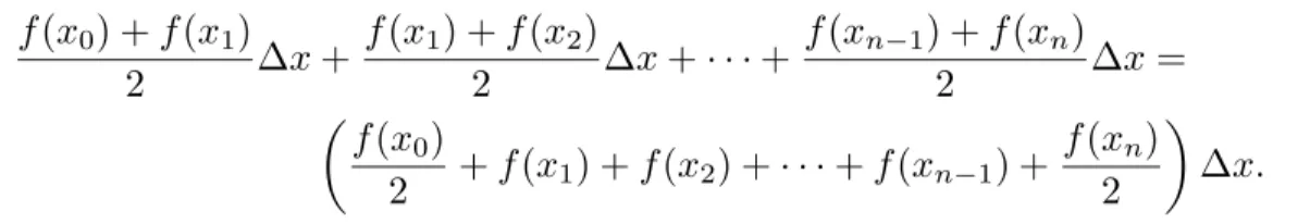
10.5 Numerical Integration 219 by using something other than a straight line? The obvious candidate is a parabola: if we can approximate a short piece of the curve with a parabola with equationy =ax2+bx+c, we can easily compute the area under the parabola.
There are an infinite number of parabolas through any two given points, but only one through three given points. If we find a parabola through three consecutive points (xi, f(xi)), (xi+1, f(xi+1)), (xi+2, f(xi+2)) on the curve, it should be quite close to the
curve over the whole interval [xi, xi+2], as in figure 10.5.3. If we divide the interval [a, b]
into an even number of subintervals, we can then approximate the curve by a sequence of parabolas, each covering two of the subintervals. For this to be practical, we would like a simple formula for the area under one parabola, namely, the parabola through (xi, f(xi)),
(xi+1, f(xi+1)), and (xi+2, f(xi+2)). That is, we should attempt to write down the parabola
y = ax2 +bx+c through these points and then integrate it, and hope that the result is fairly simple. Although the algebra involved is messy, this turns out to be possible. The algebra is well within the capability of a good computer algebra system like Sage, so we will present the result without all of the algebra; you can see how to do it in this Sage worksheet.
To find the parabola, we solve these three equations for a, b, and c: f(xi) =a(xi+1−∆x)2+b(xi+1−∆x) +c
f(xi+1) =a(xi+1)2+b(xi+1) +c
f(xi+2) =a(xi+1+ ∆x)2+b(xi+1+ ∆x) +c
Not surprisingly, the solutions turn out to be quite messy. Nevertheless, Sage can easily compute and simplify the integral to get
Z xi+1+∆x
xi+1−∆x
ax2+bx+c dx= ∆x
3 (f(xi) + 4f(xi+1) +f(xi+2)). Now the sum of the areas under all parabolas is
∆x
3 (f(x0) + 4f(x1) +f(x2) +f(x2) + 4f(x3) +f(x4) +· · ·+f(xn−2) + 4f(xn−1) +f(xn)) = ∆x
3 (f(x0) + 4f(x1) + 2f(x2) + 4f(x3) + 2f(x4) +· · ·+ 2f(xn−2) + 4f(xn−1) +f(xn)). This is just slightly more complicated than the formula for trapezoids; we need to remember the alternating 2 and 4 coefficients; note thatnmust be even for this to make sense. This approximation technique is referred to asSimpson’s Rule.
xi xi+1 xi+2 (xi, f(xi)) (xi+2, f(xi+2)) ...... ... ... ... ... ... ... ... ... ... ... ... ... ... ... ... ...
Figure 10.5.3 A parabola (dashed) approximating a curve (solid).
THEOREM 10.5.3 Suppose f has a fourth derivative f(4) everywhere on the interval [a, b], and |f(4)(x)| ≤M for all x in the interval. With ∆x = (b−a)/n, an error estimate for Simpson’s approximation is
E(∆x) = b−a
180 M(∆x)
4 = (b−a)5 180n4 M.
EXAMPLE 10.5.4 Let us again approximate Z 1
0 e−x2
dx to two decimal places. The fourth derivative of f = e−x2
is (16x2 − 48x2 + 12)e−x2
; on [0,1] this is at most 12 in absolute value. We begin by estimating the number of subintervals we are likely to need. To get two decimal places of accuracy, we will certainly need E(∆x) <0.005, but taking a cue from our earlier example, let’s require E(∆x)<0.001:
1 180(12) 1 n4 <0.001 200 3 < n 4 2.86≈ [4] r 200 3 < n
So we try n = 4, since we need an even number of subintervals. Then the error estimate is 12/180/44 <0.0003 and the approximation is
(f(0) + 4f(1/4) + 2f(1/2) + 4f(3/4) +f(1)) 1
3·4 ≈0.746855.
So the true value of the integral is between 0.746855−0.0003 = 0.746555 and 0.746855 + 0.0003 = 0.7471555, both of which round to 0.75.
10.6 Additional exercises 221
Exercises 10.5.
In the following problems, compute the trapezoid and Simpson approximations using 4 subin-tervals, and compute the error estimate for each. (Finding the maximum values of the second and fourth derivatives can be challenging for some of these; you may use a graphing calculator or computer software to estimate the maximum values.) If you have access to Sage or similar software, approximate each integral to two decimal places. You can use this Sage worksheet to get started. 1. Z 3 1 x dx ⇒ 2. Z 3 0 x2dx⇒ 3. Z 4 2 x3dx⇒ 4. Z 3 1 1 x dx⇒ 5. Z 2 1 1 1 +x2 dx⇒ 6. Z 1 0 x√1 +x dx ⇒ 7. Z 5 1 x 1 +xdx ⇒ 8. Z 1 0 p x3+ 1dx ⇒ 9. Z 1 0 p x4+ 1dx ⇒ 10. Z 4 1 p 1 + 1/x dx⇒
11. Using Simpson’s rule on a parabolaf(x), even with just two subintervals, gives the exact value of the integral, because the parabolas used to approximate f will be f itself. Remarkably, Simpson’s rule also computes the integral of a cubic function f(x) = ax3
+bx2
+cx+d
exactly. Show this is true by showing that
Z x2
x0
f(x)dx= x2−x0
3·2 (f(x0) + 4f((x0+x2)/2) +f(x2)). This does require a bit of messy algebra, so you may prefer to use Sage.
10.6 Additional exerises
These problems require the techniques of this chapter, and are in no particular order. Some problems may be done in more than one way.
1. Z (t+ 4)3dt⇒ 2. Z t(t2−9)3/2dt⇒ 3. Z (et2 + 16)tet2dt⇒ 4. Z sintcos 2t dt ⇒ 5. Z tantsec2t dt ⇒ 6. Z 2t+ 1 t2+t+ 3dt⇒ 7. Z 1 t(t2 −4)dt⇒ 8. Z 1 (25−t2)3/2dt⇒ 9. Z cos 3t √ sin 3tdt⇒ 10. Z tsec2t dt ⇒ 11. Z et √ et+ 1dt⇒ 12. Z cos4t dt ⇒
13. Z 1 t2+ 3tdt⇒ 14. Z 1 t2√1 +t2dt⇒ 15. Z sec2 t (1 + tant)3dt⇒ 16. Z t3p t2+ 1dt ⇒ 17. Z etsint dt ⇒ 18. Z (t3/2+ 47)3√t dt ⇒ 19. Z t3 (2−t2)5/2dt ⇒ 20. Z 1 t(9 + 4t2) dt⇒ 21. Z arctan 2t 1 + 4t2 dt⇒ 22. Z t t2+ 2t −3dt⇒ 23. Z sin3tcos4t dt ⇒ 24. Z 1 t2 −6t+ 9dt⇒ 25. Z 1 t(lnt)2 dt⇒ 26. Z t(lnt)2dt⇒ 27. Z t3etdt⇒ 28. Z t+ 1 t2+t −1dt⇒