Tutorial for the WGCNA package for R: I. Network analysis of liver expression data in female mice

Tutorial for the WGCNA package for R:

I. Network analysis of liver expression data in female mice

2.b Step-by-step network construction and module detection

Peter Langfelder and Steve Horvath

November 25, 2014

Contents

0 Preliminaries: setting up the R session 1

2 Step-by-step construction of the gene network and identification of modules 2

2.b Step-by-step network construction and module detection . . . 2

2.b.1 Choosing the soft-thresholding power: analysis of network topology . . . 2

2.b.2 Co-expression similarity and adjacency . . . 3

2.b.3 Topological Overlap Matrix (TOM) . . . 3

2.b.4 Clustering using TOM . . . 3

2.b.5 Merging of modules whose expression profiles are very similar . . . 5

0

Preliminaries: setting up the R session

Here we assume that a new R session has just been started. We load the WGCNA package, set up basic parameters and load data saved in the first part of the tutorial.

Important note: The code below uses parallel computation where multiple cores are available. This works well when R is run from a terminal or from the Graphical User Interface (GUI) shipped with R itself, but at present it does not workwith RStudio and possibly other third-party R environments. If you use RStudio or other third-party R environments, skip theenableWGCNAThreads()call below.

# Display the current working directory

getwd();

# If necessary, change the path below to the directory where the data files are stored. # "." means current directory. On Windows use a forward slash / instead of the usual \.

workingDir = ".";

setwd(workingDir);

# Load the WGCNA package

library(WGCNA)

# The following setting is important, do not omit.

options(stringsAsFactors = FALSE);

# Allow multi-threading within WGCNA. At present this call is necessary.

# Any error here may be ignored but you may want to update WGCNA if you see one. # Caution: skip this line if you run RStudio or other third-party R environments. # See note above.

enableWGCNAThreads()

# Load the data saved in the first part

#The variable lnames contains the names of loaded variables.

lnames

We have loaded the variablesdatExpr anddatTraitscontaining the expression and trait data, respectively.

2

Step-by-step construction of the gene network and identification of

modules

This step is the bedrock of all network analyses using the WGCNA methodology. We present three different ways of constructing a network and identifying modules:

a. Using a convenient 1-step network construction and module detection function, suitable for users wishing to arrive at the result with minimum effort;

b. Step-by-step network construction and module detection for users who would like to experiment with cus-tomized/alternate methods;

c. An automatic block-wise network construction and module detection method for users who wish to analyze data sets too large to be analyzed all in one.

In this tutorial section, we illustrate the step-by-step network construction and module detection.

2.b

Step-by-step network construction and module detection

2.b.1 Choosing the soft-thresholding power: analysis of network topology

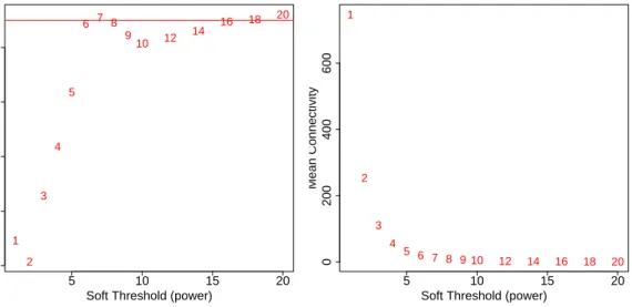
Constructing a weighted gene network entails the choice of the soft thresholding power β to which co-expression similarity is raised to calculate adjacency [1]. The authors of [1] have proposed to choose the soft thresholding power based on the criterion of approximate scale-free topology. We refer the reader to that work for more details; here we illustrate the use of the functionpickSoftThresholdthat performs the analysis of network topology and aids the user in choosing a proper soft-thresholding power. The user chooses a set of candidate powers (the function provides suitable default values), and the function returns a set of network indices that should be inspected, for example as follows:

# Choose a set of soft-thresholding powers

powers = c(c(1:10), seq(from = 12, to=20, by=2))

# Call the network topology analysis function

sft = pickSoftThreshold(datExpr, powerVector = powers, verbose = 5)

# Plot the results:

sizeGrWindow(9, 5) par(mfrow = c(1,2)); cex1 = 0.9;

# Scale-free topology fit index as a function of the soft-thresholding power

plot(sft$fitIndices[,1], -sign(sft$fitIndices[,3])*sft$fitIndices[,2],

xlab="Soft Threshold (power)",ylab="Scale Free Topology Model Fit,signed R^2",type="n",

main = paste("Scale independence"));

text(sft$fitIndices[,1], -sign(sft$fitIndices[,3])*sft$fitIndices[,2],

labels=powers,cex=cex1,col="red");

# this line corresponds to using an R^2 cut-off of h

abline(h=0.90,col="red")

# Mean connectivity as a function of the soft-thresholding power

plot(sft$fitIndices[,1], sft$fitIndices[,5],

xlab="Soft Threshold (power)",ylab="Mean Connectivity", type="n",

main = paste("Mean connectivity"))

text(sft$fitIndices[,1], sft$fitIndices[,5], labels=powers, cex=cex1,col="red")

The result is shown in Fig. 1. We choose the power 6, which is the lowest power for which the scale-free topology fit index reaches 0.90.

5 10 15 20 0.0 0.2 0.4 0.6 0.8 Scale independence

Soft Threshold (power)

Scale Free Topology Model Fit,signed R^2 1 2 3 4 5 6 7 8 9 10 12 14 16 18 20 5 10 15 20 0 200 400 600 Mean connectivity

Soft Threshold (power)

Mean Connectivity 1 2 3 4 5 6 7 8 9 10 12 14 16 18 20

Figure 1: Analysis of network topology for various soft-thresholding powers. The left panel shows the scale-free fit index (y-axis) as a function of the soft-thresholding power (x-axis). The right panel displays the mean connectivity (degree,y-axis) as a function of the soft-thresholding power (x-axis).

2.b.2 Co-expression similarity and adjacency

We now calculate the adjacencies, using the soft thresholding power 6: softPower = 6;

adjacency = adjacency(datExpr, power = softPower);

2.b.3 Topological Overlap Matrix (TOM)

To minimize effects of noise and spurious associations, we transform the adjacency into Topological Overlap Matrix, and calculate the corresponding dissimilarity:

# Turn adjacency into topological overlap

TOM = TOMsimilarity(adjacency); dissTOM = 1-TOM

2.b.4 Clustering using TOM

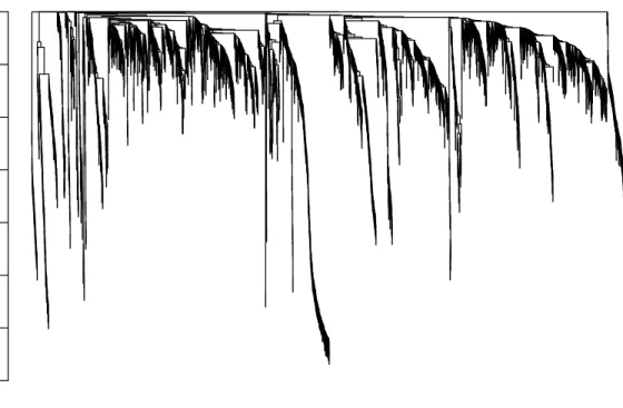
We now use hierarchical clustering to produce a hierarchical clustering tree (dendrogram) of genes. Note that we use the function hclustthat provides a much faster hierarchical clustering routine than the standardhclustfunction.

# Call the hierarchical clustering function

geneTree = hclust(as.dist(dissTOM), method = "average");

# Plot the resulting clustering tree (dendrogram)

sizeGrWindow(12,9)

plot(geneTree, xlab="", sub="", main = "Gene clustering on TOM-based dissimilarity",

labels = FALSE, hang = 0.04);

The clustering dendrogram plotted by the last command is shown in Figure 2. In the clustering tree (dendrogram), each leaf, that is a short vertical line, corresponds to a gene. Branches of the dendrogram group together densely interconnected, highly co-expressed genes. Module identification amounts to the identification of individual branches (”cutting the branches off the dendrogram”). There are several methods for branch cutting; our standard method is the Dynamic Tree Cut from the package dynamicTreeCut. The next snippet of code illustrates its use.

0.3 0.4 0.5 0.6 0.7 0.8 0.9 1.0

Gene clustering on TOM−based dissimilarity

Height

Figure 2: Clustering dendrogram of genes, with dissimilarity based on topological overlap.

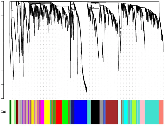
# We like large modules, so we set the minimum module size relatively high:

minModuleSize = 30;

# Module identification using dynamic tree cut:

dynamicMods = cutreeDynamic(dendro = geneTree, distM = dissTOM, deepSplit = 2, pamRespectsDendro = FALSE,

minClusterSize = minModuleSize); table(dynamicMods)

The function returned 22 modules labeled 1–22 largest to smallest. Label 0 is reserved for unassigned genes. The above command lists the sizes of the modules. We now plot the module assignment under the gene dendrogram:

# Convert numeric lables into colors

dynamicColors = labels2colors(dynamicMods) table(dynamicColors)

# Plot the dendrogram and colors underneath

sizeGrWindow(8,6)

plotDendroAndColors(geneTree, dynamicColors, "Dynamic Tree Cut",

dendroLabels = FALSE, hang = 0.03, addGuide = TRUE, guideHang = 0.05,

main = "Gene dendrogram and module colors")

0.3 0.4 0.5 0.6 0.7 0.8 0.9 1.0

Gene dendrogram and module colors

hclust (*, "average") as.dist(dissTom)

Height

Dynamic Tree Cut

Figure 3: Clustering dendrogram of genes, with dissimilarity based on topological overlap, together with assigned module colors.

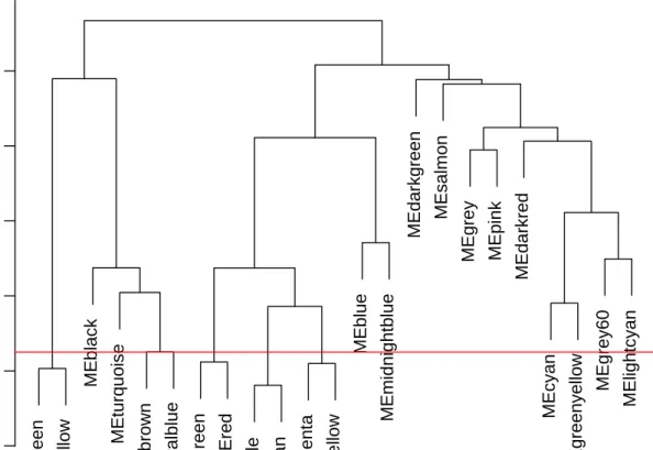
2.b.5 Merging of modules whose expression profiles are very similar

The Dynamic Tree Cut may identify modules whose expression profiles are very similar. It may be prudent to merge such modules since their genes are highly co-expressed. To quantify co-expression similarity of entire modules, we calculate their eigengenes and cluster them on their correlation:

# Calculate eigengenes

MEList = moduleEigengenes(datExpr, colors = dynamicColors) MEs = MEList$eigengenes

# Calculate dissimilarity of module eigengenes

MEDiss = 1-cor(MEs);

# Cluster module eigengenes

METree = hclust(as.dist(MEDiss), method = "average");

# Plot the result

sizeGrWindow(7, 6)

plot(METree, main = "Clustering of module eigengenes",

xlab = "", sub = "")

MEDissThres = 0.25

# Plot the cut line into the dendrogram

abline(h=MEDissThres, col = "red")

# Call an automatic merging function

merge = mergeCloseModules(datExpr, dynamicColors, cutHeight = MEDissThres, verbose = 3)

# The merged module colors

mergedColors = merge$colors;

# Eigengenes of the new merged modules:

mergedMEs = merge$newMEs;

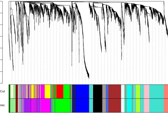
To see what the merging did to our module colors, we plot the gene dendrogram again, with the original and merged module colors underneath (Figure 5).

sizeGrWindow(12, 9)

#pdf(file = "Plots/geneDendro-3.pdf", wi = 9, he = 6)

plotDendroAndColors(geneTree, cbind(dynamicColors, mergedColors), c("Dynamic Tree Cut", "Merged dynamic"), dendroLabels = FALSE, hang = 0.03, addGuide = TRUE, guideHang = 0.05)

#dev.off()

In the subsequent analysis, we will use the merged module colors inmergedColors. We save the relevant variables for use in subsequent parts of the tutorial:

# Rename to moduleColors

moduleColors = mergedColors

# Construct numerical labels corresponding to the colors

colorOrder = c("grey", standardColors(50));

moduleLabels = match(moduleColors, colorOrder)-1; MEs = mergedMEs;

# Save module colors and labels for use in subsequent parts

save(MEs, moduleLabels, moduleColors, geneTree, file = "FemaleLiver-02-networkConstruction-stepByStep.RData")

References

[1] B. Zhang and S. Horvath. A general framework for weighted gene co-expression network analysis. Statistical Applications in Genetics and Molecular Biology, 4(1):Article 17, 2005.

MElightgreen

_{MElightyellow}

MEblack

MEturquoise

MEbrown

MEroyalblue

MEgreen

MEred

MEpurple

MEtan

MEmagenta

MEyellow

MEblue

MEmidnightblue

MEdarkgreen

MEsalmon

MEgrey

MEpink

MEdarkred

MEcyan

MEgreenyellow

MEgrey60

MElightcyan

0.0

0.2

0.4

0.6

0.8

1.0

Consensus clustering of consensus module eigengenes

Height

Figure 4: Clustering dendrogram of genes, with dissimilarity based on topological overlap, together with assigned merged module colors and the original module colors.

0.3 0.4 0.5 0.6 0.7 0.8 0.9 1.0

Cluster Dendrogram

Dynamic Tree Cut

Merged dynamic

Figure 5: Clustering dendrogram of genes, with dissimilarity based on topological overlap, together with assigned merged module colors and the original module colors.