Sharif University of Technology
Scientia IranicaTransactions A: Civil Engineering www.scientiairanica.com
Research Note
Numerical simulation of ow over spillway based on the
CFD method
E. Fadaei-Kermani
and G.A. Barani
Department of Civil Engineering, Shahid Bahonar University, Kerman, P. O. Box 76169133, Iran. Received 31 August 2012; received in revised form 25 April 2013; accepted 13 August 2013
KEYWORDS Spillway; Numerical modeling; CFD method; RNG model; Flow characteristics.
Abstract. In this study, numerical simulation of ow over a chute spillway is presented using the Computational Fluid Dynamics (CFD) method. The ow characteristics such as velocity, pressure and depth through the spillway have been calculated for four dierent ow rates. Since the actual ow is turbulent, the RNG turbulence model has been used for simulation. The numerical computed results of piezometric pressure and ow velocity along the spillway were compared with the results from the hydraulic model tests. The maximum dierence between calculated and experimental results in average velocity values was 5.47% and in piezometric pressure values was 7.97%. The numerical results agreed well with experiments.
c
2014 Sharif University of Technology. All rights reserved.
1. Introduction
A spillway is one of the most important hydraulic structures designed to prevent overtopping of dams and provide sucient safety and stability during oods. Improper design of spillways may cause failure in dams; consequently, the spillway must be carefully designed and hydraulically adequate to verify the ow characteristics [1].
Analysis of ow over a spillway can be an im-portant engineering problem. Therefore, recent devel-opments in computer science and numerical techniques have advanced the use of Computational Fluid Dynam-ics (CFD) as a powerful tool for this purpose.
Computational Fluid Dynamics (CFD) is a type of numerical method used to solve problems involving uid ow. Since CFD can provide a faster and more economical solution than physical models, engineers are interested in verifying the capability of CFD software [2]. Some recent works show the capability of the CFD method in the numerical modeling of
*. Corresponding author.
E-mail address: [email protected] (E. Fadaei)
ow over several spillways. Savage and Johnson [3] simulated ow over a standard ogee-crest spillway using a commercial CFD code (ow-3D). They found good agreement between the physical and numerical models for both pressures and discharges. Ho et al. [4] described the two- and three-dimensional CFD modeling of spillway behavior under rising ood levels. The results were validated using published data, and acceptable results were obtained. Kim and Park [5] investigated ow characteristics on the ogee spillway using ow-3D software. They found that the scale eects on the model are in an acceptable error range if the length scale ratio is less than 100 or 200. Dargahi [6] did a three- dimensional simulation of ow over a spillway by means of CFD software (Fluent). He predicted the water surface proles and the discharge coecients for a laboratory spillway within an accu-racy range of 1.5-2.9%, depending on the spillway's operating head. Zhenwei et al. [7] simulated ow over the whole spillway based on the VOF model using Fluent software. They found reasonable agreement between numerical and experimental results for the surface elevation, pressure and ow velocity along the spillway.
Table 1. Some features of the Shahid Abbaspour dam. Type Height (m) Length (m) Reservoir capacity (m3) Type of spillway Spillway capacity (m3/s) Maximum water level (m) Double-curvature concrete
200 380 3000 million Gated ski-chute 16500 530
In this study, to investigate ow characteristics over the whole spillway, the CFD software, ow-3D, has been used. Moreover, the ability of this software has been examined with regard to a spillway conguration by comparing the results with experimental results. 2. Experimental model
The Shahid Abbaspour dam is a large arch dam on the Karun River located 50 kilometers northeast of Masjed Soleiman, in Khuzesten province, Iran. Some features of this dam are presented in Table 1.
The chute spillway consists of three bays with a width of 18.5 m, which are controlled by radial gates, 2015 m in dimension [8]. The hydraulic model of this spillway was built in the hydraulic laboratory of the Iran Water Research Institute (WRI) in 1984, with a scale of 1:62.5. The spillway hydraulic model consists of part of the dam, spillway conguration, and radial gates; 250 meters from the lake upstream and 800 meters from the river downstream [9]. Based on several measurements, values of water depth, velocity and piezometric pressure were calculated along the spillway for dierent water levels.
3. Numerical methodology
Flow-3D is a powerful CFD software, capable of solving a wide range of uid ow problems. It uses the nite volume method to solve RANS (Reynolds Average Navier-Stokes) equations. This software utilizes a true Volume Of Fluid method (VOF method) for comput-ing free surface motion [10], and complex geometric regions are modeled using the area/volume obstacle representation (FAVOR) method [11]. In the true VOF method, a special advection technique is used that gives a sharp denition of the free surface and does not compute the dynamics in the void or air regions. The portion of volume or area occupied by the obstacle in each cell is dened at the beginning of the analysis, and the uid fraction in each cell is also calculated. The continuity and momentum equations of the uid fraction are formulated using the FAVOR function, and the nite volume method or a nite dierence approximation is used for the discretization and solving of each equation [4].
The general governing mass continuity equation,
including the VOF and FAVOR variables, can be written as:
VF@p@t +@x@ (uAx) + R@y@ (vAy) +@z@ (wAz)
+ uAxx = RDIF+ RSOR; (1)
where VF is the fractional volume open to ow, is
the uid density, RDIF is a turbulent diusion term,
and RSOR is a mass source. The velocity components
(u; v; w) can be in the coordinate directions (x; y; z) or (r; ; z). Ax; Ay and Az are the fractional areas open
to ow in x ; y and z directions, respectively. The rst term on the right side of Eq. (1) is a turbulent diusion term:
RDIF=@x@ (Ax@p@x) + R@y@ (AyR@p@y)
+@z@ (Az@z@p) + xAx; (2)
where the coecient = C= in which is the
coecient of momentum diusion, and Cpis a constant
whose reciprocal is usually referred to as the turbulent Schmidt number. Finally, the last term, RSOR, on the
right side of Eq. (1), is a density source term that can be used, for example, to model mass injection through porous obstacle surfaces [12].
In compressible ow problems, solution of the full density transport equation is required, as stated in Eq. (1). For incompressible ow problems, is a constant and Eq. (1) reduces to the incompressibility condition:
@ @x(uAx)+ R @ @y(Ay) + @ @z(wAz)+ uAx x = RSOR (3): The equations of motion for the uid velocity compo-nents (u; v; w) in the three coordinate directions (the Navier-Stokes equations) can be written as:
@u @t + 1 VF uAx@u@x + vAyR@u@y + wAz@u@z AxVyv2 F = 1 @p @x + Gx+ fx bx RSOR VF u;
@v @t + 1 VF uAx@v@x+ vAyR@v@y+ wAz@v@z + Ayuv xVF = 1 R @p @y + Gy+ fy by RSOR VF v; @w @t + 1 VF uAx@w@x + vAyR@w@y + wAz@w@z = 1@p@z + Gz+ fz bz RVSOR F w; (4)
where (Gx; Gy; Gz) are body accelerations, (fx; fy; fz)
are viscous accelerations, (bx; by; bz) are ow losses in
porous medium, and the nal terms account for the injection of mass at a source represented by geometry components. The term Uw = (uw; vw; ww) is the
velocity of the source component, and the term Us=
(us; vs; ws) is the velocity of the uid at the surface of
the source relative to the source itself [12].
As mentioned before, ow-3D numerically solves the governing equations using nite dierence or nite volume approximations. The ow region is subdivided into rectangular cells. With each cell, there are associated local average values of dependent variables. The basic numerical method used in this software has a formal accuracy, using rst order nite dier-ence approximations with respect to time and space increments. Special precautions have been taken to maintain this degree of accuracy, even when the nite dierence mesh is not uniform. Moreover, second order accurate options are also available. In any case, boundary conditions are at least rst order accurate in all circumstances [12].
For example, a generic form for the nite dier-ence approximation of the momentum equation (Eq. (4)) can be written as:
un+1 i;j;k=uni;j;k+ tn+1[ Pn=1 i+1;j;k Pi;j;kn=1 (x)n i+1 2;j;k
+Gx-FUX -FUY -FUZ +VISX-BX -WSX];
vn+1 i;j;k=vi;j;kn + tn+1[ Pn=1 i;j+1;k Pi;j;kn=1 (y)n i+1 2;j;k :Ri+1 2
+ Gy -FVX -FVY -FVZ+VISY -BY -WSY];
wn+1 i;j;k=wni;j;k+ tn+1[ Pn=1 i;j;k+1 Pi;j;kn=1 (x)n i+1 2;j;k +Gz-FWX-FWY-FWZ +VISZ-BZ-WSZ]; (5) where Ri+1=2 is related to coordinate systems and
equals 1 in Cartesian coordinates. The advective,
vis-cous and acceleration terms have an obvious meaning. For example, FUX means the advective ux of u in the x direction; VISX is the x component viscous acceleration; BX is the ow losses for a bae normal to the x direction; WSX is the viscous wall acceleration in the x-direction, and GX includes gravitational, rotational and general non-inertial accelerations. 4. Numerical model implementation
Flow over the Shahid Abbaspour dam spillway was modeled using the ow-3D software. The geometry of the spillway was created by Auto-Cad software and exported as a stereolithographic (stl) format. Then, the stl le was directly imported into the ow-3D.
The computational domain includes 150 meters before the spillway crest, the whole spillway structure and 300 meters after the ip-bucket. Moreover, about 50 meters above the spillway crest have been considered in the computational domain in a vertical direction. The renormalization group (RNG) turbulence model has been used for simulation. The decision was made based on comments in the ow-3D user's manual [12], that the RNG turbulence model is the most accurate model available in ow-3D software.
Setting the appropriate boundary conditions has a signicant eect on whether the numerical results are reecting the actual situation. As the ow domain in this software is dened as a hexahedral in Cartesian coordinates, there are six dierent boundaries to be xed. In this case, ow data from free surface ow are desired. Therefore, in a vertical direction, the top boundary was set as atmospheric pressure, and the bottom boundary was specied as the wall. Since the purpose of these simulations is to model ow rate over a spillway with dierent water head levels for comparison with physical model data, the upstream boundary was set as the specied pressure based on total uid height over the spillway crest, while the downstream boundary was set as outow. It is to be mentioned that there are also several other boundary options available in this software that could be applied to the downstream side. The boundary condition in the y-direction or the direction perpendicular to the ow is specied as the wall on both sides. Figure 1 shows the boundary conditions set at each direction.
Implementing accurate initial conditions as closely as possible to the actual ow eld has a very important eect on simulation times [2]. Rectangular regions were specied at the upstream and downstream of the spillway for the initial condition, and the pressure considered as hydrostatic distribution in the vertical direction. Rectangular uid regions were specied on the downstream and upstream sides of the spillway at the same level as the specied uid height at bound-aries. Figure 2 shows the situation of the spillway at
Figure 1. The boundary conditions set at each direction.
Figure 2. The situation of the spillway at the beginning of the analysis.
the beginning of the analysis. In this case, the specied uid height was considered 181.2 m, to provide a ow rate of 1370 m3/s.
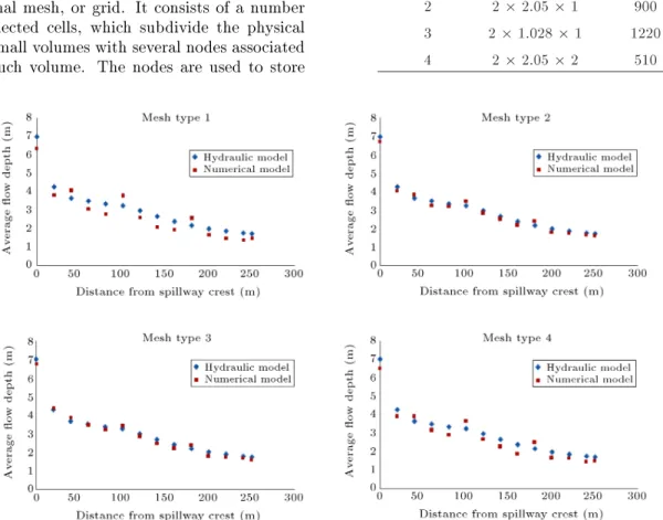
Typically, every numerical model starts with a computational mesh, or grid. It consists of a number of interconnected cells, which subdivide the physical space into small volumes with several nodes associated with each such volume. The nodes are used to store
values of the unknown parameters, such as pressure and velocity. Determining the appropriate grid size is also an important part of any numerical simulation. Grid size can aect not only the accuracy of results, but also simulation time. Therefore, it is important to minimize the number of grids while including enough resolution to suciently acquire signicant features of geometry and the ow details. In this study, four dierent mesh types were considered. The size of grids and the corresponding calculation time for each mesh type are presented in Table 2. The accuracy of each mesh type compared with experimental results is shown in Figure 3. The results have been pre-sented based on average ow depth in the discharge of 1370 m3/s.
According to the accuracy of computed results and corresponding simulation time for each mesh type, mesh type two has been selected for the rest of the simulation, and numerical results have been presented based on this mesh size.
Table 2. The mesh type and the corresponding calculation time. Mesh type Mesh size (x y z) (m) Calculation time (min) 1 42.05 2 290 2 2 2.05 1 900 3 2 1.028 1 1220 4 2 2.05 2 510
5. Results
By three-dimensional numerical simulation, ow char-acteristics such as ow depth, velocity and pressure were obtained under the condition of four dierent ow rates. Results have been compared with the experimental results of the hydraulic model.
The piezometric pressure values along the spillway were calculated for four dierent ow rates. Figures 4 to 7 show the pressure proles along the spillway. It can be seen that there is reasonably good agreement be-tween the results of the numerical model and those from experiments. For all ow rates, the minimum pressure
Figure 4. Comparison of computed and measured piezometric pressure for Q = 1370 m3/s.
Figure 5. Comparison of computed and measured piezometric pressure for Q = 2000 m3/s.
Figure 6. Comparison of computed and measured piezometric pressure for Q = 2500 m3/s.
on the chute occurs at a distance of 140 meters from the spillway crest. The pressure drop at this section of the chute may cause a cavitation phenomenon that can be harmful for the structure. The dierence percentage between computed and measured piezometric pressure values is presented in Table 3. It can be seen that the maximum dierence is 7.97%, and the values match well.
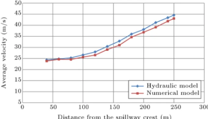
For all ow rates, the average velocity proles calculated by the numerical model and measured by the hydraulic model are shown in Figures 8 to 11. According to the results, we discover that as the
Figure 7. Comparison of computed and measured piezometric pressure for Q = 3000 m3/s.
Figure 8. Comparison of computed and measured average ow velocity for Q = 1370 m3/s.
Figure 9. Comparison of computed and measured average ow velocity for Q = 2000 m3/s.
Table 3. Dierence between computed and measured piezometric pressure (%).
Distance from Dierence (%)
spillway crest (m) Q = 1370 m3/s Q = 2000 m3/s Q = 2500 m3/s Q = 3000 m3/s 40 4.19 2.8 2.72 3.18 60 6.68 4.46 3.18 4.2 80 7.39 7.76 5.26 3.3 100 4.88 7.82 7.94 7.47 120 4.09 7.56 1.66 4.5 140 7.89 6.83 5.27 4.15 160 4.67 6.75 4.42 7.94 180 7.96 7.07 7.74 7.88 200 7.29 7.79 4.85 4.7 220 7.93 5.63 6.74 7.92 240 7.97 7.94 6.29 6.86 250 7.89 5.64 7.82 7.46
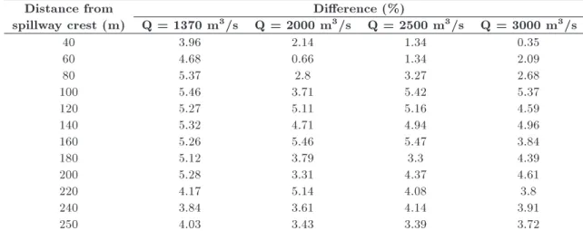
Table 4. Dierence between computed and measured ow velocity (%).
Distance from Dierence (%)
spillway crest (m) Q = 1370 m3/s Q = 2000 m3/s Q = 2500 m3/s Q = 3000 m3/s 40 3.96 2.14 1.34 0.35 60 4.68 0.66 1.34 2.09 80 5.37 2.8 3.27 2.68 100 5.46 3.71 5.42 5.37 120 5.27 5.11 5.16 4.59 140 5.32 4.71 4.94 4.96 160 5.26 5.46 5.47 3.84 180 5.12 3.79 3.3 4.39 200 5.28 3.31 4.37 4.61 220 4.17 5.14 4.08 3.8 240 3.84 3.61 4.14 3.91 250 4.03 3.43 3.39 3.72
Figure 10. Comparison of computed and measured average ow velocity for Q = 2500 m3/s.
ow rate increases, the ow velocity increases also. Moreover, because of the high ow velocity at the ending areas of the chute, these areas might be at risk of serious to major cavitation damage [13]. The dier-ence percentage between calculated and experimental results is presented in Table 4. It can be seen that the maximum dierence between results is 5.47%, which is
Figure 11. Comparison of computed and measured average ow velocity for Q = 3000 m3/s.
less than 6% [7], and the calculated values match well with experimental results.
6. Conclusion
As physical measurements are expensive and time con-suming, numerical modeling can be a convenient and
eective tool for analyzing ow over spillways. Using numerical modeling can provide detailed information of the complete ow eld and ensure the correctness of the design.
In this study, ow over a chute spillway was simulated using CFD software, ow-3D. It was seen that the numerical results agreed well with experi-ments. The maximum dierence between calculated and experimental results in average velocity values was 5.47% and, in piezometric pressure values, was 7.97%. Evaluation of the capability of this software for numerical simulation of ow over a spillway proved to be successful.
References
1. Khatsuria, R.M. \Hydraulics of spillways and energy dissipators", 1st Ed., pp. 2-15, Marcel Dekker, New York, USA (2005).
2. Chanel, P.G. \An evaluation of computational uid dynamics for spillways", Thesis (MSC), University of Manitoba, Canada, pp. 11-23 (2008).
3. Savage, B.M. and Johnson, M.C. \Flow over ogee spillway: Physical and numerical model case study", J. of Hydraul. Eng., ASCE, 127(8), pp. 640{649 (2001).
4. Ho, H., Boyes, K., Donohoo, S. and Cooper, B. \Numerical ow analysis for spillways", Proc., 43rd ANCOLD Conf., Hobart, Tasmania, pp. 24-29 (2003).
5. Kim, D.G., and Park, J.H. \Analysis of ow structure over ogee spillway in consideration of scale and rough-ness eect by using CFD model", J. of Civil Eng., KSCE, 9(2), pp. 161-169 (2005).
6. Dargahi, B. \Experimental study and 3D numerical simulations for a free-overow spillway", J. of Hydraul. Eng., ASCE, 132(9), pp. 899-907 (2006).
7. Zhenwei, M., Zhiyan, Z. and Tao, Z. \Numerical simulation of 3-D ow eld of spillway based on VOF method ", Procedia Engineering, 28, pp. 808-812 (2012).
8. Mahab Ghodss Consulting Engineers, Karun Model Spillway, Hydraulic Department, Tehran (1984).
9. Water Research Institute, Iran Ministry of Energy, Hydraulic Model of the Spillway of Shahid Abbaspour Dam, Dept. of Hydro-Environment, Tehran, Iran (1984).
10. Hirt, C.W. and Nichols, B.D. \Volume of Fluid (VOF) method for the dynamics of free boundaries", J. Comp. Phys., 39(1), pp. 201-225 (1981).
11. Hirt, C.W. and Sicilian, J.M. \A porosity technique for the denition of obstacles in rectangular cell meshes"., Proc. 4th Int. Conf. Ship Hydro, National Academy of Science, Washington, DC, September, pp. 1-19 (1985).
12. Flow Science, Inc. \Flow-3D user's manuals, version 9.2", pp. 110-114, Santa Fe, NM (2007).
13. Fadaei Kermani, E., Barani, G.A., and Ghaeini-Hessaroeyeh., M. \Investigation of cavitation damage levels on spillways", World Applied Sciences Journal, 21(1), pp. 73-78 (2013).
Biographies
Ehsan Fadaei Kermani received his BS degree in Civil Engineering from Shahid Bahonar University of Kerman in 2010 and his MS degree in Hydraulic Structures in 2012. His research interests include computational uid dynamics, data mining and arti-cial intelligence approaches. He has published and presented papers in various journals and at national and international conferences.
Gholam Abbas Barani received his BS degree in Civil Engineering from Tehran University in 1973, and received his MS degree in 1977 from the University of California, Davis, where he continued his research work towards a PhD degree. His research interests include sediment scour in hydraulic structures, water resource engineering, optimization of reservoir operation, and hydrology. He has published more than 300 papers in various journals and presented many others at national and international conferences.