A Global Constraint for Bin-Packing with Precedences:
Application to the Assembly Line Balancing Problem.
Pierre Schaus
and
Yves Deville
Department of Computing Science and Engineering,University of Louvain, Place Sainte Barbe 2, B-1348 Louvain-la-Neuve, Belgium
{pierre.schaus,yves.deville}@uclouvain.be
Abstract
Assembly line balancing problems (ALBP) are of capital im-portance for the industry since the first assembly line for the Ford T by Henry Ford. Their objective is to optimize the design of production lines while satisfying the various con-straints. Precedence constraints among the tasks are always present in ALBP. The objective is then to place the tasks among various workstations such that the production rate is maximized. This problem can be modeled as a bin pack-ing problem with precedence constraints (BPPC) where the bins are the workstations and the items are the tasks. Paul Shaw introduced a global constraint for bin-packing (with-out precedence). Unfortunately this constraint does not cap-ture the precedence constraints of BPPC. In this paper, we first introduce redundant constraints for BPPC combining the precedences and the bin-packing, allowing to solve instances which are otherwise intractable in constraint programming. We also design a global constraint for BPPC, introducing even more pruning in the search tree. We finally used our CP model for BPPC to solve ALBP. We propose two search heuristics, and show the efficiency of our approach on stan-dard ALBP benchmarks. Compared to stanstan-dard non CP ap-proaches, our method is more flexible as it can handle new constraints that might appear in real applications.
Introduction
In a variant of the bin packing problem, items of different volume must be packed into a finite number of bins with a fixed capacity in a way that balances the load of the differ-ent bins (e.g. minimizes the maximum load of the bins). We are interested in bin packing problems with precedence con-straints between items (BPPC). Here the bins are ordered. A precedence constraint between itemsa1anda2is satisfied if itema1is placed in a binB1, and itema2in a binB2, with B1≤B2.
BPPC occurs frequently in the design of assembly lines in the industry1. We are given a set of tasks of various
lengths, subject to precedence constraints, and a time con-stant called cycle time. The problem is to distribute the tasks over workstations along a production (assembly) line, so that no workstation takes longer than the cycle time to complete Copyright c2008, Association for the Advancement of Artificial Intelligence (www.aaai.org). All rights reserved.
1
See for example the two commercial softwares Proplannerr
www.proplanner.comand OptiLinerwww.optimaldesign.com
all the tasks assigned to it (station time), and the precedence constraints are satisfied. The decision problem of optimally partitioning (balancing) the tasks among the stations with respect to some objective is called the assembly line bal-ancing problem (ALBP) (Boysen, Fliedner, & Scholl 2007; Scholl & Becker 2006).
In particular, when the number of stations is fixed, the problem is to distribute the tasks to stations such that the station time is balanced, that is to minimize the cycle time. This type of problems is usually called Simple ALBP-2 (SALBP-2) (Boysen, Fliedner, & Scholl 2007). It is clear that SALBP-2 and BPPC are equivalent.
BPPC and SALBP-2 can be solved by exact or heuris-tic methods. In this paper, we are interested inexact meth-ods. Existing exact methods are usually dedicated branch and bound algorithms such as Salome 2 (Klein & Scholl 1996). These algorithms are very efficient and have been improved since about 50 years. Unfortunately these algo-rithms are not flexible to new constraints that might ap-pear in real applications such as minimal distance between two tasks or restriction on the cumulated value of a partic-ular task attribute (see the problem classifier available on www.assembly-line-balancing.de for more details). When such constraints are added, we obtain so-called Generalized Assembly Line Balancing Problems (GALBP) (Becker & Scholl 2006). The existing exact methods are not flexible enough to handle GALBP efficiently. The Constraint Pro-gramming (CP) paradigm is a good candidate to tackle such problems since constraints can be added very easily to the model.
The Constraint Programming (CP) framework has already been used for the bin packing problem (e.g. (Shaw 2004)). The Balanced Academic Curriculum Problem (BACP) is equivalent to BPPC. The objective is to schedule courses into a given number of periods such that the prerequisites relations between the courses are satisfied and such that the workloads among the periods are well balanced. Basic CP models have been proposed in (Castro & Manzano 2001; Hnich, Kiziltan, & Walsh 2002).
In this paper, we propose a CP model for BPPC and SALBP-2, allowing a flexible expression of new constraints, such as in GALBP. More specifically, our contributions are : • An efficient and simple CP model for the bin packing with
• A new global constraint for BPPC. This constraint is based on set variables, and exploit the transitive closure of the precedence graph. AnO(n2)filtering algorithm is presented, wherenis the number of items (tasks). This constraint allows to solve instances which are otherwise intractable in CP.
• An experimental validation on standard SALBP-2 bench-marks, showing the feasibility, the efficiency, and the flex-ibility of this approach.
The paper is structured as follows. A background on con-straint programming is first given, followed by a CP model for BPPC. A new global constraint and its associated filter-ing algorithm is then described. Before concludfilter-ing this pa-per, an experimental section analyzes the performance of our approach on standard SABLP benchmarks.
CP Background
Constraint Programming is a powerful paradigm for solving Combinatorial Search Problems (CSP). A CSP is composed of a set of variables; each variable having a finite domain of possible values, and a set of constraints on the variables. The objective is to find an assignment of the variables that satisfies all the constraints. An objective function may also be added. CP interleaves a search process (backtracking or branch-and-bound) with inference (also called propagation or filtering), aiming at reducing the search space by remov-ing values that cannot belong to any solution.
Given a finite domain integer variable X with domain Dom(X), we denote byXminandXmaxthe minimum and maximum value of its domain. Set variables in CP (Gervet 1993) allow to represent a set rather than a single value. The domain of a set variableSis represented by two setsSand S withS ⊆ S. The lower boundS represents the values that must be in the set, andSrepresents the values that may figure in the set;i.e. S ⊆ S ⊆ S.
Redundant constraints (also called implied or surrogate constraints) are constraints which are implied by the con-straints defining the problem. They do not change the set of solutions, and hence are logically redundant. Adding redun-dant constraints to the model may however further reduce the search space by allowing more pruning. Redundant con-straints have been successfully applied to various problems such as car sequencing.
A global constraint can be seen as a constraint on a set of variables, modeling a well-defined part of the problem, and with a dedicated filtering algorithm (van Hoeve & Katriel 2006).
CP Models for the Bin Packing with
Precedence Constraints
The bin packing with precedence constraint (BPPC) implies the following parameters and variables :
• npositive values[s1, ..., sn]representing the size of each
item.
• a number of available binsm.
• mvariables[L1, ..., Lm]representing the load of each bin
(Dom(Li) ={0, . . . ,Pisi})
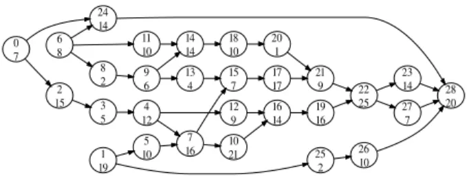
Figure 1: Precedence graph of the Buxey instance from Scholl benchmark data set (Scholl 93).
• nvariables[B1, ..., Bn]representing for each item the bin
where it is placed (Dom(Bi) ={1, . . . , m})
• a precedence (directed and acyclic) graphG({1, .., n}, E) The constraints should model the precedence, and the load of the bins. The objective is to minimize the maximum of the loads,i.e.minimize max{Li}.
The precedence constraints are easily modeled as a set of constraints
Bi≤Bj (with (i, j)∈E) (1)
The simplest way to model the load of each bin is to add binary variablesXij ∈ {0,1}telling whether itemjis
placed into bini. These variables are linked to the variables of the problems through reified constraints:
Xij = 1↔Bj=i. (2)
The loads of each bin is then expressed as a scalar product: Li=
X
j
Xij·sj. (3)
We improve this model with the following redundant con-straint (Shaw 2004): X i Li= X j sj. (4)
The global constraint for bin packing, described in (Shaw 2004) and calledIloPackin Ilog Solver (ILOG-S.A. ), can also be added.
The speedup obtained with the redundant constraints (4) andIloPackis illustrated on a small instance of SALBP-2 from the Scholl benchmark data set (Scholl 93). The prob-lem is to place the items (tasks) into 12 bins (workstations) while satisfying the precedence constraints, given in Figure 1, and minimizing the maximum height of the bins.
Table 1 shows (columns A,B and C) that adding the sim-ple redundant constraint (4) reduces significantly the number of backtracks and time, and that the bin packing constraint from (Shaw 2004) reduces it even more.
New Redundant Constraints for the BPPC
We introduce new redundant constraints improving the fil-tering for BBPC by linking the precedences with the bin packing problem thanks to set variables.We denote byPi the set variable representing the
A B C D #bks time #bks time #bks time #bks time 6894 10.62 4850 7.34 2694 4.3 445 1.07 Table 1: Comparison in terms of backtracks and time (seconds) of the bin packing models on the Buxey instance with 12 worksta-tions. Column A is obtained with the basic model, column B by adding the redundant constraint (4), column C by also adding the IloPackconstraint described in (Shaw 2004) and column D by adding also the redundant constraints (5) and (7).
an itemiif and only if itemjis placed in a bin preceding or equal to the bin of itemi:
j∈ Pi↔Bj ≤Bi. (5)
The lower bound ofPi is initialized toiplus the set of items having an arc pointing toiin the transitive closure of the precedence graph. The transitive closure is computed with theO(n3)Floyd Warshall’s algorithm (see (Cormenet al. 2001)). The preprocessing time to compute the transi-tive closure for the instantiation of the lower boundsPi is negligible for the instances considered in the experimental section (less than 150 tasks).
The upper bound Pi is initially all the tasks, that is
{1, ..., n}. A similar reasoning holds for the successor set variableSiof itemi.
The set of predecessors of item i is used to filter the lower bound ofBisince we know that items inPimust be
placed before itemi. For a setU with elements taken from {1, ..., n}, we denote bysum(U)the total size of items in U, that issum(U) =P
j∈Usj.
Theorem 1 A redundant constraint for theBPPCis: sum(Pi) =
X
k≤Bi
Lk. (6)
Proof 1 The left and right members are simply two different ways of counting the cumulated size of theBifirst bins. The
right member is the natural way and the left member counts it by summing the sizes of the items lying in a bin smaller or equal toBi.
Computation ofsum(Pi): The computation ofsum(Pi)
can be easily modeled with binary variables representing the set of predecessors but a better formulation in terms of fil-tering and efficiency is possible using the power of the set variables. IndeedS(Pi) = Pj∈Pjsj is expressed as such
in Ilog Solver using a global constraint calledIloEqSum making a summation over a set variable. A function must be defined to make the mapping between the indices of items and the size of the items: f : {1, ..., n} 7→ {s1, ..., sn} :
f(j) = sj. The global constraint takes three arguments: a
set variable, a variable and a function: IloEqSum(Pi,sum(Pi), f)≡ X j∈Pi f(j) = sum(Pi). Computation of P k≤BiLk: The formulation of P
k≤BiLk could be achieved with m binary variables
for each item i. A better formulation is possible intro-ducing an array of m variables CL = [CL1, ..., CLm]:
CLi = Pik=1Lk for i ∈ [1, ..., m] (CL for Cumulated
Load). With this array, P
k≤BiLk is written with an
element constraint (Van Hentenryck P. 1988) asCLBi.
The Ilog model of the redundant constraints (6) for the predecessors of itemiis:
IloEqSum(Pi,sum(Pi), f)∧sum(Pi) =CLBi. (7)
Constraint (7) filters the domains ofPi,Bi and theLi’s.
We define similar constraints for the successor variables Si. The results obtained with the improved formulation are
given in column D of Table 1. The redundant constraints re-ally pays off for the time (1.07 against 4.3) and the number of backtracks (445 against 2694).
A Global Constraint for the BPPC
The definition of the global constraint BPPC is the follow-ing.BBPC([B1, ..., Bn],[L1, ..., Lm], E)holds iff(i) Bi≤Bj,∀(i, j)∈Eand
(ii) Li=P{j∈[1..n]|Bj=i}sj,∀i∈[1..m].
Constraints (i) and (ii) are modeled with constraints (1-4), IloPackand the new redundant constraints (5) and (7).
For this global constraint, we also propose a newO(n2) algorithm to filter further the domains of [B1, ..., Bn]and
[L1, ..., Lm]. This filtering does not subsume the filtering
obtained with the redundant constraints. Hence it must be added to the filtering obtained with the redundant con-straints.
The redundant constraints (5) and (7) mainly prune the lower bound of the variableBi. Considering the array of the
upper bounds of the bin loads[Lmax1 , ..., Lmaxm ], the
redun-dant constraints enforce that Bmini ←min{j : j X k=1 Lmaxk ≥ X j∈Pi sj} (8)
The filtering rule (8) is one of the pruning achieved by (7).
Example 1 An item has a size of 4 and has three predeces-sors of size 4,3,5. The maximum height of all the bins is 5. The item can certainly not be placed before the bin 4 be-cause for the bin 4 we haveP4
k=1L max
k = 20≥16while
for the bin 3 we haveP3
k=1L max
k = 15<16.
Rule (8) is a relaxation of the largest lower bound that could be found forBi:
• it assumes a preemption of the items over the bins, and • it assumes that all the predecessors can potentially start
from the first bin.
We propose an algorithm to compute a better lower bound by conserving the preemption relaxation but disallowing a predecessorjto start before its earliest possible binBminj .
Our algorithm requires the predecessorsjto be sorted in-creasingly with respect to their earliest possible bin Bjmin.
This is achieved inΘ(|Pi|+m)with a counting sort
algo-rithm (Cormenet al. 2001) since the domains of theBj’s
range over[1, ..., m]. This complexity can be simplified to O(n)since|Pi| < nand typicallym ∼ O(n)(less bins than items).
Algorithm 1 computes the minimum possible bin for item iby considering that :
• each predecessorjcannot start before its earliest possible binBmin
j but can end in every other larger bin and
• an item can be splitted among several bins (the preemp-tion relaxapreemp-tion).
Algorithm 1 first places the predecessors ofithat is elements of Pi. This is done in the forall external loop. Then the itemiin placed in the earliest possible bin without preemp-tion for it. We assume that there arem+ 1bins of capacity [Lmax1 , ..., Lmaxm ,
Pn
i=1si]. The additional fictive(m+ 1)th
bin has a capacity large enough such that every items can be put inside it. This guarantees the termination of thewhile
loops. The complexity of the algorithm is O(|Pi|+m) wheremis the number of bins. Fornitems, the complexity becomesO(n2).
Algorithm 1 returns two valuesbinandidle. The value binis used to prune the lower bound ofBi:
Bmini ←max(Bimin, bin). The value idleis used to pruneLmin
bin. Indeed if Bi is
as-signed thenbin=Bi. It means thatLminbin must be at least
larger thatLmax
bin −idle:
Lminbin ←max(L
min
bin, L
max
bin −idle).
Of course, we use a similar filtering using the set variable Sito filter the upper bound ofBi.
Experimental results
We propose two different heuristics for the SALBP-2. The first one chooses the next variable to instantiate on bases of the domain sizes (first fail) while the second one is based on the topology of the precedence graph and try to build heuristically a good solution satisfying the precedences. For both heuristic, the decision variables to instantiate are [B1, ..., Bn]that is for each item, we decide the bin where it
is placed:
• Heuristic 1: The next variable to instantiate is the one with the smallest domain (classical first fail heuristic). As tie breaking rule, the variable corresponding to the item with largest size is chosen first. As value heuristic, the chosen item is placed in the less loaded bin.
• Heuristic 2: The order of instantiation of the variables is static: variables are instantiated in an arbitrary topological order of the precedence graph (see for example the upper numbers inside the nodes on Figure 1). Then the chosen item is placed in the first possible bin less loaded than
Pn
i=1si/m(average load of the bins) or in the less loaded
bin if there are no such possible bin.
Algorithm 1: Considering bins of maximum loads [Lmax
1 , ..., Lmaxm ,
Pn
i=1si],binis the smallest bin index such that every item from the setPihave been placed in
a preemptive way in a bin smaller or equal tobin with-out starting before their earliest possible bin. The value idleis the remaining space in this bin.
bin←0 idle←Lmax
bin
forallj ∈ Pi\ {i}do
/* invariant:binis the smallest bin index such that items{1, ..., j−1} \ {i}have all been placed in a preemptive way in a bin smaller or equal tobin without starting before their earliest possible bin and idleis the remaining place in this bin. */
ifBmin j > binthen bin←Bmin j idle←Lmax bin s←sj whiles >0do ifidle > sthen idle←idle−s s←0 else s←s−idle bin←bin+ 1 idle←Lmax bin
/* place itemiwithout preemption */
ifBmin i > binthen bin←Bimin idle←Lmax bin whileidle < sido bin←bin+ 1 idle←Lmax bin idle←idle−si
returnbin,idle
We selected some instances of SALBP-2 from the bench-mark of (Scholl 93) with a number of tasks ranging from29 to148. The name of the instances are given in Table 2 with the number of tasks indicated between parentheses. For each of the precedence graph (instance) we generate three prob-lems with 6, 10 and 14 workstations (bins).
All experiments where conducted with Ilog solver 6.3 with a CPU Intelr Xeon(TM) 2.80GHz with a timeout of
300 seconds.
As first experiment, we propose the solve the problem with a Branch and Bound DFS using Heuristic 1 for three different models:
• C: state of the art CP model (1-4) andIloPack. • D: C + redundant constraints (5) and (7).
• E: D + new filtering algorithm. The filtering algorithm of the global constraint is triggered whenever one of the bounds of a bin load variableLichanges.
The results obtained (time and best objective) for the set-tings C, D and E with the first and the second heuristic are
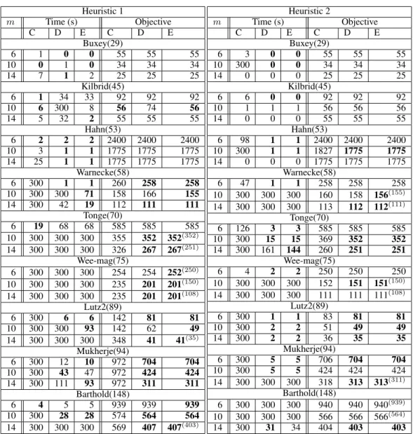
Heuristic 1 m Time (s) Objective C D E C D E Buxey(29) 6 1 0 0 55 55 55 10 0 1 0 34 34 34 14 7 1 2 25 25 25 Kilbrid(45) 6 1 34 33 92 92 92 10 6 300 8 56 74 56 14 5 32 2 55 55 55 Hahn(53) 6 2 2 2 2400 2400 2400 10 3 1 1 1775 1775 1775 14 25 1 1 1775 1775 1775 Warnecke(58) 6 300 1 1 260 258 258 10 300 300 71 158 166 155 14 300 42 19 112 111 111 Tonge(70) 6 19 68 68 585 585 585 10 300 300 300 355 352 352(352) 14 300 300 300 326 267 267(251) Wee-mag(75) 6 300 300 300 254 254 252(250) 10 300 300 300 235 201 201(150) 14 300 300 300 235 201 201(108) Lutz2(89) 6 300 6 6 142 81 81 10 300 300 93 142 62 49 14 300 300 300 348 41 41(35) Mukherje(94) 6 300 12 10 972 704 704 10 300 43 47 972 424 424 14 300 111 93 972 311 311 Barthold(148) 6 4 5 5 939 939 939 10 300 28 28 574 564 564 14 300 300 300 569 407 407(403) Heuristic 2 m Time (s) Objective C D E C D E Buxey(29) 6 3 0 0 55 55 55 10 300 0 0 34 34 34 14 0 0 0 25 25 25 Kilbrid(45) 6 6 0 0 92 92 92 10 1 1 1 56 56 56 14 0 0 0 55 55 55 Hahn(53) 6 98 1 1 2400 2400 2400 10 300 1 1 1827 1775 1775 14 0 0 0 1775 1775 1775 Warnecke(58) 6 47 1 1 258 258 258 10 300 300 300 160 158 156(155) 14 300 300 300 113 112 112(111) Tonge(70) 6 126 3 3 585 585 585 10 300 15 15 369 352 352 14 300 161 144 260 251 251 Wee-mag(75) 6 4 2 2 250 250 250 10 300 300 300 152 151 151(150) 14 300 300 300 111 111 111(108) Lutz2(89) 6 300 1 1 83 81 81 10 300 2 2 51 49 49 14 300 2 2 36 35 35 Mukherje(94) 6 300 5 5 706 704 704 10 300 5 5 424 424 424 14 300 300 300 318 313 313(311) Barthold(148) 6 300 300 300 940 940 940(939) 10 300 300 300 566 566 566(564) 14 300 31 34 404 403 403
Table 2: Results with Heuristics 1 and 2 for settings C, D and E.
given in Table 2. The optimum value is given in exponent between parentheses whenever the optimality could not be proved.
Analysis of results with heuristic 1: The positive effect of the redundant constraints and the global constraint is quite clear. Indeed, settings C, D and E allow to solve and prove the optimality of respectively 11, 17 and 20 instances on a total of 27 within a time limit of 5 minutes (300 seconds). See for example for example Lutz2 instance with 10 work-stations that could be solved only with the global constraint.
Analysis of results with heuristic 2: Settings C, D and E allow to solve and prove the optimality of respectively 10, 20 and 20 instances on a total of 27 within a time limit of 5 minutes (300 seconds). The positive effect of the redun-dant constraints is still impressive but the global constraint
does not allow to solve additional instances. For the instance Warnecke with 10 workstations, the objective is better with the global constraint.
Heuristic 2 allows to solve instances intractable with heuristic 1 (e.g. Barthold 14). The contrary is also true since the Warnecke instance with 10 and 14 workstations cannot be solved with heuristic 2 and can be easily solved with heuristic 1. For the most difficult instances unsolved with both heuristics (Wee-mag 10 and Wee-mag 14), heuristic 2 obtains a better objective value (151<201 and 111<201) very close to the optimal values 150 and 108.
Comparison with state of the art dedicated algorithm:
The state of the art algorithm for this problem is Salome 2 (Klein & Scholl 1996; Scholl & Becker 2006). A binary file of the implementation of the algorithm is available on www.assembly-line-balancing.de. Salome 2 finds the
opti-mal solutions of almost all the instances within less than one second. As with our solution, it is not able to find and prove the optimum for the instances Wee-mag 10 and Wee-mag 14. Salome 2 uses a lot of dominance and reduction rules specific to this problem and objective function.
Generalized Assembly Line Balancing Problem:
SALBP-2 is an academic problem. In real life assembly line problems, additional requirements are possible and the dominance rules used in Salome 2 are not valid anymore. Some possible additional constraints are (Becker & Scholl 2006):
• some tasks must be assigned in the same station, • some tasks can not be assigned in the same station, • there is a restriction on the cumulated value of particular
task attributes,
• some tasks need to be assigned to particular stations, • some tasks can not be assigned to particular stations, • some tasks need a special station,
• some tasks need a minimum distance to other tasks, • some tasks need a maximum distance to other tasks. All these additional constraints can be added very easily in our CP model without changing anything else while ded-icated algorithms such as Salome 2 cannot. To show the flexibility of our approach we have added some constraints to the Barthold instance with 10 workstations to form a Generalized Assembly Line Balancing Problem (GALBP): |B138−B16| ≤ 2,|B104−B41| ≥ 2,|B12−B35| ≤ 2, |B65−B76| ≤ 2,|B101−B102| ≥ 2,|B83−B113| ≥ 2, |B19−B28| ≥3andB16= 4.
The time needed to reach and prove optimality (662) for settings C, D and E with Heuristic 1 are respectively 458, 171 and 143 seconds. Heuristic 2 gives bad results on the GALBP because we designed it specifically for problems with precedence constraints only. Here again, the new re-dundant and global constraints really help to solve the prob-lem faster. This probprob-lem is unsolvable with state of the art dedicated algorithms such as Salome 2.
Another advantage of the constraint programming ap-proach is that the objective function can be easily changed. For example, it is often desirable to smooth the workload among a given number of stations (Becker & Scholl 2006; Scholl & Becker 2006; Rekiek et al. 1999). This prob-lem is called Vertical Line Balancing. This can be effi-ciently achieved in CP with the global constraintsspread anddeviationfor the variance (Pesant & Regin 2005; Schauset al.2006) and the mean absolute deviation (Schaus et al.2007).
Conclusion and Perspectives
We proposed a CP model for BPPC and SALBP-2, al-lowing a flexible expression of new constraints, such as in GALBP. We also designed a global BPPC constraint based on set variables representing the predecessors of each items, which exploits the transitive closure of the precedence
graph. We have conducted an experimental validation on standard SALBP-2 benchmarks, showing the feasibility, the efficiency, and the flexibility of this approach. As future work, we plan to make an hybridization of CP and Local Search through Large Neighborhood Search. We also plan to usespreadanddeviationto solve the Vertical Line Balancing Problem. Currently there exists no exact method for this problem.
Acknowledgements
This research is supported by the Walloon Region, project Transmaze (516207) and partially by Interuniversity Attrac-tion Poles Programme (Belgian State, Belgian Science Pol-icy).
References
Becker, C., and Scholl, A. 2006. A survey on problems and meth-ods in generalized assembly line balancing.European Journal of Operational Research168(3):694–715.
Boysen, N.; Fliedner, M.; and Scholl, A. 2007. A classification of assembly line balancing problems.European Journal of Oper-ational Research674–693.
Castro, C., and Manzano, S. 2001. Variable and value ordering when solving balanced academic curriculum problem. Proc. of the ERCIM WG on constraints.
Cormen, T. H.; Stein, C.; Rivest, R. L.; and Leiserson, C. E. 2001.
Introduction to Algorithms. McGraw-Hill Higher Education. Gervet, C. 1993. New structures of symbolic constraint objects: sets and graphs.
Hnich, B.; Kiziltan, Z.; and Walsh, T. 2002. Modelling a balanced academic curriculum problem.Proceedings of CP-AI-OR-2002. ILOG-S.A. Ilog solver 6.3. user manual.
Klein, R., and Scholl, A. 1996. Maximizing the production rate in simple assembly line balancing: A branch and bound procedure.
European Journal of Operational Research91(2):367–385. Pesant, G., and Regin, J.-C. 2005. Spread: A balancing constraint based on statistics.Lecture Notes in Computer Science3709:460– 474.
Rekiek, B.; De Lit, P.; Pellichero, F.; Falkenauer, E.; and Delchambre, A. 1999. Applying the equal piles problem to bal-ance assembly lines.Proceedings of the 1999 IEEE International Symposium on Assembly and Task Planning399–404.
Schaus, P.; Deville, Y.; Dupont, P.; and R´egin, J. 2006. Simpli-cation and extension of the spread constraint.Third International Workshop on Constraint Propagation And Implementation. Schaus, P.; Deville, Y.; Dupont, P.; and R´egin, J. 2007. The deviation constraint.LNCS CP-AI-OR4510:269–284.
Scholl, A., and Becker, C. 2006. State-of-the-art exact and heuris-tic solution procedures for simple assembly line balancing. Euro-pean Journal of Operational Research168(3):666–693. Scholl, A. 93. Data of assembly line balancing problems. Tech-nische Universitt Darmstadt.
Shaw, P. 2004. A constraint for bin packing. In Wallace, M., ed.,
CP, volume 3258 ofLNCS, 648–662. Springer.
Van Hentenryck P., C. J.-P. 1988. Generality versus specificity: an experience with ai and or techniques.In Proceedings of AAAI-88. van Hoeve, W.-J., and Katriel, I. 2006. Global constraints. In Rossi, F.; Beek, P. V.; and Walsh, T., eds.,Handbook of constraint programming. Elsevier. chapter 6, 169–208.