Using simulation to analyze picker blocking in manual order picking systems

(1)

Peer-review under responsibility of the scientific committee of the 27th International Conference on Flexible Automation and Intelligent Manufacturing doi: 10.1016/j.promfg.2017.07.317

Procedia Manufacturing 11 ( 2017 ) 1798 – 1808

ScienceDirect

27th International Conference on Flexible Automation and Intelligent Manufacturing,

FAIM2017, 27-30 June 2017, Modena, Italy

Using simulation to analyze picker blocking in manual order

picking systems

Behnam Bahrami

a

*

, El-Houssaine Aghezzaf

a

Veronique Limere

b

a_{Department of Industrial Systems Engineering and Product Design,} b_{Department of Business Informatics and Operations Management,} Faculty of Engineering and Architecture, Ghent University, Gent, Belgium

Abstract

The rise of the e-commerce practice makes the warehouses be confronted with ever smaller orders that must be met ever faster, often within a 24-h period. This pressures the order picking process as the orders pickers’ workload becomes higher and higher, leading subsequently to congestion in the warehouse and impacting its productivity. It is therefore crucial to determine which order batching and picking policies enhance the performance of order picking activities. This paper carries out an intensive simulation study to examine the performance of different order picking policies with batching in a wide-aisle warehouse with a low-level picker-to-parts system. The performance of the system is measured in terms of total travelled distance, number of collisions between operators (congestion) and order lead times. A full factorial design is set up and the simulation output is statistically analyzed. The results are reported and thoroughly discussed.

Peer-review under responsibility of the scientific committee of the 27th International Conference on Flexible Automation and Intelligent Manufacturing.

Keywords:Order picking; Batching; Congestion; Simulation

* Corresponding author.

E-mail address: [email protected]

Peer-review under responsibility of the scientific committee of the 27th International Conference on Flexible Automation and Intelligent Manufacturing

(2)

1. Introduction

Warehouses handle inbound functions such as receiving and preparing products for storage, transferring incoming products to storage locations, picking customer’s orders from relevant locations, packing orders on the right unit load (e.g. a carton) and sending demands to destinations (De Koster et al. 2007). Across the various functions in a warehouse, order picking, referred to as the operation of retrieving the required stock keeping units (SKUs) from storage locations to fulfill customer orders, represents over 50% of the total operating cost in a common warehouse (Chiang et al. 2011; Frazelle 2001; Tompkins et al. 2010).

The nowadays fast growing e-commerce practice brings about new challenges for order picking activities. On the one hand, orders have to be met ever faster, often within a 24-h period. On the other hand, individual orders become smaller and smaller. An enormous number of low volume items have to be shipped more frequently and more quickly to clients (Gagliardi et al. 2008). Consequently, more pickers are involved in the picking process taking down order picking performance due to picker blockings (Hong 2015). De Koster and Yu (2006) state that congestion in distribution centers results in less worker productivity, more work stress and higher labor turnover. Moreover, the order fulfillment time can lengthen and operational costs increase.

The aim of this paper is to test and analyze the effect of different routing methods as well as order sequencing and storage strategies executed under different batching methods on low-level picker-to-parts picking performance. In particular, this paper adopts the order-batching methods developed by Ho and Tseng (2006) and carries out intensive simulations of these order-batching methods to evaluate the performance of warehouse picking operations, in terms of number of total distance travelled by operators, collisions between multiple pickers and order lead times (affected by congestion). The effects of different routing methods as well as order sequencing and storage strategies performing under these batching methods are also considered. Among different order picking systems, the most common is the low-level picker-to-parts system in which operators walk or drive (on a proper vehicle) along the aisle to pick items at multiple stops. De Koster et al. (2007) states that over 80% of all Western Europe warehouses implement low-level picker-to-parts picking systems. Therefore, this kind of system is the focus of this study.

The remainder of the paper is organized as follows. Section 2 provides a literature review on order picking operations and a motivation for carrying out these simulations. In Section 3, the problem environment and assumptions are described. Section 4 describes the experimental setup performed to evaluate different warehouse strategies taking picker congestion into account. It also summarizes the analyzed experimental results. Section 5 presents some conclusions and recommendations for further research.

2. Literature review and motivation

The existing research on order picking is quite extensive and various topics have been addressed by different authors. The published contributions in this area focus mainly on the following issues impacting the performance of the order picking system: layout of the warehouse, storage strategy, routing and sequencing policy and order batching. The layout of a warehouse is among the important factors influencing the performance of the order picking system. A study by Caron et al. (2000) has shown that the layout of a warehouse can have an impact of more than 60% on the total travelled distance. Moreover, determining the proper locations of items in the warehouse, i.e. storage assignment, is also a well-researched topic by, among others, (Ene and Öztürk 2012; Li et al. 2015; Manzini et al. 2015; Fontana and Nepomuceno 2016). The effect of order sequencing and routing on order picking performance is also widely studied in the literature (Chen et al. 2014; Kulak et al. 2012; Roodbergen and de Koster 2001). The simulations carried out in this paper provide some results on these effects.

Order batching, which has proven to have a significant impact on order picking (Ruben and Jacobs 1999), is the process of grouping customer orders together and picking them in the same tour. In such methods, orders are grouped into batches. Orders are assigned to a specific batch until the capacity of the batch is exhausted. A variety of approaches have been used to compose order batches. These approaches are based on (i) exact, (ii) heuristic, and (iii) metaheuristic methods (Henn et al. 2012).

This paper adopts the second method of order batching based on heuristic seed algorithms. Seed algorithms were introduced by Elsayed (1981) and generate batches sequentially. These algorithms consist of two distinct steps: seed order selection and order addition. In a first phase, one customer order is selected as an initial order (seed) for a batch which has just been opened. Afterwards, in the order addition phase, customer orders which are “similar” to

(3)

the seed, are added to the batch while taking the capacity of the picking device into account. One of the most comprehensive seed algorithm was proposed by Ho and Tseng, (Ho and Tseng 2006) where the authors consider 9 rules to determine the seed order and 10 criteria to allocate orders to batches. Section 3.1 provides a brief review of this approach.

Until recently, most of the previous studies in picker-to-parts warehousing systems considered only single-picker operations. However, it is a very common situation that multiple order pickers work concurrently within the same picking area. Worker interaction in the same space may sometimes lead to congestion, which reduces worker’s productivity, and in turn increases labor costs (Gue et al. 2006). There are several contributions in literature related to picker blocking and congestion occurring in a warehouse (Gue et al. 2006; Pan et al. 2012; Hong et al. 2012a; Hong et al. 2012b). However, those researchers who have considered congestion in their work, mostly have presented mathematical models. The difficulty of using mathematical models in this field, however, stems from the nature of congestion which is a dynamic feature and hard to capture.

In this paper, we analyze congestion using simulation to get better insight. With simulation many alternative solutions can be tested quickly and easily, with little risk and no disruption to existing processes (Banks et al. 2010). Thus, simulation provides a tool to quantify the impact of congestion, while the various congestion factors and operating conditions change over time. This paper carries out intensive simulations of several heuristic batching methods described in Ho and Tseng (2006). It combines various storing, sorting and routing policies to compare and analyze the performance of a low-level picker-to-part order picking system. It focuses in particular on the congestion resulting from multiple pickers in a warehouse. The measures of performance that considered in this investigation are total distance travelled by order pickers, number of collisions between pickers and order lead times. The latter being influenced by congestion.

3. Problem environment and description

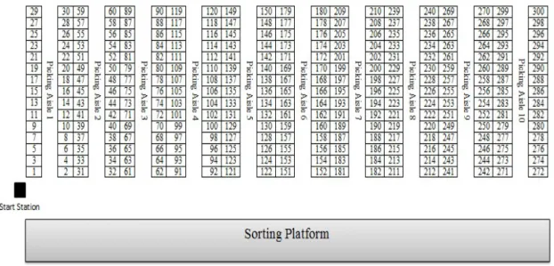
The warehouse investigated in this paper is a low-level picker-to-parts manual order picking system, as presented in Fig. 1. The layout structure is composed of 10 parallel wide aisles which are indexed from 1 to 10, and each aisle has 30 picking locations. Operators are able to move within an aisle in both directions and are allowed to change their direction within an aisle. The aisles are wide enough such that operators can cross each other. At the front and back of the aisles there are cross aisles to switch from one pick aisle to another pick aisle. The start station is located at the bottom left corner of the first aisle. Order pickers begin at the start station where they collect pick lists as well as carts. Then, they walk through the picking area and retrieve items from different slots. After finishing all picks, they go to the sorting platform where the items are left for shipping (sort-after-pick). The warehouse uses a wave picking policy, i.e. when a large set of customer orders is assigned to a pre-defined shipping schedule (called wave), all requested items must be picked and shipped within the corresponding wave. Each wave typically is a combination of a number of batches which are picked simultaneously by a group of order pickers (Gademann et al. 2001). Every order picker picks one batch and all order pickers start at the same time. In this paper, it is assumed that at the beginning of a wave, the set of orders that needs to be picked in the wave (order pool) is already known, and the orders are randomly generated. The distribution of the set of orders in the wave is done according to the type of storage policy, which will be explained later in more details. Before a wave begins, the set of orders in the order pool are grouped in batches, based on one of the batching methods proposed by (Ho and Tseng 2006) briefly reviewed in section 3.1. Then, each batch is assigned to one order picker who is ready to start his trip at the start station. It is assumed here that the size of each batch, defined as the number of items, is not greater than the picking cart’s capacity, which is 100 items. Another assumption is that one order is not split into different batches to avoid additional sorting efforts and the time needed to wait until an order is completed by a number of operators. The wave is started when all batches are assigned to order pickers. At this point, pickers receive their pick lists (a pick list is a batch) which describe the storage locations that are to be visited and the corresponding number of items requested for each sku. The picking routes are determined by one of the routing methods considered, as explained in the next subsection. As mentioned, this paper addresses a warehouse with multiple pickers working concurrently in the same area, generating inevitably congestion. In the studied warehouse, congestion can occur in three ways: (i) when two or more pickers reach to the same picking face and attempt to occupy the same space simultaneously ; (ii) when a picker enters an aisle to retrieve items while the aisle is occupied by other pickers in a way that they cannot pass each other (iii) when blocking occurs in cross aisles.

(4)

Figure 1. Warehouse layout

3.1 Batching Methods

For this study we adopt the order batching methods described in Ho and Tseng (2006). The authors implemented a seed algorithm to generate batches. They introduced 9 seed-order (SO) selection rules and 10 accompanying-order (AO) selection rules, summarized in following tables, to make a batch and assign it to a picker. The order-batching process to form an order batch works as follows: a seed order S is selected first from the order pool P using one of seed-order selection rules. The selected seed order is the first order added to the order batch B. Then the remaining capacity of the batch, RC, is updated by subtracting the capacity demand of the seed from the picking cart’s capacity. After that, among all remaining orders with a capacity demand smaller than or equal to RC (set QS), an order is chosen based on an accompanying-order selection rule and is added to the order batch. Next, the remaining capacity of the picking cart is updated again, and the accompanying-order selection process is repeated until the picking cart is full and cannot accept any more orders. At this point, the first batch has been prepared and is assigned to the first picker. The same procedure is repeated for the next batch and next picker until all orders are batched.

Table 1. Summary of seed order (SO) selection rules. (see Ho and Tseng, 2006, for more details)

Seed-order selection rules Definition

Random(RD) The SO is randomly selected from the order pool.

Smallest No_{of Picking Locations (SNPL)} _{The order which has the smallest number of picking locations to visit is selected as the SO.} Greatest No_{of Picking Locations (GNPL)} _{The order which has the greatest number of picking locations to visit is selected as the SO.} Smallest No_{of Picking Aisles (SNPA)} _{The order that has the smallest number of picking aisles to visit is selected as the SO.} Greatest No_{of Picking Aisles (GNPA)} _{The order that has the greatest number of picking aisles to visit is selected as the SO.} Smallest Location-Aisle Ratio (SLAR) For every order in the order pool, LAR ( Location-Aisle Ratio) is:

where NofPL (R) = the number of picking locations of order R; NofPA (R) = the number of picking aisles of order R. The order with the smallest LAR is selected as the SO. Greatest Location-Aisle Ratio (GLAR) Opposite to the SLAR rule, one selects the order with the greatest LAR as the SO. Smallest Aisle-Weight Sum (SAWS)

For every order in the order pool, AWS (Aisle-Weight Sum) is:

where i = aisle index; AS(R) = the set of aisles that contain the items of order R; =

(the farther away from the I/O, the greater an aisle’s weight AWi) The order with the smallest AWS is selected as the SO.

(5)

Table2. Summary of accompanying rules(AO). (see Ho and Tseng, 2006, for more details)

3.2 Routing policy

The objective of routing policies is to sequence the items on the pick list to ensure a good route through the warehouse. Two order picking policies are considered in this study:

S-shape routing: This means that any aisle containing at least one pick is traversed entirely (except potentially the last visited aisle). Aisles without picks are not entered. From the last visited aisle, the order picker returns to the sorting platform.

Return method: With this method an order picker enters and leaves each aisle from the same end. Only aisles with picks are visited.

3.3 Sorting methods

Sorting methods describe how the items in an order are sorted and the sequence of locations visited by an order picker. The three considered methods in this study are:

No sorting: The items are not sorted. As a consequence, the order picker may visit the same aisle multiple times. Random aisle: The list of items is only sorted based on aisle. Items within the same aisle are grouped together and sorted such that the item closest to the order picker is picked first. The order picker can visit each aisle at most once. However, the sequence in which the aisles are visited is not sorted.

Completely sorted: The items are sorted by aisle as described above, and, moreover, the sequence of the aisles visited is sorted from left to right. Aisles with no items to pick are skipped.

Accompanying-order selection rules Definition

Random(RD) The AO is randomly selected from the order pool.

Smallest No_{of Additional Picking Locations} (SNAPL)

The order with smallest number of additional picking locations, if order R is added to batch B, is selected as the AO.

Smallest No_{of Additional Picking Aisles} (SNAPA)

The order with the smallest number of additional picking aisles, if order R is added to batch B, is selected as the AO.

Greatest No_{of Identical Picking Locations} (GNIPL)

The order with the highest similarity to the batch, in terms of picking locations, is selected as the AO.

Greatest No_{of Identical Picking Aisles} (GNIPA)

The order with the highest similarity to the batch, in terms of picking aisles, is selected as the AO.

Greatest Picking-Location Similarity Ratio (GPLSR)

The order with the greatest PLSR, is selected as the AO:

where NIPL(R,B) = number of identical picking locations between order R and the orders in B; TNofPL(R, B) = total number of picking locations that the picker needs to visit if R is added to B.

Greatest Picking-Aisle Similarity Ratio (GPASR)

The order with the greatest PASR, is selected as the AO:

where NIPA(R, B) = number of identical picking aisles between R and the orders in B; TNofPA(R, B) = total number of picking aisles that the picker needs to visit if R is added to B. Greatest Picking-Location Covering Ratio

(GPLCR)

The order with the greatest PLCR, is selected as the AO:

where NIPL(R,B) = number of identical picking locations between R and the orders in B; NofPL(R) = number of picking locations of order R.

Greatest Picking-Aisle Covering Ratio (GPACR)

The order with the greatest PACR, is selected as the AO:

where NIPA(R, B) = number of identical picking aisles between R and the orders in B; NofPA(R, B) = number of picking aisles of order R.

Greatest Identical-Location to Additional-Aisle Ratio (GILAAR)

The order with the greatest ILAAR, is selected as the AO:

where NIPL(R,B) = number of identical picking locations between R and the orders in B; NAPA(R, B) = number of additional picking aisles that the picker needs to visit if R is added to B.

(6)

3.4 Storage assignments

To evaluate whether the assignment of storage space has any influence on the performance of the system, two sets of orders are generated according to two types of storage policies. In the first set, it is assumed that the locations of the items are random and orders are randomly distributed throughout the entire warehouse. This means that every aisle has the same chance to be visited. However, in the second set we assume that popular items are placed in the aisles closest to the start station. The top 50% of the most popular items are randomly distributed in aisles 1, 2 and 3; aisles 4, 5, 6 and 7 store the next 30 % of items; and the remaining items are randomly distributed in aisles 8, 9 and 10. This is called class-based storage.

4. Simulation and results analysis

4.1 The simulation model

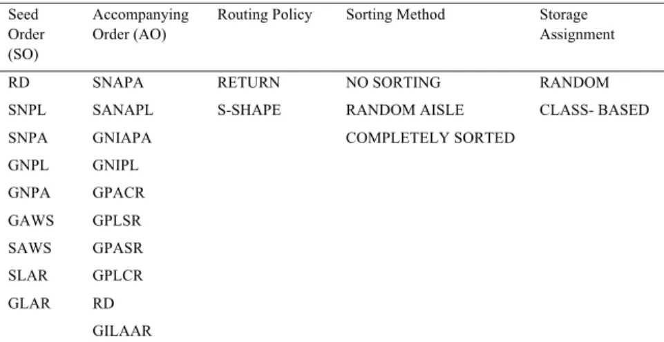
All experiments are simulated with Flexsim 7.5 software. The objective of the simulation is to capture the effect of the different batching, routing, storage policies and sorting methods on congestion. Aside from the number of collisions, the total travelled distance and the order lead times are also studied. The layout of the warehouse considered in the simulation is shown in Fig. 1. The width of every aisle within the warehouse is 2 meters. The speed of the operators is assumed to be 1 m per second. Each operator can operate one cart which has a capacity of 100 units. To provide a better basis for analyzing the system, 10 Order pools have been generated randomly in this study. Each order pool contains 75 orders and the number of different items in an order is uniformly generated from 1 to 20. In addition the quantity of each requested item varies from 1 to 4. Finally, it is assumed that there are enough operators to pick all requested items. Table 3 summarizes the full factorial design of experiments.

Table 3. Factors considered in the experiment Seed

Order (SO)

Accompanying Order (AO)

Routing Policy Sorting Method Storage Assignment RD SNPL SNPA GNPL GNPA GAWS SAWS SLAR GLAR SNAPA SANAPL GNIAPA GNIPL GPACR GPLSR GPASR GPLCR RD GILAAR RETURN S-SHAPE NO SORTING RANDOM AISLE COMPLETELY SORTED RANDOM CLASS- BASED

In total (9*10*2*3*2) = 1080 combinations of factors must be examined. Since each combination is replicated 10 times, a total of 10800 simulations were carried out.

4.2 Analysis of the results

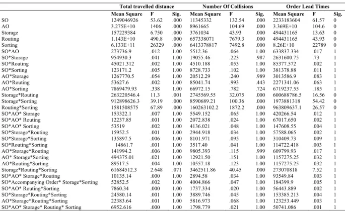
The results are analyzed by ANOVA and presented in the following tables.

The results in table 4 indicate that, for the three performance measures, total travelled distance, number of collisions, and order lead time, all of the main factors are significant at an α of 0.05. In addition, for travel distance, three of the ten two-way interactions and one of the three-way interactions are significant at an α of 0.05. In terms of collisions, four two-way interactions and one of the three- way interactions are significant at an α of 0.05. For order lead time, three of two-way interactions and one of the three-way interactions are significant at level of 0.05. Tables 4 , 5 and 6 present the mean for all three measures of performance and the 95% confidence interval for order-picking routing,

(7)

storage assignment and sorting rules respectively. Table 4. Full factorial ANOVA

Total travelled distance Number Of Collisions Order Lead Times

Mean Square F Sig. Mean Square F Sig. Mean Square F Sig.

SO 1249046926 53.62 .000 11345332 132.54 .000 2233183604 61.57 0

AO 3.275E+10 1406 .000 8961665 104.69 .000 3.369E+10 104.6 0

Storage 157229384 6.750 .000 3761034 43.93 .000 494431165 13.63 0

Routing 1.143E+10 490.8 .000 657338071 7679.3 .000 494431165 43.93 0

Sorting 6.133E+11 26329 .000 6413378817 7492.8 .000 8.26E+10 22789 0

SO*AO 273736.9 .012 1.00 5512.36 .064 1.00 633837.334 .017 1 SO*Storage 954930.3 .041 1.00 19055.46 .223 .987 2631600.75 .73 1 SO*Routing 45021.312 .002 1.00 4510.188 .053 1.00 85377.572 .002 1 SO*Sorting 123171.2 .005 1.00 8728.733 .102 1.00 381378.88 .011 1 AO*Storage 1267770.5 .054 1.00 20512.29 .240 .989 3013586.9 .083 1 AO*Routing 53627.6 .002 1.00 85041.74 .993 .443 2271341.06 .063 1 AO*Sorting 7869479.93 .338 1.00 66972.15 .782 .724 6719237.55 .185 1 Storage*Routing 263220546.4 11.3 .001 2745569.55 32.075 .000 600688786.5 16.56 0 Storage*Sorting 912898626.3 39.19 .000 8590689.21 100.36 .000 1973881318 54.42 0 Routing*Sorting 1581508575 67.89 .000 160263102.2 1872.2 .000 963809637.1 26.57 0 SO*AO* Storage 153322.1 .007 1.00 5549.152 .065 1.00 420266.54 .012 1 SO*AO* Routing 12237.85 .001 1.00 2072.838 .024 1.00 67017.650 .002 1 SO*AO* Sorting 53519 .002 1.00 4136.021 .048 1.00 147608.55 .004 1 SO*Storage*Routing 15952.5 .001 1.00 2944.918 .034 1.00 57588.065 .002 1 SO*Storage*Sorting 135897.5 .006 1.00 8101.971 .095 1.00 310409.73 .009 1 SO*Routing*Sorting 14861.7 .001 1.00 3517.40 .041 1.00 114722.418 .003 1 AO*Storage*Routing 141994.2 .006 1.00 9805.393 .115 .999 609799.93 .017 1 AO* Storage*Sorting 494375.01 .021 1.00 12921.50 .151 1.00 1157275.25 .032 1 AO*Routing*Sorting 89517.5 .004 1.00 10557.18 .123 1.00 1157275.25 .032 1 Storage*Routing*Sorting 61684512.3 2.648 .071 3462511.86 40.45 .000 273070818 7.52 1 SO*AO* Storage*Routing 10135.14 .000 1.00 2894.58 .034 1.00 93549.84 .003 1

SO*Accompanying Order* Storage*Sorting 52852.5 .002 1.00 4004.866 .047 1.00 184399.9 .005 1

SO*AO* Routing*Sorting 7860.34 .000 1.00 1737.334 .020 1.00 56443.889 .002 1

SO*Storage*Routing*Sorting 24580.14 .001 1.00 3889.746 .045 1.00 153385.213 .004 1

AO*Storage*Routing*Sorting 22383.64 .001 1.00 5816.973 .068 1.00 123253.449 .003 1 SO*AO* Storage* Routing* Sorting 6952.616 .000 1.00 1798.779 .021 1.00 50741.086 .001 1

Table 5. Performance factor means and 95% confidence intervals of Return and S-shape.

Dependent Variable Routing Mean Std. Error Upper Bound Lower Bound Total travelled distance RETURN 25348.874 65.676 24786.541 26908.613

S-SHAPE _26256.368 _65.676 _26102.005 _26966.449

Number Of Collisions RETURN 1294.397 3.981 1286.593 1302.201

S-SHAPE 800.982 3.981 793.177 808.786

Order Lead Time RETURN 32896.859 81.956 32736.209 33057.509

S-SHAPE _30487.619 _81.956 _30326.969 _30648.269 Table 6.Performance factor means and 95% confidence intervals of CLASS-BASED and RANDOM.

Dependent Variable Distribution Mean Std. Error Lower Bound Upper Bound Total travelled distance CLASS-BASED 26358.711 65.676 26185.500 27058.189

RANDOM 26716.520 65.676 26559.395 26816.873

Number Of Collisions CLASS-BASED 1066.351 3.981 1058.546 1074.155

RANDOM 1029.028 3.981 1021.224 1036.833

Order Lead Time CLASS-BASED 31906.203 81.956 31745.553 32066.853

(8)

Table 7. Performance factor means and 95% confidence intervals of Sorting methods.

Dependent Variable Sorting Mean Std. Error Lower Bound Upper Bound

Total travelled distance NO SORTING 42056.621 80.437 41671.913 42369.784

COMPLETE SORTING 18197.548 80.437 18073.723 18389.069

RANDOMLY SORTED 20450.698 80.437 20207.720 20598.145

Number Of Collisions NO SORTING 1534.957 4.876 1525.399 1544.516

RANDOMLY SORTED 794.666 4.876 785.107 804.224

Order Lead Time NO SORTING 49149.373 100.375 48952.618 49346.128

RANDOMLY SORTED 23983.722 100.375 23786.967 24180.478

Table 8. Performance factor means and 95% confidence intervals of Seed order selection rules. Dependent Variable Seed Order Mean Std. Error Lower Bound Upper Bound Total travelled distance GAWS 28865.23 139.321 28317.853 28970.577

GLAR 26765.25 139.321 26460.299 27006.493 GNPA 27931.66 139.321 27409.379 27955.574 GNPL 28118.33 139.321 27435.426 28467.714 RD 26655.10 139.321 26271.063 26817.257 SAWS 26384.92 139.321 25805.340 26445.017 SLAR 26802.54 139.321 26486.253 27032.448 SNPA 25844.56 139.321 25314.314 25860.509 SNPL 25911.72 139.321 25321.321 25945.100 Number Of Collisions GAWS 1104.036 8.446 1087.480 1120.591

GLAR 1101.700 8.446 1085.144 1118.256 GNPA 1099.092 8.446 1082.537 1115.648 GNPL 1107.758 8.446 1091.202 1124.313 RD 1210.036 8.446 1193.480 1226.591 SAWS 950.909 8.446 934.354 967.465 SLAR 956.941 8.446 940.385 973.496 SNPA 949.028 8.446 932.473 965.584 SNPL 949.705 8.446 933.149 966.261 Order Lead Time GAWS 33756.12 173.854 33415.339 34096.920

GLAR 31886.89 173.854 31546.106 32227.686 GNPA 32822.93 173.854 32482.149 33163.729 GNPL 32892.31 173.854 32551.521 33233.101 RD 32239.33 173.854 31898.549 32580.129 SAWS 30477.98 173.854 30137.193 30818.774 SLAR 31189.05 173.854 30848.265 31529.845 SNPA 29977.55 173.854 29636.763 30318.343 SNPL 29987.94 173.854 29647.153 30328.734

From obtained results, it can be concluded that the RETURN method is considerably better than the S-SHAPE method in terms of travelled distance. However, for collisions and lead time, S-SHAPE routing outperforms the RETURN method. The reason is that in RETURN routing, order pickers collide when they return through the same

(9)

aisle, which results in delays, increasing the order lead times. From the table 6, one can conclude that the class based policy outperforms the random policy in total travelled distance. This was expected since top ranked items are placed in aisles close to the start station. On the other hand, implementing a class-based policy when more operators work in the same area, will increase the number of collisions within the warehouse as well as the order lead times.

Regarding the different sorting rules, of which factors’ performance means and confidence intervals are indicated in table 7, it can be concluded that COMPLETE SORTING has the best performance in terms of travelled distance, followed by RANDOM and NO SORTING rule. Table 7 also reveals that if the NO SORTING rule is selected as sorting method, there will be a considerable rise in order lead times and collisions.

Based on the results of table 8, SNPA is the best method while GAWS is the worst one.it also can be seen that, among all nine seed rules, SNPA, SNPL, and SAWS have a better performance in total travelled distance. This means they are not significantly different (at an α of 0.05) in their performance, but they are all significantly better than the other seed-order selection rules at an α of 0.05. On the other hand, GNPA, GNPL and GAWS are the three worst rules. According to the analyzed results from tables 8, it can be noticed that SNPA, SNPL, SAWS and SLAR perform well in terms of both number of collisions and orders lead time, while GNPL, GAWS AND RANDOM perform poorly. Additionally, it can be concluded that the smallest value-based rules (i.e. SNPL, SNPA, SAWS, and SLAR) are all better than greatest value-based rules (i.e. GLAR, GNPL, GNPA, and GAWS). In addition, the RD rule is worse than the all greatest-value-based rules in collisions and order lead time. Table 9 presents the factors performance means of each accompanying order selection for total travelled distance, number of collisions and orders lead time respectively. From this table, one can notice that SNAPA has the best performance on total travelled distance and the RANDOM rule has the worse results. Table 9 also shows that all accompanying order rules are better than RANDOM rules in distance based performance. In addition, the top four rules (i.e. SNAPA, GNIPA, GPACR, and GILAAR) are all related to aisle-based values.

5. Conclusion

The aim of this investigation is to study and analyze the performance of a low-level order picking warehouse when multiple operators work simultaneously. In our analysis, a wide range of designs were explored. The designs that we considered include the seed order batching method outlined in (Ho and Tseng 2006), three types of sorting methods, storage assignment rules and two routing policies. The experiments were carried out to measure warehouse performance in terms of total distance travelled by pickers, number of collisions among pickers and resulting order lead time including congestion effects. Simulation models were hired to determine the impact that various operating strategies may have on the warehouse and determine which ones are the best to pursue. In total 10800 simulation models were implemented and the results were analyzed via full factorial ANOVA. The results show that congestion has a direct impact on order lead time. Additionally, the experimental analyses discussed in this paper also provided the following conclusions.

The results also indicate that the best configuration for the total travelled distance is obtained using a return routing policy and class-based storage strategy while orders in picking lists are sorted in a way that all aisles and location within aisles are sequenced( in the studied case from left to right).Regarding the seed selection rules, the smallest value-based rules (i.e. SNPL, SNPA, SAWS, and SLAR) perform better than greatest value-based rules (i.e. GLAR, GNPL, GNPA, and GAWS) while, the RD rule performs poorly that than all other rules for collisions and order lead time and outperforms greatest value-based rules in terms of total distance travelled. Concerning the accompanying rules, the best rule is Smallest Number of Additional Picking Aisles (SNAPA).

(10)

References

[1] Caron F, Marchet G, Perego A (2000) Optimal layout in low-level picker-to-part systems International Journal of Production Research 38:101-117

[2] Chiang DM-H, Lin C-P, Chen M-C (2011) The adaptive approach for storage assignment by mining data of warehouse management system for distribution centres Enterprise Information Systems 5:219-234 doi:10.1080/17517575.2010.537784

[3] Chen F, Wang H, Xie Y, Qi C (2014) An ACO-based online routing method for multiple order pickers with congestion consideration in warehouse Journal of Intelligent Manufacturing:1-20

[4] De Koster M, Van der Poort ES, Wolters M (1999) Efficient orderbatching methods in warehouses International Journal of Production Research 37:1479-1504

[5] De Koster R, Yu M Makespan minimization at Aalsmeer flower auction. In: 9th International material handling research colloquium, Salt Lake City, Utah, 2006.

[6] Ene S, Öztürk N (2012) Storage location assignment and order picking optimization in the automotive industry The international journal of advanced manufacturing technology 60:787-797

[7] Frazelle E (2001) World-Class Warehousing and Material Handling. McGraw-Hill Education,

Dependent Variable AO Mean Std. Error Lower Bound Upper Bound Total travelled distance GILAAR 23890.654 146.857 23453.129 24028.869 GNIPA 19666.083 146.857 19509.139 20084.879 GNIPL 26100.005 146.857 25531.613 26107.352 GPACR 21726.396 146.857 21468.839 22044.579 GPASR 32501.214 146.857 31711.681 32996.609 GPLCR 32523.168 146.857 31723.881 32603.076 GPLSR 30789.439 146.857 29671.370 31098.651 RD 35790.380 146.857 34856.331 36905.466 SNAPA 19465.654 146.857 19292.442 19868.182 SNAPL 28411.932 146.857 27990.791 28709.543 Number Of Collisions GILAAR 1093.698 8.903 1076.247 1111.149

GNIPA 1153.461 8.903 1136.010 1170.912 GNIPL 1154.128 8.903 1136.677 1171.579 GPACR 1054.614 8.903 1037.163 1072.065 GPASR 1074.194 8.903 1056.743 1091.646 GPLCR 1074.938 8.903 1057.487 1092.389 GPLSR 1072.281 8.903 1054.829 1089.732 RD 1001.337 8.903 983.886 1018.788 SNAPA 870.346 8.903 852.895 887.797 SNAPL 927.897 8.903 910.446 945.348 Order Lead Time GILAAR 28459.490 183.258 28100.265 28818.714

GNIPA 24564.315 183.258 24205.090 24923.539 GNIPL 30590.121 183.258 30230.897 30949.346 GPACR 26579.779 183.258 26220.554 26939.003 GPASR 36920.523 183.258 36561.299 37279.748 GPLCR 36936.440 183.258 36577.216 37295.665 GPLSR 34870.643 183.258 34511.418 35229.867 RD 40150.886 183.258 39791.662 40510.111 SNAPA 24432.044 183.258 24072.819 24791.268 SNAPL 33418.147 183.258 33058.923 33777.372 Table 9. Performance factors means and 95% confidence intervals of each accompanying-order selection rule.

(11)

[8] Gagliardi J-P, Ruiz A, Renaud J (2008) Space allocation and stock replenishment synchronization in a distribution center International Journal of Production Economics 115:19-27

[9] Fontana ME, Nepomuceno VS (2016) Multi-criteria approach for products classification and their storage location assignment The International Journal of Advanced Manufacturing Technology:1-12

[10] Gademann A, Van Den Berg JP, Van Der Hoff HH (2001) An order batching algorithm for wave picking in a parallel-aisle warehouse IIE transactions 33:385-398

[11] Gue KR, Meller RD, Skufca JD (2006) The effects of pick density on order picking areas with narrow aisles IIE transactions 38:859-868 [12] Henn S, Koch S, Wäscher G (2012) Order batching in order picking warehouses: a survey of solution approaches. Springer,

[13] Ho Y-C, Tseng Y-Y (2006) A study on order-batching methods of order-picking in a distribution centre with two cross-aisles International Journal of Production Research 44:3391-3417

[14] Hong S (2015) Order Batch Formations for Less Picker Blocking in a Narrow-Aisle Picking System Industrial Engineering & Management Systems 14:289-298

[15] Hong S, Johnson AL, Peters BA (2012a) Batch picking in narrow-aisle order picking systems with consideration for picker blocking European Journal of Operational Research 221:557-570

[16] Hong S, Johnson AL, Peters BA (2012b) Large-scale order batching in parallel-aisle picking systems IIE Transactions 44:88-106

[17] kulak O, Sahin Y, Taner ME (2012) Joint order batching and picker routing in single and multiple-cross-aisle warehouses using cluster-based tabu search algorithms Flexible services and manufacturing journal 24:52-80

[18] Li J, Moghaddam M, Nof SY (2015) Dynamic storage assignment with product affinity and ABC classification—a case study The International Journal of Advanced Manufacturing Technology:1-16.

[19] Manzini R, Accorsi R, Gamberi M, Penazzi S (2015) Modeling class-based storage assignment over life cycle picking patterns International Journal of Production Economics 170, Part C:790-800

[20] Pan JC-H, Shih P-H, Wu M-H (2012) Storage assignment problem with travel distance and blocking considerations for a picker-to-part order picking system Computers & Industrial Engineering

[21] Roodbergen KJ, Vis IF, Taylor Jr GD (2015) Simultaneous determination of warehouse layout and control policies International Journal of Production Research 53:3306-3326